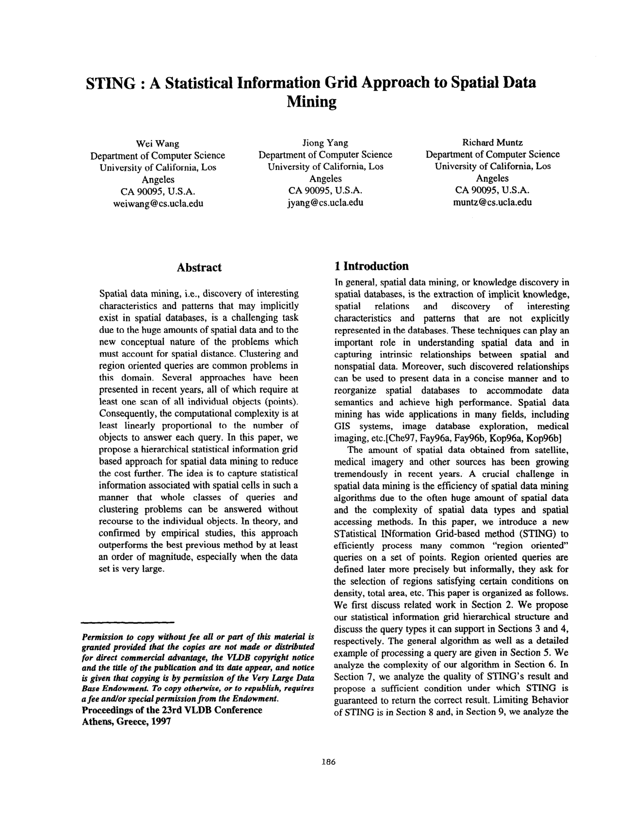
STING: A Statistical Information Grid Approach to Spatial Data Mining

Wei WangJiong YangRichard Muntz

article1997VLDB1,529 citations

Proposes a hierarchical statistical information grid approach called STING that answers spatial clustering and region-oriented queries in time proportional to grid cell count rather than dataset size, speeding up query processing by an order of magnitude on large spatial databases.

Listen

Rapidly expanding volumes of geographic, medical, and satellite data have made spatial data mining increasingly critical for discovering hidden patterns and regional characteristics. Existing spatial clustering and query methods—such as CLARANS, BIRCH, and DBSCAN—suffer from a major computational bottleneck: they are query-dependent and require scanning individual data records at least once per query. As datasets grow into millions of records, this object-dependent scanning results in substantial processing delays and high computational costs.

The article introduces and evaluates STING (Statistical Information Grid), a hierarchical grid-based approach designed to execute region-oriented spatial queries efficiently. The core objective is to demonstrate that precomputing and storing statistical summaries across multi-resolution spatial cells allows systems to answer spatial queries and perform clustering without repeatedly accessing individual data points.

To evaluate this approach, the authors designed a hierarchical framework where space is divided into rectangular cells across multiple layers, capturing parameters such as object counts, attribute means, standard deviations, min-max ranges, and statistical distribution types. Query processing proceeds top-down from higher to lower resolutions, pruning irrelevant regions using statistical confidence intervals. The authors analyzed the computational complexity theoretically, mathematically proved sufficient conditions for spatial query accuracy, and empirically tested performance using benchmark datasets, including the SEQUOIA 2000 storage benchmark and synthetic datasets of 100,000 spatial points.

The key findings demonstrate major performance and scalability advantages. First, query processing in STING depends entirely on the number of leaf grid cells rather than the total number of raw objects. Because the number of grid cells is typically several orders of magnitude smaller than the number of objects, the method achieves massive runtime reductions. Second, in benchmark tests across thousands of data points, STING answered queries in roughly 0.12 to 0.14 seconds, outperforming DBSCAN query execution by at least an order of magnitude and surpassing randomized search methods like CLARANS by hundreds of times. Third, precomputation of the grid hierarchy requires only a single data pass, taking under 10 seconds for 100,000 points, and the structure supports incremental updates when new data arrives without full recomputation. Finally, mathematical analysis confirms that as cell granularity approaches zero, the limiting behavior of STING converges to that of DBSCAN, ensuring high clustering quality.

These findings indicate that adopting a statistical grid architecture substantially reduces server workloads, operational query latency, and data input/output overhead. Because the grid summary is compact enough to remain in memory, organizations handling large-scale spatial analytics can execute frequent interactive queries at minimal infrastructure cost. Furthermore, because individual grid cells can be evaluated independently, the architecture is easily parallelizable for distributed computing environments.

Organizations managing large spatial databases should consider implementing statistical summary grids for interactive, region-oriented analytical workloads. Decision-makers should leverage this architecture when high-throughput exploratory querying is required across stable or incrementally updated spatial datasets. For future technical development, extending the framework to handle non-numerical categorical attributes and evaluating multidimensional spatial models beyond two dimensions represent the most valuable next steps.

The findings are supported with high confidence by mathematical proofs and benchmark experiments, though certain operational limitations apply. Spatial boundaries returned by the grid approximation may exhibit slight variations compared to exact point scans, and highly precise boundary requirements may still require targeted secondary retrieval of raw data from the underlying database. Additionally, current evaluations focus on numerical attributes, meaning confidence is highest for numerical spatial queries.

Cover for STING: A Statistical Information Grid Approach to Spatial Data Mining

Abstract

Spatial data mining, i.e., discovery of interesting characteristics and patterns that may implicitly exist in spatial databases, is a challenging task due to the huge amounts of spatial data and to the new conceptual nature of the problems which must account for spatial distance. Clustering and region oriented queries are common problems in this domain. Several approaches have been presented in recent years, all of which require at least one scan of all individual objects (points). Consequently, the computational complexity is at least linearly proportional to the number of objects to answer each query. In this paper, we propose a hierarchical statistical information grid based approach for spatial data mining to reduce the cost further. The idea is to capture statistical information associated with spatial cells in such a manner that whole classes of queries and clustering problems can be answered without recourse to the individual objects. In theory, and confirmed by empirical studies, this approach outperforms the best previous method by at least an order of magnitude, especially when the data set is very large.

Table of Contents

  • 1 Introduction
  • 2 Related Work
  • 2.1 Generalization-based Approach
  • 2.2 Clustering-based Approach
  • 2.2.1 CLARANS
  • 2.2.2 BIRCH
  • 2.2.3 DBSCAN
  • 3 Grid Cell Hierarchy
  • 3.1 Hierarchical Structure
  • 3.2 Parameter Generation
  • 4 Query Types
  • 5 Algorithm
  • 6 Analysis of the STING Algorithm
  • 7 Quality of STING
  • 8 Limiting Behavior of STING is Equivalent to DBSCAN
  • 9 Performance
  • 9.1 Performance Comparison of Two Distributions
  • 9.2 Benchmark Result
  • 10 Conclusion
  • Acknowledgments
  • References

Knowls

  1. Knowl 1 — STING Hierarchical Grid Structure and Cell Parameter Representation

    model/method

    The Statistical Information Grid (STING) represents a spatial database by partitioning a continuous spatial area hierarchically into rectangular grid cells across multiple resolution layers. At level 1 (the top layer), the root cell encompasses the entire spatial area. A cell at level ii corresponds to the union of the spatial areas of its child cells at level i+1i+1. In the standard two-dimensional setting, each non-leaf cell is partitioned into 4 child quadrants. The size of the leaf-level (bottom layer) cells is chosen such that the average number of spatial objects per leaf cell ranges from several dozens to several thousands.

    Each cell stores statistical summaries of the spatial objects contained within its spatial boundary, separated into attribute-independent and attribute-dependent parameters:

    • Attribute-independent parameter:
      • n∈Nn \in \mathbb{N}: the number of spatial points located within the cell.
    • Attribute-dependent parameters (stored for each numerical attribute):
      • m∈Rm \in \mathbb{R}: the arithmetic mean of the attribute values in the cell.
      • s∈R≥0s \in \mathbb{R}_{\ge 0}: the standard deviation of the attribute values in the cell.
      • min⁡∈R\min \in \mathbb{R}: the minimum value of the attribute in the cell.
      • max⁡∈R\max \in \mathbb{R}: the maximum value of the attribute in the cell.
      • dist∈{NORMAL,UNIFORM,EXPONENTIAL,…,NONE}\text{dist} \in \{\text{NORMAL}, \text{UNIFORM}, \text{EXPONENTIAL}, \dots, \text{NONE}\}: the probability distribution type followed by the attribute in this cell, determined by hypothesis testing (such as a χ2\chi^2-test) or set to NONE\text{NONE} if the distribution is unknown or heterogeneous.

    This grid hierarchy is constructed query-independently in a single pass over the dataset and supports incremental updates when objects are inserted or modified.

  2. Knowl 2 — Bottom-Up Parameter Aggregation in the STING Cell Hierarchy

    equation

    For bottom-layer (leaf) cells in STING, summary statistics are calculated directly from raw data points. For any non-leaf cell at a higher layer, its statistical parameters are recursively computed from the parameters of its constituent lower-level child cells indexed by ii. Let ni,mi,si,min⁡i,max⁡in_i, m_i, s_i, \min_i, \max_i, and disti\text{dist}_i denote the parameters of child cell ii. The aggregated parameters n,m,s,min⁡,max⁡n, m, s, \min, \max for the parent cell are:

    n=∑inin = \sum_i n_i

    m=∑imininm = \frac{\sum_i m_i n_i}{n}

    s=∑i(si2+mi2)nin−m2s = \sqrt{\frac{\sum_i (s_i^2 + m_i^2) n_i}{n} - m^2}

    min⁡=min⁡i(min⁡i)\min = \min_i (\min_i)

    max⁡=max⁡i(max⁡i)\max = \max_i (\max_i)

    The distribution type dist\text{dist} of the parent cell is assigned using a majority-and-conflict rule with a conflict tolerance threshold τ\tau (typically τ=0.05\tau = 0.05):

    1. Candidate dist\text{dist} is initialized to the distribution type associated with the majority of points among all child cells (i.e., maximizing ∑disti=distni\sum_{\text{dist}_i = \text{dist}} n_i).
    2. A conflict point count confl\text{confl} is initialized to 00 and updated across child cells:
      • If disti≠dist\text{dist}_i \ne \text{dist}, but mi≈mm_i \approx m and si≈ss_i \approx s, then confl←confl+ni\text{confl} \leftarrow \text{confl} + n_i.
      • If disti≠dist\text{dist}_i \ne \text{dist}, and either mi≉mm_i \not\approx m or si≉ss_i \not\approx s, then confl←n\text{confl} \leftarrow n.
      • If disti=dist\text{dist}_i = \text{dist}, and mi≈mm_i \approx m and si≈ss_i \approx s, confl\text{confl} remains unchanged.
      • If disti=dist\text{dist}_i = \text{dist}, but either mi≉mm_i \not\approx m or si≉ss_i \not\approx s, then confl←n\text{confl} \leftarrow n.
    3. If confln>τ\frac{\text{confl}}{n} > \tau, the parent distribution is set to dist=NONE\text{dist} = \text{NONE}; otherwise, the candidate distribution type is retained.
  3. Knowl 3 — Cell Relevance Evaluation via Parametric and Distribution-Free Bounds

    model/method

    In STING, evaluating whether a grid cell is relevant to a query condition requiring an attribute value to fall in range [a,b][a, b] with confidence level 1−α1 - \alpha requires computing a probability interval [p1,p2][p_1, p_2] for the proportion of objects in the cell satisfying [a,b][a, b].

    Case 1: Normal Distribution (dist=NORMAL\text{dist} = \text{NORMAL}) Assuming attribute values follow a normal distribution with mean mm and standard deviation ss, the point probability p^\hat{p} that an object's attribute falls in [a,b][a, b] is: p^=Φ(b−ms)−Φ(a−ms)\hat{p} = \Phi\left(\frac{b - m}{s}\right) - \Phi\left(\frac{a - m}{s}\right) where Φ(⋅)\Phi(\cdot) is the standard normal cumulative distribution function.

    • If n≤30n \le 30, the confidence interval [p1,p2][p_1, p_2] is computed directly using the exact Binomial distribution Bin(n,p^)\text{Bin}(n, \hat{p}) scaled by nn.
    • If n>30n > 30, np^≥5n\hat{p} \ge 5, and n(1−p^)≥5n(1-\hat{p}) \ge 5, the normal approximation is used: [p1,p2]=[p^−zα/2p^(1−p^)n,  p^+zα/2p^(1−p^)n][p_1, p_2] = \left[ \hat{p} - z_{\alpha/2}\sqrt{\frac{\hat{p}(1-\hat{p})}{n}}, \; \hat{p} + z_{\alpha/2}\sqrt{\frac{\hat{p}(1-\hat{p})}{n}} \right] where zα/2z_{\alpha/2} is the standard normal critical value for significance level α\alpha.
    • If n>30n > 30 and np^<5n\hat{p} < 5, a Poisson distribution with parameter λ=np^\lambda = n\hat{p} approximates the proportion.
    • If n>30n > 30 and n(1−p^)<5n(1-\hat{p}) < 5, a Poisson distribution with parameter λ=n(1−p^)\lambda = n(1-\hat{p}) is used to estimate the complement proportion XX, giving range bounds via 1−X1 - X.

    Case 2: Distribution-Free / Unknown (dist=NONE\text{dist} = \text{NONE}) When the distribution type is unknown, bounds on [p1,p2][p_1, p_2] are estimated using Chebyshev's inequality based on mean mm and variance s2s^2:

    • If m∉[a,b]m \notin [a, b]: [p1,p2]=[0,  min⁡(max⁡(s2(a−m)2,s2(b−m)2),1)][p_1, p_2] = \left[ 0, \; \min\left(\max\left(\frac{s^2}{(a-m)^2}, \frac{s^2}{(b-m)^2}\right), 1\right) \right]
    • If m=am = a or m=bm = b: [p1,p2]=[0,1][p_1, p_2] = [0, 1]
    • If m∈(a,b)m \in (a, b): [p1,p2]=[max⁡(1−s2(a−m)2,1−s2(b−m)2,0),  1][p_1, p_2] = \left[ \max\left(1 - \frac{s^2}{(a-m)^2}, 1 - \frac{s^2}{(b-m)^2}, 0\right), \; 1 \right]

    Relevance Decision Rule: Let SS be the spatial area of a bottom-layer cell, cc be the minimum required point density, and ptargetp_{\text{target}} be the query's percentage threshold. A cell is labeled not relevant if: p2⋅n<S⋅c⋅ptargetp_2 \cdot n < S \cdot c \cdot p_{\text{target}} Otherwise, the cell is labeled relevant.

  4. Knowl 4 — STING Top-Down Hierarchical Query Processing Algorithm

    algorithm

    STING processes spatial data mining queries (such as region-oriented density and attribute-range queries) using a top-down hierarchical pruning algorithm across grid layers, followed by spatial clustering of bottom-layer relevant cells.

    Input: Hierarchical grid cell structure, Query Q with attribute range [a, b], target percentage p_target, density threshold c, minimum region area A, confidence level 1 - alpha
    Output: Maximal connected spatial regions satisfying Q
    Determine layer L (typically root or an intermediate top layer) to begin search
    Initialize ActiveCells as all cells at layer L
    while L is not the bottom layer do
        RelevantCells <- empty set
        for each cell C in ActiveCells do
            Compute relevance probability interval [p_1, p_2] for C using its parameters (n, m, s, dist)
            if p_2 * n >= Area(C_bottom) * c * p_target then
                Mark C as relevant
                Add C to RelevantCells
            else
                Mark C as not relevant
            end if
        end for
        ActiveCells <- union of all child cells of cells in RelevantCells
        L <- L + 1
    end while
    BottomRelevantCells <- empty set
    for each cell C in ActiveCells at bottom layer do
        Compute [p_1, p_2] for C
        if p_2 * n >= Area(C) * c * p_target then
            Mark C as relevant
            Add C to BottomRelevantCells
        end if
    end for
    Set search distance d = max(l, sqrt(f / (c * pi)))
    Form regions from BottomRelevantCells using breadth-first search on cells within distance d
    Filter formed regions to retain those with area >= A (i.e., at least ceil(A / Area(C)) adjacent cells)
    if exact object-level precision is explicitly requested then
        Retrieve raw spatial data points from database only for cells within candidate regions and refine
    end if
    return Candidate regions satisfying area and density constraints

    The algorithm operates in top-down fashion, pruning unpromising subtrees early. The distance d=max⁡(l,f/(cπ))d = \max(l, \sqrt{f / (c\pi)}) determines neighborhood connectivity during breadth-first clustering, where ll is the bottom-cell side length, cc is the query density threshold, and ff is a constant scaling parameter.

  5. Knowl 5 — Sufficient Condition for Region Retrieval Guarantee in STING

    theoretical result

    Let FF be a spatial region. The width WW of FF is defined as the side length of the maximum square that can fit entirely inside FF.

    Let AA and cc be the minimum area and point density specified by a spatial query, respectively. Let RR be an arbitrary true spatial region that satisfies the query conditions, and let WW be the width of RR. If bottom-level grid cells are squares with side length ll, then STING is guaranteed to detect and return region RR if:

    W2−4(⌈Wl⌉+1)l2≥AW^2 - 4\left(\left\lceil \frac{W}{l} \right\rceil + 1\right)l^2 \ge A

    This condition guarantees that the subset of bottom-level cells strictly contained within the inscribed square of RR forms a connected component with total area at least AA, ensuring STING labels all these internal cells as relevant and recovers the region regardless of the spatial alignment between the grid and the region boundary.

  6. Knowl 6 — Asymptotic Equivalence of STING Limiting Behavior to DBSCAN

    theoretical result

    As the grid granularity approaches zero (leaf cell side length l→0l \to 0), the clustering behavior of STING on spatial point sets becomes equivalent to DBSCAN.

    In DBSCAN, clusters are governed by distance parameter Eps\text{Eps} and minimum point threshold MinPts=k\text{MinPts} = k. The density inside any DBSCAN cluster core is at least: c=MinPts+1π⋅Eps2=k+1π⋅Eps2c = \frac{\text{MinPts} + 1}{\pi \cdot \text{Eps}^2} = \frac{k + 1}{\pi \cdot \text{Eps}^2}

    In STING, by setting the query density parameter to c=k+1π⋅Eps2c = \frac{k+1}{\pi \cdot \text{Eps}^2} and defining the region-merging search radius as d=max⁡(l,k+1cπ)d = \max\left(l, \sqrt{\frac{k+1}{c\pi}}\right):

    • When l→0l \to 0, the leaf cell area S→0S \to 0, so any cell containing at least one point satisfies n≥S⋅cn \ge S \cdot c and is labeled relevant.
    • The search distance simplifies to: d=k+1cπ=k+1k+1π⋅Eps2π=Epsd = \sqrt{\frac{k+1}{c\pi}} = \sqrt{\frac{k+1}{\frac{k+1}{\pi \cdot \text{Eps}^2}\pi}} = \text{Eps}
    • Checking whether the density in a neighborhood of radius dd exceeds cc is equivalent to verifying that the neighborhood contains at least c⋅πd2=k+1c \cdot \pi d^2 = k + 1 points (the core object condition in DBSCAN).

    Thus, as cell size approaches zero, the regions extracted by STING converge to the clusters discovered by DBSCAN.

  7. Knowl 7 — Computational Complexity of Grid Generation and Query Evaluation in STING

    theoretical result

    The computational complexity of the STING framework is characterized by two distinct phases:

    1. Hierarchical Grid Generation Complexity: Computing bottom-level summary statistics requires a single scan over the dataset of NN spatial objects, taking O(N)O(N) time. Generating the parameters for all higher-level cells from the bottom up takes time proportional to the total number of cells in the hierarchy. In a quadtree structure with KK leaf cells, the total number of cells across all layers is: ∑i=0log⁡4KK4i=K(1−(1/4)log⁡4K+11−1/4)<43K≈1.33K\sum_{i=0}^{\log_4 K} \frac{K}{4^i} = K \left( \frac{1 - (1/4)^{\log_4 K + 1}}{1 - 1/4} \right) < \frac{4}{3}K \approx 1.33 K Since K≪NK \ll N (with leaf cells typically containing dozens to thousands of objects), the one-time generation complexity is O(N)O(N).

    2. Query Processing Complexity: For each query, STING evaluates cell relevance starting from a high layer down to the leaf layer. Because non-relevant branches are pruned and calculating relevance for a single cell takes O(1)O(1) time, the total cell evaluation time is bounded by O(K)O(K). The subsequent breadth-first search on bottom-layer cells to merge connected regions examines a constant number of neighbors per cell, which also runs in O(K)O(K) time. Consequently, query response time is O(K)O(K), completely independent of the total object count NN.

  8. Knowl 8 — Performance Comparison of STING, DBSCAN, and CLARANS on SEQUOIA 2000

    data/table

    The execution time of STING (both one-time grid generation and per-query response time) was compared against CLARANS and projected DBSCAN times across subsets of the SEQUOIA 2000 benchmark dataset ranging from 1,256 to 12,512 spatial points. The STING hierarchical structure used 6 layers.

    Number of Points 1,256 2,503 3,910 5,213 6,256 12,512
    CLARANS (s) 49 200 457 785 1,238 5,538
    DBSCAN (projected, s) 0.2 0.4 0.7 1.0 1.2 2.86
    STING query (s) 0.1 0.11 0.11 0.12 0.12 0.14
    STING generation (s) 1.25 1.32 1.40 1.48 1.55 1.62

    CLARANS exhibits roughly quadratic time complexity Ω(KclustersN2)\Omega(K_{\text{clusters}} N^2), taking over 5,500 seconds at N=12,512N = 12,512. DBSCAN scales at O(Nlog⁡N)O(N \log N), taking 2.86 seconds at N=12,512N = 12,512. In contrast, STING query execution time remains virtually constant between 0.10s and 0.14s regardless of dataset size because it scales with the number of grid cells O(K)O(K) rather than the number of points NN. STING's one-time generation time scales linearly from 1.25s to 1.62s over the tested range.

Coverage note — Synthetic distribution visualization experiments (DS1 and DS2) were omitted as their qualitative accuracy is summarized in the benchmark and theoretical analysis.

References

  1. 1.M. S. Chen, J. Han, P. S. Yu. Data mining: an overview from database perspective. to appear in IEEE Transactions on Knowledge and data Engineering, 1997.
  2. 2.J. L. Devore. Probability and Statistics for Engineering and the Sciences, 3rd edition. Brooks/Cole Publishing Company, Pacific Grove, California, 1991.
  3. 3.M. Ester, H. P. Kriegel, and X. Xu. Knowledge discovery in large spatial databases: Focusing techniques for efficient class identification. Proc. 4th Int. Symp. on Large Spatial Databases (SSD'95), pp. 67-82, Poland, Maine, August 1995.
  4. 4.M. Ester, H. P. Kriegel, J. Sander, and X. Xu. A density-based algorithm for discovering clusters in large spatial databases with noise. Proc. 2nd Int. Conf. Knowledge Discovery and Data Mining (KDD-96), pp. 226-231, Portland, OR, USA, August 1996.
  5. 5.U. Fayyad, G. P.-Shapiro, and P. Smyth. From data mining to knowledge discovery in databases. AI Magazine, 17(3):37-54, Fall 1996.
  6. 6.U. Fayyad, G. P.-Shapiro, P. Smyth, and R. Uthurusamy, editors. Advances in Knowledge Discovery and Data Mining. AAAI/MIT Press, Menlo Park, CA, 1996.
  7. 7.S. Fotheringham and P. Rogerson. Spatial Analysis and GIS. Taylor and Francies, 1994
  8. 8.E. M. Knorr and R. Ng. Extraction of spatial proximity patterns by concept generalization. Proc. 2nd Int. Conf. Knowledge Discovery and Data Mining (KDD-96), pp. 347-350, Portland, OR, USA, August 1996.
  9. 9.K. Koperski, J. Adhikary, and J. Han. Spatial data mining: progress and challenges. SIGMOD'96 Workshop on Research Issues on Data Mining and Knowledge Discovery (DMKD'96), Montreal, Canada, June 1996.
  10. 10.K. Koperski and J. Han. Data mining methods for the analysis of large geographic databases. Proc. 10th Annual Conf. on GIS. Vancouver, Canada, March 1996.
  11. 11.W. Lu, J. Han, and B. C. Ooi. Discovery of general knowledge in large spatial databases. Proc. Far East Workshop on Geographic Information Systems, pp. 275-289, Singapore, June 1993.
  12. 12.R. Ng and J. Han. Efficient and effective clustering method for spatial data mining. Proc. 1994 Int. Conf. Very Large Databases, pp. 144-155, Santiago, Chile, September 1994.
  13. 13.H. Samet. The Design and Analysis of Spatial Data Structures. Addison-Wesley, 1990.
  14. 14.M. Stonebraker, J. Frew, K. Gardels, and J. Meredith. The SEQUOIA 2000 storage benchmark. Proc. 1993 ACM-SIGMOD Int. Conf. Management of Data, pp. 2-11, Washington DC, 1993.
  15. 15.W. Wang, J. Yang, and R. R. Muntz. STING: A satistical information grid approach to spatial data mining. Technical Report No. 970006, Computer Science Department, UCLA, February 1997.
  16. 16.T. Zhang, R. Ramakrishnan, and M. Livny. BIRCH: an efficient data clustering method for very large databases. Proc. 1996 ACM-SIGMOD Int. Conf. Management of Data, pp. 103-114, Montreal, Canada, June 1996.

Citation

MLA
Wang, W., et al. “STING: A Statistical Information Grid Approach to Spatial Data Mining”. Very Large Data Bases, 1997, pp. 186–95, http://citeseerx.ist.psu.edu/viewdoc/summary?doi=10.1.1.106.7154.
APA
Wang, W., Yang, J., & Muntz, R. R. (1997). STING: A Statistical Information Grid Approach to Spatial Data Mining. Very Large Data Bases, 186–195. http://citeseerx.ist.psu.edu/viewdoc/summary?doi=10.1.1.106.7154
Chicago
Wang, W., J. Yang, and R. R. Muntz. 1997. “STING: A Statistical Information Grid Approach to Spatial Data Mining”. Very Large Data Bases, 186–95. http://citeseerx.ist.psu.edu/viewdoc/summary?doi=10.1.1.106.7154.
Harvard
Wang, W., Yang, J. and Muntz, R.R. (1997) “STING: A Statistical Information Grid Approach to Spatial Data Mining”, Very Large Data Bases, pp. 186–195. Available at: http://citeseerx.ist.psu.edu/viewdoc/summary?doi=10.1.1.106.7154.
Vancouver
1. Wang W, Yang J, Muntz RR (1997) STING: A Statistical Information Grid Approach to Spatial Data Mining. Very Large Data Bases 186–195

BibTeX

@article{wang1997sting,
  title = {STING: A Statistical Information Grid Approach to Spatial Data Mining},
  author = {Wang, Wei and Yang, Jiong and Muntz, Richard R.},
  year = {1997},
  journal = {Very Large Data Bases},
  pages = {186-195},
  url = {http://citeseerx.ist.psu.edu/viewdoc/summary?doi=10.1.1.106.7154}
}
Metadata:DOI registry

Access the Paper

This paper is available from its original source. Click below to access the PDF.

Open PDF