Algorithms for Mining Distance-Based Outliers in Large Datasets

Edwin M. KnorrRaymond T. Ng

article1998VLDB1,966 citations

Proposes the concept of distance-based outliers alongside scalable nested-loop and cell-based mining algorithms that efficiently detect multidimensional anomalies in large disk-resident datasets without requiring prior knowledge of underlying data distributions.

Listen

Identifying rare exceptions and anomalies within massive datasets is critical for applications such as credit card fraud detection, electronic commerce security, and professional sports analytics. Traditional statistical techniques for finding outliers generally require prior knowledge of data distributions and are largely restricted to single-attribute analysis. Existing multi-attribute computational methods, such as depth-based approaches, face severe performance bottlenecks and become impractical for datasets with more than two dimensions.

The article evaluates and demonstrates scalable algorithms for discovering distance-based outliers in large, multidimensional datasets without assuming standard probability distributions. Specifically, it introduces an intuitive distance-based framework where an outlier is defined as an object that has at least a specified fraction of the total dataset lying beyond a designated distance threshold.

To evaluate this approach, the researchers designed and tested multiple computational methods: traditional index-based searches, a block-oriented nested-loop algorithm, and optimized cell-based spatial partitioning algorithms designed for both memory-resident and disk-resident data. The evaluation examined computational complexity theoretically and benchmarked performance empirically using real National Hockey League player statistics along with synthetic datasets scaled up to 2 million records across up to 5 dimensions.

The core findings demonstrate substantial performance improvements over prior techniques. First, the cell-based algorithm scales linearly with the number of records and is the most efficient choice for up to 4 dimensions, outperforming nested-loop approaches by nearly an order of magnitude (for example, taking 256 seconds versus 2,332 seconds on a 3-dimensional dataset of 2 million tuples). Second, the disk-resident cell algorithm provides a theoretical guarantee that it will require at most 3 passes over the dataset, significantly reducing input/output overhead. Third, because the cell method grows exponentially with dimensionality, the nested-loop algorithm becomes the superior approach at 5 or more dimensions, processing a 500,000-record, 5-dimensional dataset in roughly 2.5 minutes. Finally, standard index-based structures such as R-trees proved uncompetitive due to the high cost of building the index alone.

These results establish that multi-attribute anomaly detection is computationally feasible at scale without requiring manual statistical distribution fitting or specialized pre-built indexes. For organizations handling large volumes of transaction or activity data, these techniques reduce processing time, minimize disk storage input/output costs, and mitigate the risk of missed fraudulent behavior by uncovering complex anomalies that only appear when multiple attributes are evaluated simultaneously.

Organizations seeking to implement distance-based outlier detection should adopt a hybrid architectural strategy: deploy cell-based algorithms for analytical problems involving 4 or fewer dimensions to maximize speed, and switch to block-oriented nested-loop algorithms when analyzing 5 or more dimensions. Decision-makers should also maintain domain experts in the loop to establish appropriate distance and fraction thresholds based on operational needs.

Key limitations include the current reliance on Euclidean distance metrics and the need to manually choose distance and fraction parameters, which can require iterative trial and error. Additionally, performance for cell-based methods deteriorates rapidly beyond 4 dimensions due to the exponential growth of grid cells. However, for datasets within the evaluated parameters, confidence in the algorithmic efficiency and input/output bounds remains high.

University of British Columbia adaptive algorithms commerce credit card frauds distance-based outlier mining outlier detection index-based algorithms

Knorr et al (1998).pdf

Paper: A Density-Based Algorithm for Discovering Clusters in Large Spatial Databases with Noise, Martin Ester et al. (1996). DBSCAN establishes foundational density-based definitions for separating clusters from noise points in spatial data, providing key concepts that motivate distance-based outlier analysis.
Paper: BIRCH: an efficient data clustering method for very large databases, Tian Zhang et al. (1996). BIRCH provides foundational techniques for scalable data mining and clustering in very large databases by using compact spatial summaries to manage disk-resident data.
Paper: M-tree: An Efficient Access Method for Similarity Search in Metric Spaces, Paolo Ciaccia et al. (1997). The M-tree provides essential indexing and metric search algorithms designed to scale distance computations and nearest-neighbor queries over large multidimensional datasets.

Paper: Efficient algorithms for mining outliers from large data sets, S. Ramaswamy et al. (2000). This paper builds directly on the distance-based outlier paradigm introduced by the source, refining it to rank top outliers using k-nearest neighbor distances without requiring a preset distance threshold.
Paper: LOF: identifying density-based local outliers, Markus M. Breunig et al. (2000). This seminal paper critiques the global nature of distance-based outliers introduced by the source and extends the concept to local density variations via the Local Outlier Factor.
Paper: Isolation-Based Anomaly Detection, Fei Tony Liu et al. (2012). Isolation Forest directly compares against and offers an alternative to distance-based outlier detection methods by isolating anomalies using random partition trees.
Paper: Support Vector Method for Novelty Detection, B. Schölkopf et al. (1999). This work introduces one-class support vector machines as a principled machine-learning alternative to distance-based heuristics for identifying outliers and novelty in high-dimensional data.

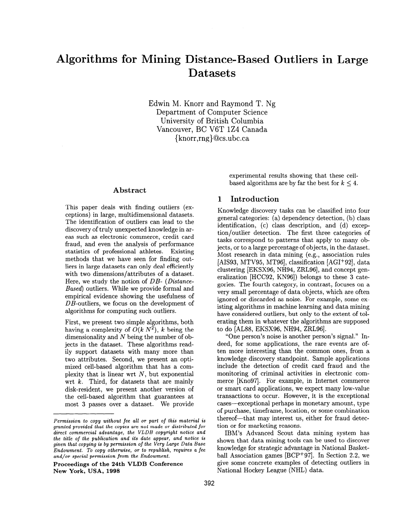
Cover for Algorithms for Mining Distance-Based Outliers in Large Datasets

Abstract

This paper deals with finding outliers (exceptions) in large, multidimensional datasets. The identification of outliers can lead to the discovery of truly unexpected knowledge in areas such as electronic commerce, credit card fraud, and even the analysis of performance statistics of professional athletes. Existing methods that we have seen for finding outliers in large datasets can only deal efficiently with two dimensions/attributes of a dataset. Here, we study the notion of DB- (Distance-Based) outliers. While we provide formal and empirical evidence showing the usefulness of DB-outliers, we focus on the development of algorithms for computing such outliers.

First, we present two simple algorithms, both having a complexity of O(k N²), k being the dimensionality and N being the number of objects in the dataset. These algorithms readily support datasets with many more than two attributes. Second, we present an optimized cell-based algorithm that has a complexity that is linear wrt N, but exponential wrt k. Third, for datasets that are mainly disk-resident, we present another version of the cell-based algorithm that guarantees at most 3 passes over a dataset. We provide experimental results showing that these cell-based algorithms are by far the best for k ≤ 4.

Topics

adaptive algorithms commerce credit card frauds optimization problems association rules efficient algorithm hard disks ebusiness empirical analysis

Keywords

distance-based outlier mining outlier detection index-based algorithms multidimensional indexing depth-based methods range search spatial data

1 Introduction
1.1 Related Work
1.2 Distance-Based Outliers and Contributions of this Paper
2 Justification for DB-Outliers
2.1 Properties of DB(p, D)-Outliers
2.2 Sample Runs Using NHL Statistics
3 Simple Algorithms for Finding All DB(p, D)-Outliers
3.1 Index-Based Algorithms
3.2 A Nested-Loop Algorithm
4 A Cell-Based Approach
4.1 Cell Structure and Properties in 2-D
4.2 Algorithm FindAllOutsM for MemoryResident Datasets
4.3 Complexity Analysis: The 2-D Case
4.4 Generalization to Higher Dimensions
4.5 Complexity Analysis: The Case for Higher Dimensions
5 DB-Outliers in Large, Disk-Resident Datasets
5.1 Handling Large, Disk-Resident Datasets: An Example
5.2 Algorithm FindAllOutsD Disk-Resident Datasets for
5.3 Analysis of Algorithm FindAllOutsD and Comparison with Algorithm NL
6 Empirical Behaviour of the Algorithms
6.1 Experimental Setup
6.2 Varying the Dataset Size
6.3 Varying the Value of p
6.4 Varying the Number of Dimensions and Cells
7 Conclusions
Acknowledgements
References

Knowls

Knowl 1 — Distance-Based Outlier (DB(p, D)-Outlier)
definition
Let $T$ be a dataset containing $N$ objects in a $k$ -dimensional space, and let $F(O, Q)$ be a metric distance function (such as Euclidean or weighted Euclidean distance) defining the distance between any pair of objects $O, Q \in T$ .

For parameters $p \in (0, 1)$ and $D > 0$ , an object $O \in T$ is defined as a $DB(p, D)$ -outlier if at least fraction $p$ of the objects in $T$ lie at a distance greater than $D$ from $O$ .

Equivalently, defining the $D$ -neighbourhood of $O$ as the set of objects within distance $D$ : $\{Q \in T \mid F(O, Q) \le D\}$ an object $O$ is a $DB(p, D)$ -outlier if and only if its $D$ -neighbourhood contains at most $M$ objects, where: $M = N(1 - p)$ Here, $M$ denotes the maximum allowable number of neighbours within distance $D$ for an object to remain classified as an outlier.
Knowl 2 — Multi-Dimensional Cell Grid Partitioning and Pruning Properties for DB-Outliers
model/method
To identify $DB(p, D)$ -outliers without performing all $O(N^2)$ pairwise distance comparisons, the $k$ -dimensional data space is quantized into hypercubical cells with side length: $l = \frac{D}{2\sqrt{k}}$

For any cell $C_{x_1, \dots, x_k}$ , its Layer 1 ( $L_1$ ) neighbours are defined as: $L_1(C_{x_1, \dots, x_k}) = \{ C_{u_1, \dots, u_k} \mid u_i = x_i \pm 1, \, \forall 1 \le i \le k \} \setminus \{ C_{x_1, \dots, x_k} \}$

Its Layer 2 ( $L_2$ ) neighbours are defined with thickness $x = \lceil 2\sqrt{k} - 1 \rceil$ as: $L_2(C_{x_1, \dots, x_k}) = \{ C_{u_1, \dots, u_k} \mid u_i = x_i \pm x, \, \forall 1 \le i \le k \} \setminus (L_1(C_{x_1, \dots, x_k}) \cup \{ C_{x_1, \dots, x_k} \})$

These dimensions yield the following distance properties:
1. Any two objects inside the same cell are separated by a distance of at most $\frac{D}{2}$ .
2. Any object in cell $C$ and any object in an $L_1$ neighbour of $C$ are separated by at most $D$ .
3. Any object in cell $C$ and any object in a cell outside $C \cup L_1(C) \cup L_2(C)$ are separated by strictly more than $D$ .
Letting $M = N(1 - p)$ be the maximum allowable neighbours for an outlier, the following cell-level classification rules hold:
- Red Cell: If the number of objects in $C$ satisfies $|C| > M$ , no object in $C$ is an outlier.
- Pink Cell: If $|C \cup L_1(C)| > M$ , no object in $C$ is an outlier.
- Yellow Cell: If $|C \cup L_1(C) \cup L_2(C)| \le M$ , every object in $C$ is an outlier.
Objects residing in uncoloured (white) cells that fail all three pruning tests must undergo object-by-object distance comparisons against objects in their $L_2$ neighbouring cells.
Knowl 3 — Memory-Resident Cell-Based Outlier Detection (Algorithm FindAllOutsM)
algorithm
Algorithm FindAllOutsM finds all $DB(p, D)$ -outliers when both the cell grid index and the dataset fit entirely in main memory. The algorithm quantizes objects into cells of length $l = D / (2\sqrt{k})$ , labels cells exceeding $M = N(1-p)$ objects as red, labels $L_1$ neighbours of red cells as pink, and filters remaining white cells by aggregating counts across $L_1$ and $L_2$ neighbours. White cells that cannot be pruned are evaluated tuple-by-tuple against tuples in their $L_2$ neighbouring cells, terminating evaluation for an object as soon as its $D$ -neighbour counter exceeds $M$ .
Input: Dataset $T$ with $N$ objects in $k$ dimensions, distance threshold $D$ , fraction $p$
Output: Set of all $DB(p, D)$ -outliers
$M \leftarrow N(1 - p)$
$l \leftarrow D / (2\sqrt{k})$
Initialize grid of cells $C_1, \dots, C_m$ with side length $l$
for $q \leftarrow 1$ to $m$ do
     $Count_q \leftarrow 0$
for each object $P \in T$ do
    Map $P$ to its corresponding cell $C_q$
    Store $P$ in $C_q$
     $Count_q \leftarrow Count_q + 1$
for $q \leftarrow 1$ to $m$ do
    if $Count_q > M$ then
        Label $C_q$ as red
for each red cell $C_r$ do
    for each cell $C \in L_1(C_r)$ do
        if $C$ is not red then
            Label $C$ as pink
for each non-empty uncoloured (white) cell $C_w$ do
     $Count_{w2} \leftarrow Count_w + \sum_{C_i \in L_1(C_w)} Count_i$
    if $Count_{w2} > M$ then
        Label $C_w$ as pink
    else
         $Count_{w3} \leftarrow Count_{w2} + \sum_{C_i \in L_2(C_w)} Count_i$
        if $Count_{w3} \le M$ then
            Mark all objects in $C_w$ as outliers
        else
            for each object $P \in C_w$ do
                 $Count_P \leftarrow Count_{w2}$
                for each object $Q \in \bigcup_{C_i \in L_2(C_w)} C_i$ do
                    if $dist(P, Q) \le D$ then
                         $Count_P \leftarrow Count_P + 1$
                        if $Count_P > M$ then
                            Break to next object $P$
                if $Count_P \le M$ then
                    Report $P$ as an outlier
The worst-case time complexity is $O(c^k + N)$ , where $c$ is a constant depending on $\sqrt{k}$ and the number of partitions per dimension, maintaining linear scaling with respect to $N$ .
Knowl 4 — Disk-Resident Cell-Based Outlier Detection (Algorithm FindAllOutsD)
algorithm
Algorithm FindAllOutsD detects all $DB(p, D)$ -outliers for large disk-resident datasets. It maintains only white and yellow tuples (tuples mapping to unresolved or fully outlying cells) in main memory, avoiding the need to buffer the entire dataset. In an initial pass, it quantizes objects to cells and records page references. It labels red, pink, and yellow cells, loads Class A pages (pages with white/yellow tuples), performs pairwise checks among loaded tuples, and subsequently reads Class B pages (pages with non-white tuples in $L_2$ of white cells) while re-reading necessary Class A pages.
Input: Disk-resident dataset $T$ of $N$ objects in $k$ dimensions, distance threshold $D$ , fraction $p$
Output: Set of all $DB(p, D)$ -outliers
$M \leftarrow N(1 - p)$
$l \leftarrow D / (2\sqrt{k})$
Initialize grid of cells $C_1, \dots, C_m$
for $q \leftarrow 1$ to $m$ do
     $Count_q \leftarrow 0$
for each object $P \in T$ from disk do
    Map $P$ to appropriate cell $C_q$ (do not store $P$ in memory)
     $Count_q \leftarrow Count_q + 1$
    Record that cell $C_q$ references the disk page of $P$
for $q \leftarrow 1$ to $m$ do
    if $Count_q > M$ then
        Label $C_q$ as red
for each red cell $C_r$ do
    for each cell $C \in L_1(C_r)$ do
        if $C$ is not red then
            Label $C$ as pink
for each non-empty white cell $C_w$ do
     $Count_{w2} \leftarrow Count_w + \sum_{C_i \in L_1(C_w)} Count_i$
    if $Count_{w2} > M$ then
        Label $C_w$ as pink
    else
         $Count_{w3} \leftarrow Count_{w2} + \sum_{C_i \in L_2(C_w)} Count_i$
        if $Count_{w3} \le M$ then
            Label $C_w$ as yellow
        else
             $Sum_w \leftarrow Count_{w2}$
for each disk page $i$ containing at least one white or yellow tuple do
    Read page $i$
    for each white or yellow cell $C_q$ having tuples in page $i$ do
        for each object $P$ in page $i$ mapped to $C_q$ do
            Store $P$ in $C_q$
             $Kount_P \leftarrow Sum_w$
for each non-empty white cell $C_w$ do
    for each white or yellow cell $C_L \in L_2(C_w)$ do
        for each object $P \in C_w$ (unmarked) do
            for each object $Q \in C_L$ do
                if $dist(P, Q) \le D$ then
                     $Kount_P \leftarrow Kount_P + 1$
                    if $Kount_P > M$ then
                        Mark $P$ as non-outlier
Report all objects in yellow cells as outliers
for each disk page $i$ containing tuples mapped to non-white/non-yellow $L_2$ neighbours of white cells do
    Read page $i$
    for each cell $C_q \in L_2(C_w)$ (non-white, non-yellow) having tuples in page $i$ do
        for each object $Q$ in page $i$ mapped to $C_q$ do
            for each non-empty white cell $C_w \in L_2(C_q)$ do
                for each object $P \in C_w$ (unmarked) do
                    if $dist(P, Q) \le D$ then
                         $Kount_P \leftarrow Kount_P + 1$
                        if $Kount_P > M$ then
                            Mark $P$ as non-outlier
for each object $P$ in each non-empty white cell do
    if $P$ is not marked as a non-outlier then
        Report $P$ as an outlier
Knowl 5 — Dataset Pass Bound for Algorithm FindAllOutsD
theoretical result
Let a dataset reside across $n = n_1 + n_2 + n_3$ pages on disk, partitioned into:
- Class A ( $n_1$ pages): pages containing at least one white or yellow tuple.
- Class B ( $n_2$ pages): pages containing no white/yellow tuples, but containing tuples mapped to non-white cells that are $L_2$ neighbours of white cells.
- Class C ( $n_3$ pages): all remaining pages.
Algorithm FindAllOutsD requires at most 3 passes over the dataset on disk.

The initial mapping phase performs exactly 1 full pass ( $n$ page reads). In the object-pairwise phase, the algorithm reads all Class A pages ( $n_1$ ), followed by all Class B pages ( $n_2$ ), and finally re-reads Class A pages ( $n_1$ ), resulting in at most $2n_1 + n_2 \le 2n$ additional page reads. The total number of page reads is bounded by $n + 2n_1 + n_2 \le 3n$ .

Furthermore, if $n_1 \le n_3$ , then $2n_1 + n_2 \le n_1 + n_2 + n_3 = n$ , which guarantees that the total I/O cost does not exceed 2 passes over the dataset.
Knowl 6 — Block-Oriented Nested-Loop Outlier Detection (Algorithm NL)
algorithm
Algorithm NL computes all $DB(p, D)$ -outliers without constructing spatial index or cell grid structures. Given a buffer of size $B\%$ of the dataset size, the buffer is split into two halves: the first array and the second array. A block of tuples is loaded into the first array, and pairwise distances are computed within the block and against blocks streamed through the second array. For each tuple $t_i$ in the first array, neighbour counting stops immediately once the count exceeds $M = N(1-p)$ .
Input: Dataset $T$ of $N$ tuples, distance threshold $D$ , fraction $p$ , memory buffer size $B\%$
Output: Set of all $DB(p, D)$ -outliers
$M \leftarrow N(1 - p)$
Divide buffer into two arrays of equal size
Load initial block of tuples from $T$ into the first array
for each tuple $t_i$ in the first array do
     $count_i \leftarrow 0$
    for each tuple $t_j$ in the first array do
        if $dist(t_i, t_j) \le D$ then
             $count_i \leftarrow count_i + 1$
            if $count_i > M$ then
                Mark $t_i$ as non-outlier and proceed to next $t_i$
while blocks remain to be compared against the first array do
    Fill second array with another block (saving an unbuffered block for last)
    for each unmarked tuple $t_i$ in the first array do
        for each tuple $t_j$ in the second array do
            if $dist(t_i, t_j) \le D$ then
                 $count_i \leftarrow count_i + 1$
                if $count_i > M$ then
                    Mark $t_i$ as non-outlier and proceed to next $t_i$
for each unmarked tuple $t_i$ in the first array do
    Report $t_i$ as an outlier
if second array has previously served as the first array then
    Stop
else
    Swap first and second array designations and continue comparing remaining blocks
The time complexity of Algorithm NL is $O(k N^2)$ , where $k$ is the dimensionality and $N$ is the dataset size.
Knowl 7 — I/O Complexity and Dataset Passes of Algorithm NL
theoretical result
Let a dataset be partitioned into $n = \lceil 100/B \rceil$ logical blocks, where $B$ is the percentage of total dataset size available in the memory buffer (with the buffer divided into two halves to support block nested-loop comparisons).

Under Algorithm NL:
1. The total number of block reads required is: $\text{Total Block Reads} = n + (n - 2)(n - 1)$
2. The total number of passes over the dataset is: $\text{Passes} = \frac{n + (n - 2)(n - 1)}{n} = \frac{n^2 - 2n + 2}{n} = n - 2 + \frac{2}{n} \ge n - 2$
For datasets where $n$ is large (e.g., when $n = 10$ , requiring 8 passes), Algorithm NL requires significantly more disk passes than the cell-based disk algorithm FindAllOutsD, which is guaranteed to require at most 3 passes.

Knowl 8 — Dimensionality Crossover and Scalability of Cell-Based vs. Nested-Loop Algorithms

data/table

The execution times (CPU time plus I/O time in seconds) of the cell-based algorithm (CS) and the block nested-loop algorithm (NL) were evaluated on disk-resident synthetic datasets mirroring NHL statistics across dimensions $k \in \{3, 4, 5\}$ and sizes $N \in \{100\text{k}, 500\text{k}, 2\text{M}\}$ with $p = 0.9999$ on an UltraSPARC-1 machine (128 MB RAM).

	3-D		4-D		5-D
$N$	$\text{CS}(10^3)$	$\text{NL}$	$\text{CS}(10^4)$	$\text{NL}$	$\text{CS}(10^5)$	$\text{CS}(8^5)$	$\text{CS}(6^5)$	$\text{NL}$
100,000	10.77	93.96	23.32	45.79	93.40	217.04	205.63	17.30
500,000	57.10	490.62	114.00	223.51	695.37	997.11	1061.33	148.44
2,000,000	253.90	2332.10	606.56	1421.16	>2147	>2147	>2147	1555.78

In the table, $\text{CS}(m_i^k)$ denotes the cell structure with $m_i$ partitions per dimension, yielding $m = m_i^k$ cells.

The results demonstrate:

For $k = 3$ , CS outperforms NL by nearly an order of magnitude (e.g., $253.90\text{ s}$ vs. $2332.10\text{ s}$ for $N = 2\text{M}$ ) because CS scales linearly with $N$ .
For $k = 4$ , CS remains substantially faster than NL across all dataset sizes.
For $k = 5$ , NL outperforms CS across all tested cell granularities ( $10^5, 8^5, 6^5$ ), because the exponential growth in the number of cells ( $O(c^k)$ ) dominates CS processing time. Thus, CS is preferred for $k \le 4$ , whereas NL is the preferred algorithm for $k \ge 5$ .

Knowl 9 — Inefficiency of Multidimensional Index Structures for DB-Outlier Detection
empirical result
Evaluating multidimensional spatial index structures—specifically memory-resident $k$ -d trees (KD) and disk-based R-trees (RT)—shows that index-based outlier detection is uncompetitive with cell-based (CS) and block nested-loop (NL) algorithms:
- In 3-D memory-resident experiments with $p = 0.9995$ , KD required $3.14\text{ s}$ for $N = 20,000$ (compared to $0.32\text{ s}$ for CS and $1.02\text{ s}$ for NL), and $104.28\text{ s}$ for $N = 100,000$ (compared to $1.43\text{ s}$ for CS and $27.67\text{ s}$ for NL). The time required merely to construct the $k$ -d tree index exceeded the total runtime of CS and NL.
- In 3-D disk-resident experiments, building the R-tree index alone took at least 10 times longer than the complete execution time of CS.
- Multidimensional range query search complexity in $k$ dimensions has a lower bound of $\Omega(N^{1 - 1/k})$ , which rapidly approaches $O(N)$ sequential search as $k$ increases, making total outlier search cost $O(k N^2)$ on top of index construction overhead.
Knowl 10 — Unification of Classical Statistical Outlier Definitions by DB-Outliers
theoretical result
The $DB(p, D)$ -outlier framework unifies classical distribution-based outlier definitions. Formally, $DB(p, D)$ unifies an outlier definition $Def$ if there exist fixed parameters $p_0 \in (0, 1)$ and $D_0 > 0$ such that an object $O$ is an outlier according to $Def$ if and only if $O$ is a $DB(p_0, D_0)$ -outlier.

Concrete unifications include:
1. Normal Distribution: Let $Def_{Normal}$ define $t$ as an outlier in a normal distribution with mean $\mu$ and standard deviation $\sigma$ if $\frac{|t - \mu|}{\sigma} > 3$ . $DB(p, D)$ unifies $Def_{Normal}$ with: $p_0 = 0.9988, \quad D_0 = 0.13\sigma$
2. Poisson Distribution: Let $Def_{Poisson}$ define $t$ as an outlier in a Poisson distribution with parameter $\mu = 3.0$ if $t \ge 8$ . $DB(p, D)$ unifies $Def_{Poisson}$ with: $p_0 = 0.9892, \quad D_0 = 1$
Analogous unifications hold for Student's $t$ -distributions and linear regression outlier models.

Coverage note — None was omitted; the extracted knowls cover all contributed definitions, algorithmic implementations (NL, FindAllOutsM, FindAllOutsD), cell pruning properties, I/O guarantees, and empirical performance benchmarks across dimensions and dataset sizes.

References

1.A. Arning, R. Agrawal, and P. Raghavan. A linear method for deviation detection in large databases. In Proc. KDD, pages 164–169, 1996.
2.R. Agrawal, S. Ghosh, T. Imielinski, B. Iyer, and A. Swami. An interval classifier for database mining applications. In Proc. 18th VLDB, pages 560–573, 1992.
3.R. Agrawal, T. Imielinski, and A. Swami. Mining association rules between sets of items in large databases. In Proc. ACM SIGMOD, pages 207–216, 1993.
4.D. Angluin and P. Laird. Learning from noisy examples. Machine Learning, 2(4):343–370, 1988.
5.I. S. Bhandari, E. Colet, J. Parker, Z. Pines, R. Pratap, and K. Ramanujam. Advanced scout: Data mining and knowledge discovery in NBA data. Data Mining and Knowledge Discovery, 1(1):121–125, 1997.
6.J. L. Bentley. Multidimensional binary search trees used for associative searching. CACM, 18(9):509–517, 1975.
7.V. Barnett and T. Lewis. Outliers in Statistical Data. John Wiley, 3rd edition, 1994.
8.M. Ester, H.-P. Kriegel, J. Sander, and X. Xu. A density-based algorithm for discovering clusters in large spatial databases with noise. In Proc. KDD, pages 226–231, 1996.
9.D. Freedman, R. Pisani, and R. Purves. Statistics. W.W. Norton, New York, 1978.
10.R. Guttmann. A dynamic index structure for spatial searching. In Proc. ACM SIGMOD, pages 47–57, 1984.
11.D. Hawkins. Identification of Outliers. Chapman and Hall, London, 1980.
12.J. Han, Y. Cai, and N. Cercone. Knowledge discovery in databases: An attribute-oriented approach. In Proc. 18th VLDB, pages 547–559, 1992.
13.J. Hellerstein, E. Koutsoupias, and C. Papadimitriou. On the analysis of indexing schemes. In Proc. PODS, pages 249–256, 1997.
14.R. A. Johnson and D. W. Wichern. Applied Multivariate Statistical Analysis. Prentice-Hall, 3rd edition, 1992.
15.E. M. Knorr and R. T. Ng. Finding aggregate proximity relationships and commonalities in spatial data mining. IEEE Transactions on Knowledge and Data Engineering, 8(6):884–897, 1996.
16.E. M. Knorr and R. T. Ng. A unified notion of outliers: Properties and computation. In Proc. KDD, pages 219–222, 1997. An extended version of this paper appears as: E. M. Knorr and R.T. Ng. A Unified Approach for Mining Outliers. In Proc. 7th CASCON, pages 236–248, 1997.
17.E. M. Knorr. On digital money and card technologies. Technical Report 97-02, University of British Columbia, 1997.
18.H. Mannila and H. Toivonen. Discovering generalized episodes using minimal occurrences. In Proc. KDD, pages 146–151, 1996.
19.H. Mannila, H. Toivonen, and A. Verkamo. Discovering frequent episodes in sequences. In Proc. KDD, pages 210–215, 1995.
20.R. Ng and J. Han. Efficient and effective clustering methods for spatial data mining. In Proc. 20th VLDB, pages 144–155, 1994.
21.F. Preparata and M. Shamos. Computational Geometry: an Introduction. Springer-Verlag, 1988.
22.I. Ruts and P. Rousseeuw. Computing depth contours of bivariate point clouds. Computational Statistics and Data Analysis, 23:153–168, 1996.
23.H. Samet. The Design and Analysis of Spatial Data Structures. Addison-Wesley, 1990.
24.T. Zhang, R. Ramakrishnan, and M. Livny. BIRCH: An efficient data clustering method for very large databases. In Proc. ACM SIGMOD, pages 103–114, 1996.

Citation

MLA

Knorr, E. M., and R. T. Ng. “Algorithms for Mining Distance-Based Outliers in Large Datasets”. Very Large Data Bases, 1998, pp. 392–403, http://citeseerx.ist.psu.edu/viewdoc/summary?doi=10.1.1.55.8026.

APA

Knorr, E. M., & Ng, R. T. (1998). Algorithms for Mining Distance-Based Outliers in Large Datasets. Very Large Data Bases, 392–403. http://citeseerx.ist.psu.edu/viewdoc/summary?doi=10.1.1.55.8026

Chicago

Knorr, E. M., and R. T. Ng. 1998. “Algorithms for Mining Distance-Based Outliers in Large Datasets”. Very Large Data Bases, 392–403. http://citeseerx.ist.psu.edu/viewdoc/summary?doi=10.1.1.55.8026.

Harvard

Knorr, E.M. and Ng, R.T. (1998) “Algorithms for Mining Distance-Based Outliers in Large Datasets”, Very Large Data Bases, pp. 392–403. Available at: http://citeseerx.ist.psu.edu/viewdoc/summary?doi=10.1.1.55.8026.

Vancouver

1. Knorr EM, Ng RT (1998) Algorithms for Mining Distance-Based Outliers in Large Datasets. Very Large Data Bases 392–403

BibTeX

@article{knorr1998algorithms,
  title = {Algorithms for Mining Distance-Based Outliers in Large Datasets},
  author = {Knorr, Edwin M. and Ng, Raymond T.},
  year = {1998},
  journal = {Very Large Data Bases},
  pages = {392-403},
  url = {http://citeseerx.ist.psu.edu/viewdoc/summary?doi=10.1.1.55.8026}
}

Metadata:DOI registry

Access the Paper

This paper is available from its original source. Click below to access the PDF.

Open PDF

Algorithms for Mining Distance-Based Outliers in Large Datasets

Abstract

Topics

Keywords

Table of Contents

Knowls

Knowl 1 — Distance-Based Outlier (DB(p, D)-Outlier)

Knowl 2 — Multi-Dimensional Cell Grid Partitioning and Pruning Properties for DB-Outliers

Knowl 3 — Memory-Resident Cell-Based Outlier Detection (Algorithm FindAllOutsM)

Knowl 4 — Disk-Resident Cell-Based Outlier Detection (Algorithm FindAllOutsD)

Knowl 5 — Dataset Pass Bound for Algorithm FindAllOutsD

Knowl 6 — Block-Oriented Nested-Loop Outlier Detection (Algorithm NL)

Knowl 7 — I/O Complexity and Dataset Passes of Algorithm NL

Knowl 8 — Dimensionality Crossover and Scalability of Cell-Based vs. Nested-Loop Algorithms

Knowl 9 — Inefficiency of Multidimensional Index Structures for DB-Outlier Detection

Knowl 10 — Unification of Classical Statistical Outlier Definitions by DB-Outliers

References

Citation

BibTeX

Access the Paper