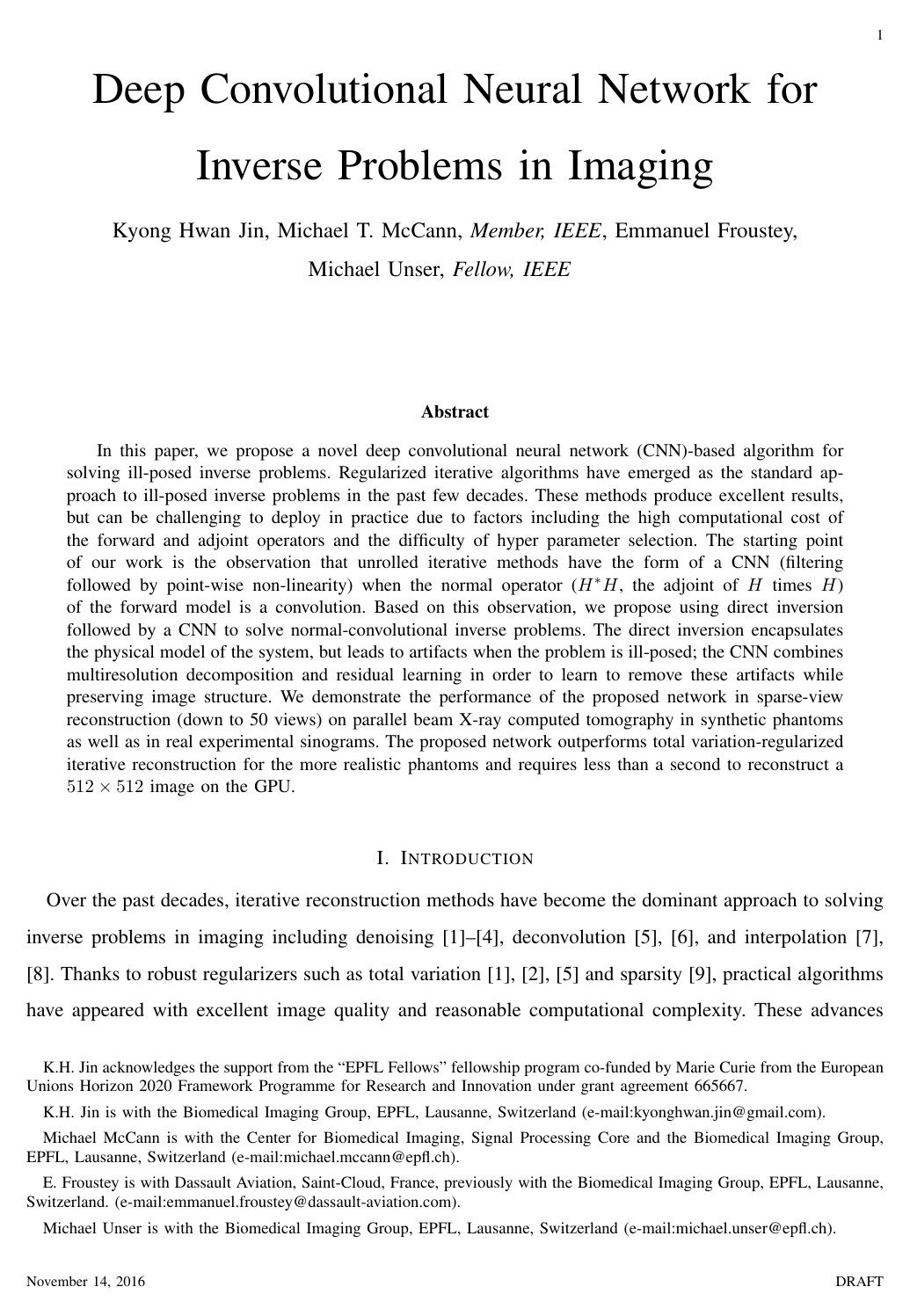
Deep Convolutional Neural Network for Inverse Problems in Imaging

Kyong Hwan JinMichael T. McCannEmmanuel FrousteyMichael Unser

article2016IEEE Transactions on Image Processing2,472 citationsIEEE Signal Processing Society Best Paper Award

Proposes a framework combining direct physical inversion with a residual convolutional neural network to solve ill-posed imaging inverse problems, achieving superior quality over standard iterative reconstruction while recovering sparse-view computed tomography images in sub-second speeds.

Listen

Medical imaging modalities such as X-ray computed tomography face an inherent trade-off between acquisition time and image quality. Short acquisition times or sparse-view scans reduce harmful radiation exposure and patient motion artifacts, but direct mathematical reconstruction yields severe streaking artifacts. While iterative reconstruction methods produce high-quality images, they suffer from high computational demands and long reconstruction runtimes that limit their routine clinical adoption.

The article sets out to develop and evaluate a deep learning reconstruction framework that combines direct physical inversion with a deep convolutional neural network to solve imaging inverse problems rapidly while preserving image quality.

The researchers established a mathematical framework showing that a broad class of imaging problems can be formulated as convolutional operations, enabling the use of convolutional neural networks. Based on this, they designed a system named FBPConvNet, which performs a fast, standard filtered back projection to provide an initial physical estimate and then applies a multiresolution neural network based on the U-Net architecture with residual learning to remove artifacts. The approach was evaluated on sparse-view computed tomography using three datasets: a synthetic geometric ellipsoid dataset, 500 clinical in-vivo scans from the Mayo Clinic, and 377 experimental scans of a rat brain collected from a synchrotron light source.

The evaluation yielded several key findings. First, FBPConvNet consistently outperformed state-of-the-art total variation iterative reconstruction on realistic clinical and biological datasets, achieving higher signal-to-noise ratios (such as 36.15 dB versus 31.92 dB on clinical data at 143 views). Second, the neural network effectively preserved fine anatomical textures and detailed structures, avoiding the unnatural, oversmoothed cartoon-like artifacts typical of total variation methods. Third, the proposed method reconstructed a 512-by-512 image in under one second on a standard graphics processing unit, representing a massive speedup compared to iterative methods that required approximately seven minutes per image. Finally, the iterative method maintained an advantage only on idealized, piecewise-constant synthetic phantoms where total variation regularization is mathematically optimal.

These findings indicate that deep learning combined with physical domain models can substantially reduce patient radiation exposure by enabling reconstructions from sparse views (subsampled by up to twenty times) without sacrificing diagnostic texture quality. The dramatic reduction in processing time makes high-quality sparse reconstruction practical for real-time and high-throughput clinical workflows.

Organizations evaluating this approach should consider piloting direct-inversion neural networks in imaging pipelines where rapid processing and low-dose scans are critical. Before clinical deployment, future work should develop unified strategies for heterogeneous datasets and expand network architectures to support complex-valued data required for modalities such as magnetic resonance imaging.

A primary limitation of the method is its lack of transferability across varying scan configurations; a model trained on a specific downsampling factor must be retrained to process scans acquired with different numbers of views. While confidence in the experimental performance on computed tomography is high, testing remains constrained to two-dimensional slices, and careful validation on larger, varied clinical cohorts is necessary prior to production deployment.

Cover for Deep Convolutional Neural Network for Inverse Problems in Imaging

Abstract

In this paper, we propose a novel deep convolutional neural network (CNN)-based algorithm for solving ill-posed inverse problems. Regularized iterative algorithms have emerged as the standard approach to ill-posed inverse problems in the past few decades. These methods produce excellent results, but can be challenging to deploy in practice due to factors including the high computational cost of the forward and adjoint operators and the difficulty of hyper parameter selection. The starting point of our work is the observation that unrolled iterative methods have the form of a CNN (filtering followed by point-wise non-linearity) when the normal operator (H*H, the adjoint of H times H) of the forward model is a convolution. Based on this observation, we propose using direct inversion followed by a CNN to solve normal-convolutional inverse problems. The direct inversion encapsulates the physical model of the system, but leads to artifacts when the problem is ill-posed; the CNN combines multiresolution decomposition and residual learning in order to learn to remove these artifacts while preserving image structure. We demonstrate the performance of the proposed network in sparse-view reconstruction (down to 50 views) on parallel beam X-ray computed tomography in synthetic phantoms as well as in real experimental sinograms. The proposed network outperforms total variation-regularized iterative reconstruction for the more realistic phantoms and requires less than a second to reconstruct a 512 x 512 image on GPU.

Table of Contents

  • I Introduction
  • II Inverse Problems with Shift-Invariant Normal Operators
  • II-A Theory
  • II-B Direct Inversion
  • II-C Iterative Inversion
  • III Proposed Method: FBPConvNet
  • III-A Filtered Back Projection
  • III-B Deep Convolutional Neural Network Design
  • IV Experiments and results
  • IV-A Data Preparation
  • IV-B Training Procedure
  • V Experimental Results
  • V-A Ellipsoidal Dataset
  • V-B Biomedical Dataset
  • V-C Experimental Dataset
  • VI Discussion
  • VII Conclusion
  • References

Knowls

  1. Knowl 1 — FBPConvNet Reconstruction Framework

    model/method

    The FBPConvNet framework solves ill-posed linear inverse problems of the form g=Hfg = H f, where the forward operator HH has a shift-invariant normal operator HHH^* H, by combining a physics-based direct inversion with a deep convolutional neural network (CNN).

    Instead of learning an end-to-end mapping directly from measurement space (which requires neural networks to learn coordinate transformations like the Radon backprojection geometry), FBPConvNet applies an analytical, approximate direct inversion (such as Filtered Backprojection, FBP) to map measurements gg into an initial reconstruction in the image domain:

    finitial=FBP(g)f_{\text{initial}} = \text{FBP}(g)

    This initial estimate contains the correct underlying geometry but suffers from severe undersampling and noise artifacts. A deep convolutional network with a multi-scale U-Net architecture and a global residual skip connection is trained to estimate and remove these artifacts:

    frecon=finitial+CNN(finitial)f_{\text{recon}} = f_{\text{initial}} + \text{CNN}(f_{\text{initial}})

    The network is trained using pairs of low-view (sparse) FBP images and high-view (full-acquisition) FBP images as input and target pairs, enabling training on real scanner data without requiring synthetic or oracle ground truths.

  2. Knowl 2 — Shift-Invariance of Normal Operators in Imaging Forward Models

    theoretical result

    Let F\mathcal{F} denote the continuous Fourier transform, T:L2(Ω)L2(Ω)T: L_2(\Omega) \to L_2(\Omega) be a linear isometry, Mm:L2(Ω)L2(Ω)M_m: L_2(\Omega) \to L_2(\Omega) be a multiplication operator defined by Mm{f}(x)=m(x)f(x)M_m\{f\}(x) = m(x)f(x) for a continuous bounded function mL2(Ω)m \in L_2(\Omega), and Φϕ:L2(Ω1)L2(Ω2)\Phi_\phi: L_2(\Omega_1) \to L_2(\Omega_2) be a reversible change of variables defined by Φϕ{f}(x)=f(ϕ(x))\Phi_\phi\{f\}(x) = f(\phi(x)) with Jacobian matrix JϕJ_\phi.

    If a linear forward operator H:L2(Rd1)L2(Ω)H: L_2(\mathbb{R}^{d_1}) \to L_2(\Omega) can be factored as:

    H=TMmΦϕ1FH = T M_m \Phi_\phi^{-1} \mathcal{F}

    then its normal operator HHH^* H is a spatial convolution operator HhH_h, defined by:

    HH=FMh^FH^* H = \mathcal{F}^* M_{\hat{h}} \mathcal{F}

    where the Fourier transform of the convolution kernel h^\hat{h} is given by:

    h^(ω)=detJϕ(ω)(Φϕm(ω)2)\hat{h}(\omega) = |\det J_\phi(\omega)| \cdot (\Phi_\phi |m(\omega)|^2)

    In the discrete domain, if Hd=SHcQH_d = S H_c Q where HcH_c satisfies this factorization, SS denotes sampling, QQ denotes interpolation, and HcQfH_c Q f is bandlimited, HdHdH_d^* H_d is likewise a discrete convolution. For the continuous 2D Radon transform RR, RRR^* R is a convolution with frequency response h^(ω)=1ω2\hat{h}(\omega) = \frac{1}{\|\omega\|_2}.

  3. Knowl 3 — Connection Between Unrolled Proximal Iterative Solvers and Deep CNNs

    theoretical result

    Consider a regularized linear inverse problem in synthesis form:

    argminayHWa22+λa1\arg\min_a \|y - H W a\|_2^2 + \lambda \|a\|_1

    where yRNyy \in \mathbb{R}^{N_y} denotes measurements, HRNy×NxH \in \mathbb{R}^{N_y \times N_x} is the forward operator, WRNx×NaW \in \mathbb{R}^{N_x \times N_a} is a shift-invariant frame synthesis operator (such as a multi-channel wavelet transform), aRNaa \in \mathbb{R}^{N_a} is the sparse coefficient vector, and x=Wax = W a is the desired image.

    Applying the Iterative Shrinkage-Thresholding Algorithm (ISTA) yields the iterate update:

    ak+1=Sλ/L(1LWHy+(I1LWHHW)ak)a^{k+1} = \mathcal{S}_{\lambda / L}\left( \frac{1}{L} W^* H^* y + \left(I - \frac{1}{L} W^* H^* H W\right) a^k \right)

    where Sθ(u)=sign(u)max(uθ,0)\mathcal{S}_\theta(u) = \text{sign}(u)\max(|u|-\theta, 0) is the soft-thresholding operator applied component-wise and Lλmax(WHHW)L \le \lambda_{\max}(W^* H^* H W) is the Lipschitz constant.

    When the normal operator HHH^* H is a convolution and WW is a convolution bank, the term (I1LWHHW)(I - \frac{1}{L} W^* H^* H W) acts as a multi-channel convolutional filter, 1LWHy\frac{1}{L} W^* H^* y acts as an additive bias, and Sλ/L\mathcal{S}_{\lambda / L} acts as a pointwise non-linear activation. An unrolled sequence of such iterations is structurally isomorphic to a deep feedforward convolutional neural network with inter-layer convolutions, biases, and non-linearities.

  4. Knowl 4 — Residual Multiscale U-Net Architecture for FBP Artifact Removal

    model/method

    The convolutional neural network in FBPConvNet processes a single-channel initial FBP reconstruction (512×512512 \times 512) via a modified U-Net architecture incorporating global residual learning:

    1. Contraction (Analysis) Path: Four downsampling stages. Each stage contains two successive 3×33 \times 3 convolutional layers (with batch normalization and ReLU activation), followed by 2×22 \times 2 max pooling with stride 2. Across the four levels, spatial resolution decreases dyadically (512×512256×256128×12864×6432×32512 \times 512 \to 256 \times 256 \to 128 \times 128 \to 64 \times 64 \to 32 \times 32), while channel capacity scales from 64 to 128, 256, 512, and 1024.
    2. Expansion (Synthesis) Path: Four upsampling stages. Each stage uses a 3×33 \times 3 transposed convolution with stride 2 (plus batch normalization and ReLU) to double spatial dimensions and halve channel depth, concatenates the resulting maps with high-resolution skip connections from the matching contraction level, and applies two successive 3×33 \times 3 convolutions (with batch normalization and ReLU).
    3. Output Layer: A 1×11 \times 1 convolutional layer reduces the final 64 channels to a single-channel image.
    4. Global Skip Connection: An identity skip connection adds the initial FBP input directly to the network's output, requiring the network to learn only the residual artifact pattern:

    x^=xFBP+N(xFBP)\hat{x} = x_{\text{FBP}} + \mathcal{N}(x_{\text{FBP}})

    1. Zero Padding: Zero-padding is used across all 3×33 \times 3 convolutions to ensure that feature maps do not shrink after filtering.
  5. Knowl 5 — Direct Inversion Formulas for Normal-Convolutional Forward Operators

    equation

    For an inverse problem g=Hfg = H f where H=TMmΦϕ1FH = T M_m \Phi_\phi^{-1} \mathcal{F} satisfies shift-invariance of the normal operator HHH^* H, exact continuous direct inversion can be implemented in two equivalent forms:

    1. Reconstruction-Space Filtering: Performing backprojection followed by deconvolution with an inverse filter WhW_h:

    f=WhHgf = W_h H^* g

    where WhW_h has Fourier frequency response:

    w^h(ω)=1detJϕ(ω)Φϕm(ω)2\hat{w}_h(\omega) = \frac{1}{|\det J_\phi(\omega)| \cdot \Phi_\phi |m(\omega)|^2}

    1. Measurement-Space Filtering (Filtered Backprojection): Filtering in the transform domain of TT prior to backprojecting:

    f=HTMhTgf = H^* T M_h T^* g

    where MhM_h is a multiplication operator defined by:

    h(ω)=1detJϕ(ω)m(ω)2h(\omega) = \frac{1}{|\det J_\phi(\omega)| \cdot |m(\omega)|^2}

    For 2D computed tomography, the first formulation applies a 2D filter with frequency magnitude ω2\|\omega\|_2 to the backprojected image, whereas the second applies a 1D ramp filter with magnitude ω|\omega| to each projection view prior to backprojection.

  6. Knowl 6 — Sparse-View CT Reconstruction Performance on Biomedical and Synchrotron Datasets

    data/table

    Reconstruction quality was evaluated on sparse-view parallel-beam X-ray CT against Filtered Backprojection (FBP) and a Total Variation (TV) regularized ADMM baseline. Performance was measured by Signal-to-Noise Ratio (SNR in dB):

    SNR=maxa,bR20log10x2x(ax^+b)2\text{SNR} = \max_{a,b \in \mathbb{R}} 20 \log_{10} \frac{\|x\|_2}{\|x - (a \hat{x} + b)\|_2}

    where xx is the full-view reference FBP reconstruction and x^\hat{x} is the test reconstruction.

    Two realistic datasets were tested:

    • Biomedical Dataset: 500 in-vivo human CT slices from the Mayo Clinic Low-Dose CT Grand Challenge (tested on 25 slices from an unseen subject) with 143 views (×7\times 7 downsampling) and 50 views (×20\times 20 downsampling).
    • TOMCAT Synchrotron Dataset: 377 real rat-brain CT slices from the Paul Scherrer Institute (tested on 25 slices separated by a 25-slice gap from training data) with 145 views (×5\times 5 downsampling) and 51 views (×14\times 14 downsampling).
    Dataset Subsampling FBP TV FBPConvNet
    Biomedical 143 views (×7\times 7) 24.97 dB 31.92 dB 36.15 dB
    Biomedical 50 views (×20\times 20) 13.52 dB 25.20 dB 28.83 dB
    TOMCAT Rat Brain 145 views (×5\times 5) 5.38 dB 8.25 dB 11.34 dB
    TOMCAT Rat Brain 51 views (×14\times 14) 3.29 dB 7.25 dB 8.85 dB

    On realistic datasets with intricate textural features, FBPConvNet outperforms TV regularization by 3.6--4.2 dB at moderate subsampling and 1.6--3.6 dB at severe subsampling, avoiding the cartoon-like blocky artifacts characteristic of TV.

  7. Knowl 7 — Reconstruction Comparison on Piecewise-Constant Synthetic Phantoms

    data/table

    On a synthetic dataset of 500 piecewise-constant random ellipse phantoms (tested on 25 holdout images), Total Variation (TV) regularized iterative reconstruction outperformed FBPConvNet across both 143 views (×7\times 7 subsampling) and 50 views (×20\times 20 subsampling):

    Subsampling FBP TV FBPConvNet
    143 views (×7\times 7) 16.09 dB 29.48 dB 28.96 dB
    50 views (×20\times 20) 8.44 dB 27.69 dB 23.84 dB

    Because the underlying synthetic images strictly adhere to the piecewise-constant prior assumed by total variation minimization, TV regularization acts as an optimal estimator for this class, whereas FBPConvNet retains minor residual streak artifacts.

  8. Knowl 8 — Computational Latency of FBPConvNet versus Iterative TV Reconstruction

    empirical result

    For a 512×512512 \times 512 image reconstruction from sparse-view projections, FBPConvNet requires under one second of total computation time:

    • Filtered Backprojection (FBP) step: 200 ms\sim 200\text{ ms}
    • CNN inference on an NVIDIA Titan Black GPU: 200300 ms200\text{--}300\text{ ms}
    • Total processing latency: <1 s< 1\text{ s}

    In comparison, the TV-regularized ADMM iterative baseline requires approximately 7 minutes per slice on the same data once its regularization hyperparameter has been pre-selected.

  9. Knowl 9 — Lack of Transfer Across Subsampling Ratios and Scanner Geometries

    limitation

    FBPConvNet does not generalize across varying subsampling factors or acquisition geometries without retraining. When an FBPConvNet trained on 7-times subsampled sinograms (143 views) is evaluated on inputs generated from 20-times subsampled sinograms (50 views), the network fails to eliminate severe streaking artifacts. Reconstructing data with different sinogram dimensions, view counts, or downsampling factors requires training dedicated network weights for each configuration.

  10. Knowl 10 — Training Configuration and Hyperparameters for FBPConvNet

    experimental setup

    FBPConvNet was implemented in MatConvNet and trained using low-view FBP reconstructions as network inputs and corresponding full-view FBP reconstructions as target outputs under the following protocol:

    • Optimization: Stochastic gradient descent with momentum set to 0.99.
    • Batch Size: 1.
    • Learning Rate: Decreased logarithmically from 10210^{-2} to 10310^{-3} over training.
    • Gradient Clipping: Gradients were clipped to a maximum magnitude of 10210^{-2} to avoid divergence.
    • Data Augmentation: Random horizontal and vertical flipping.
    • Training Duration: 101 iterations (approximately 15 hours on an NVIDIA Titan Black GPU).
    • Intensity Scaling: Image pixel values were scaled into the range [0,550][0, 550].

Coverage note — None was omitted; all theoretical characterizations of shift-invariant normal operators, model architectures, iterative algorithm connections, empirical evaluations on synthetic and real datasets, computational latencies, and limitations were captured.

References

  1. 1.L. I. Rudin, S. Osher, and E. Fatemi, “Nonlinear total variation based noise removal algorithms,” Physica D: Nonlinear Phenomena, vol. 60, no. 1, pp. 259–268, 1992.
  2. 2.A. Chambolle, “An algorithm for total variation minimization and applications,” J. Math. imaging and vision, vol. 20, no. 1-2, pp. 89–97, 2004.
  3. 3.S. G. Chang, B. Yu, and M. Vetterli, “Adaptive wavelet thresholding for image denoising and compression,” IEEE transactions on image processing, vol. 9, no. 9, pp. 1532–1546, 2000.
  4. 4.F. Luisier, T. Blu, and M. Unser, “A new SURE approach to image denoising: Interscale orthonormal wavelet thresholding,” IEEE Transactions on image processing, vol. 16, no. 3, pp. 593–606, 2007.
  5. 5.T. F. Chan and C.-K. Wong, “Total variation blind deconvolution,” IEEE transactions on Image Processing, vol. 7, no. 3, pp. 370–375, 1998.
  6. 6.D. Krishnan and R. Fergus, “Fast image deconvolution using hyper-Laplacian priors,” in Advances in Neural Information Processing Systems, 2009, pp. 1033–1041.
  7. 7.P. Thevenaz, T. Blu, and M. Unser, “Interpolation revisited [medical images application],” IEEE Transactions on medical imaging, vol. 19, no. 7, pp. 739–758, 2000.
  8. 8.M. Bertalmio, G. Sapiro, V. Caselles, and C. Ballester, “Image inpainting,” in Proceedings of the 27th annual conference on Computer graphics and interactive techniques. ACM Press/Addison-Wesley Publishing Co., 2000, pp. 417–424.
  9. 9.R. Tibshirani, “Regression shrinkage and selection via the lasso,” Journal of the Royal Statistical Society. Series B (Methodological), pp. 267–288, 1996.
  10. 10.H. Jung, K. Sung, K. S. Nayak, E. Y. Kim, and J. C. Ye, “k-t FOCUSS: A general compressed sensing framework for high resolution dynamic MRI,” Magnetic Resonance in Medicine, vol. 61, no. 1, pp. 103–116, Jan. 2009.
  11. 11.S. G. Lingala, Y. Hu, E. DiBella, and M. Jacob, “Accelerated Dynamic MRI Exploiting Sparsity and Low-Rank Structure: k-t SLR,” IEEE Transactions on Medical Imaging, vol. 30, no. 5, pp. 1042–1054, May 2011.
  12. 12.M. McGaffin and J. Fessler, “Alternating dual updates algorithm for X-ray CT reconstruction on the GPU,” IEEE Transactions on Computational Imaging, vol. 1, no. 3, pp. 186–199, Sep. 2015.
  13. 13.M. T. McCann, M. Nilchian, M. Stampanoni, and M. Unser, “Fast 3D reconstruction method for differential phase contrast X-ray CT,” Opt. Express, vol. 24, no. 13, pp. 14 564–14 581, Jun 2016.
  14. 14.E. J. Candes, J. Romberg, and T. Tao, “Robust uncertainty principles: Exact signal reconstruction from highly incomplete frequency information,” IEEE Trans. Inf. Theory, vol. 52, no. 2, pp. 489–509, 2006.
  15. 15.M. Lustig, D. Donoho, and J. M. Pauly, “Sparse MRI: The application of compressed sensing for rapid MR imaging,” Magn. Reson. Med., vol. 58, no. 6, pp. 1182–1195, 2007.
  16. 16.E. Y. Sidky and X. Pan, “Image reconstruction in circular cone-beam computed tomography by constrained, total-variation minimization,” Physics in medicine and biology, vol. 53, no. 17, p. 4777, 2008.
  17. 17.Y. LeCun, Y. Bengio, and G. Hinton, “Deep learning,” Nature, vol. 521, no. 7553, pp. 436–444, 2015.
  18. 18.A. Krizhevsky, I. Sutskever, and G. E. Hinton, “Imagenet classification with deep convolutional neural networks,” in Advances in neural information processing systems, 2012, pp. 1097–1105.
  19. 19.O. Russakovsky, J. Deng, H. Su, J. Krause, S. Satheesh, S. Ma, Z. Huang, A. Karpathy, A. Khosla, M. Bernstein et al., “Imagenet large scale visual recognition challenge,” International Journal of Computer Vision, vol. 115, no. 3, pp. 211–252, 2015.
  20. 20.R. Girshick, J. Donahue, T. Darrell, and J. Malik, “Rich feature hierarchies for accurate object detection and semantic segmentation,” in Proceedings of the IEEE conference on computer vision and pattern recognition, 2014, pp. 580–587.
  21. 21.J. Long, E. Shelhamer, and T. Darrell, “Fully convolutional networks for semantic segmentation,” in Proceedings of the IEEE Conference on Computer Vision and Pattern Recognition, 2015, pp. 3431–3440.
  22. 22.O. Ronneberger, P. Fischer, and T. Brox, “U-net: Convolutional networks for biomedical image segmentation,” in International Conference on Medical Image Computing and Computer-Assisted Intervention. Springer, 2015, pp. 234–241.
  23. 23.H. C. Burger, C. J. Schuler, and S. Harmeling, “Image denoising: Can plain neural networks compete with BM3D?” in Computer Vision and Pattern Recognition (CVPR), 2012 IEEE Conference on. IEEE, 2012, pp. 2392–2399.
  24. 24.J. Xie, L. Xu, and E. Chen, “Image denoising and inpainting with deep neural networks,” in Advances in Neural Information Processing Systems, 2012, pp. 341–349.
  25. 25.L. Xu, J. S. Ren, C. Liu, and J. Jia, “Deep convolutional neural network for image deconvolution,” in Advances in Neural Information Processing Systems, 2014, pp. 1790–1798.
  26. 26.C. Dong, C. C. Loy, K. He, and X. Tang, “Image super-resolution using deep convolutional networks,” IEEE transactions on pattern analysis and machine intelligence, vol. 38, no. 2, pp. 295–307, 2016.
  27. 27.J. Kim, J. K. Lee, and K. M. Lee, “Accurate image super-resolution using very deep convolutional networks,” in Proc. of IEEE Converence on Computer Vision and Pattern Recognition (CVPR), 2016.
  28. 28.K. Gregor and Y. LeCun, “Learning fast approximations of sparse coding,” in Proceedings of the 27th International Conference on Machine Learning (ICML-10), 2010, pp. 399–406.
  29. 29.Y. Chen, W. Yu, and T. Pock, “On learning optimized reaction diffusion processes for effective image restoration,” in Proceedings of the IEEE Conference on Computer Vision and Pattern Recognition, 2015, pp. 5261–5269.
  30. 30.B. Xin, Y. Wang, W. Gao, and D. Wipf, “Maximal sparsity with deep networks?” arXiv preprint arXiv:1605.01636, 2016.
  31. 31.H. W. Lin and M. Tegmark, “Why does deep and cheap learning work so well?” arXiv preprint arXiv:1608.08225, 2016.
  32. 32.I. Daubechies, M. Defrise, and C. De Mol, “An iterative thresholding algorithm for linear inverse problems with a sparsity constraint,” Communications on pure and applied mathematics, vol. 57, no. 11, pp. 1413–1457, 2004.
  33. 33.U. S. Kamilov and H. Mansour, “Learning optimal nonlinearities for iterative thresholding algorithms,” IEEE Signal Processing Letters, vol. 23, no. 5, pp. 747–751, 2016.
  34. 34.U. Schmidt and S. Roth, “Shrinkage fields for effective image restoration,” in Proceedings of the IEEE Conference on Computer Vision and Pattern Recognition, 2014, pp. 2774–2781.
  35. 35.K. P. Pruessmann, M. Weiger, M. B. Scheidegger, P. Boesiger et al., “SENSE: sensitivity encoding for fast MRI,” Magn. Reson. Med., vol. 42, no. 5, pp. 952–962, 1999.
  36. 36.A. Kak and M. Slaney, Principles of Computerized Tomographic Imaging. Society for Industrial and Applied Mathematics, Jan. 2001.
  37. 37.S. Horbelt, M. Liebling, and M. Unser, “Discretization of the radon transform and of its inverse by spline convolutions,” IEEE Transactions on Medical Imaging, vol. 21, no. 4, pp. 363–376, Apr. 2002.
  38. 38.A. L. Da Cunha, J. Zhou, and M. N. Do, “The nonsubsampled contourlet transform: theory, design, and applications,” IEEE Trans. Image Process., vol. 15, no. 10, pp. 3089–3101, 2006.
  39. 39.S. Mallat, A wavelet tour of signal processing. Academic press, 1999.
  40. 40.S. Boyd, N. Parikh, E. Chu, B. Peleato, and J. Eckstein, “Distributed optimization and statistical learning via the alternating direction method of multipliers,” Found. Trends in Mach. Learn., vol. 3, no. 1, pp. 1–122, 2011.
  41. 41.A. Beck and M. Teboulle, “A fast iterative shrinkage-thresholding algorithm for linear inverse problems,” SIAM journal on imaging sciences, vol. 2, no. 1, pp. 183–202, 2009.
  42. 42.M. V. Afonso, J. M. Bioucas-Dias, and M. A. Figueiredo, “Fast image recovery using variable splitting and constrained optimization,” IEEE Transactions on Image Processing, vol. 19, no. 9, pp. 2345–2356, 2010.
  43. 43.M. D. Zeiler and R. Fergus, “Visualizing and understanding convolutional networks,” in European Conference on Computer Vision. Springer, 2014, pp. 818–833.
  44. 44.K. He, X. Zhang, S. Ren, and J. Sun, “Deep residual learning for image recognition,” arXiv preprint arXiv:1512.03385, 2015.
  45. 45.A. Vedaldi and K. Lenc, “MatConvNet – Convolutional Neural Networks for MATLAB,” in Proceeding of the ACM Int. Conf. on Multimedia, 2015.
  46. 46.R. Pascanu, T. Mikolov, and Y. Bengio, “On the difficulty of training recurrent neural networks.” ICML (3), vol. 28, pp. 1310–1318, 2013.
  47. 47.M. Unser, J. Fageot, and H. Gupta, “Representer theorems for sparsity-promoting ℓ1 regularization,” IEEE Transactions on Information Theory, vol. 62, no. 9, pp. 5167–5180, September 2016.

Citation

MLA
Jin, K. H., et al. “Deep Convolutional Neural Network for Inverse Problems in Imaging”. IEEE Transactions on Image Processing, vol. 26, no. 9, 2017, pp. 4509–22, https://doi.org/10.1109/TIP.2017.2713099.
APA
Jin, K. H., McCann, M. T., Froustey, E., & Unser, M. (2017). Deep Convolutional Neural Network for Inverse Problems in Imaging. IEEE Transactions on Image Processing, 26(9), 4509–4522. https://doi.org/10.1109/TIP.2017.2713099
Chicago
Jin, K. H., M. T. McCann, E. Froustey, and M. Unser. 2017. “Deep Convolutional Neural Network for Inverse Problems in Imaging”. IEEE Transactions on Image Processing 26 (9): 4509–22. https://doi.org/10.1109/TIP.2017.2713099.
Harvard
Jin, K.H. et al. (2017) “Deep Convolutional Neural Network for Inverse Problems in Imaging”, IEEE Transactions on Image Processing, 26(9), pp. 4509–4522. Available at: https://doi.org/10.1109/TIP.2017.2713099.
Vancouver
1. Jin KH, McCann MT, Froustey E, Unser M (2017) Deep Convolutional Neural Network for Inverse Problems in Imaging. IEEE Transactions on Image Processing 26:4509–4522

BibTeX

@article{Jin_2017, title={Deep Convolutional Neural Network for Inverse Problems in Imaging}, volume={26}, ISSN={1941-0042}, url={http://dx.doi.org/10.1109/TIP.2017.2713099}, DOI={10.1109/tip.2017.2713099}, number={9}, journal={IEEE Transactions on Image Processing}, publisher={Institute of Electrical and Electronics Engineers (IEEE)}, author={Jin, Kyong Hwan and McCann, Michael T. and Froustey, Emmanuel and Unser, Michael}, year={2017}, month=Sept, pages={4509–4522} }
Metadata:Crossref

Source Code

This paper has an official code repository available. Click below to access the source code.

View Repository

Access the Paper

This paper is available from its original source. Click below to access the PDF.

Open PDF