Deep Spatio-Temporal Residual Networks for Citywide Crowd Flows Prediction

Junbo ZhangYu ZhengDekang Qi

article2017AAAI2,495 citations

Introduces ST-ResNet, an end-to-end deep residual learning architecture that models temporal closeness, period, and trend alongside external factors to accurately forecast citywide crowd flows.

Listen

Forecasting crowd inflows and outflows across every region of a city supports traffic management and public safety, yet remains difficult because flows depend on nearby and distant spatial interactions, multiple time scales, and external conditions such as weather and holidays. The article therefore developed and tested a single deep-learning model, ST-ResNet, that produces simultaneous forecasts for all regions.

The model converts historical flow data into image-like grids and routes three separate residual networks to capture recent intervals, daily periodicity, and weekly trends. Each network uses stacked convolutions and residual units to learn both local and city-wide spatial dependencies without loss of resolution. Outputs from the three networks are combined through learned per-region weights and then merged with external features before a final prediction step. The approach was trained and evaluated on two large real-world datasets: four years of Beijing taxi trajectories and six months of New York City bicycle trips.

On the Beijing data ST-ResNet reduced root-mean-square error to 16.69, a clear improvement over the previous best result of 18.18 and substantially lower than classical time-series and neural baselines. On the New York data the same architecture lowered error to 6.33, 14–37 percent better than the strongest competing methods. Performance gains increased with network depth and with the inclusion of batch normalization, external factors, and the parametric fusion layer, confirming that each design choice contributed measurably.

These accuracy improvements translate directly into earlier, more reliable alerts for congestion or overcrowding, enabling targeted traffic controls or evacuations that reduce the risk of incidents such as the 2015 Shanghai stampede. Because the model runs end-to-end and generalizes across two very different cities and transport modes, it offers a practical foundation for city-scale deployment.

The authors recommend extending the framework to additional flow types, including metro, bus, and mobile-phone signals, and fusing them within a single joint predictor. Before operational rollout, further validation on live streaming data and integration with real-time weather forecasts would strengthen confidence in the forecasts.

Microsoft Shenzhen Institute of Advanced Technology, Chinese Academy of Sciences Southwest Jiaotong University Xidian University network architecture neural networks deep spatio-temporal residual networks citywide crowd flows prediction traffic flow prediction

arXiv: 1610.00081 lucktroy/DeepST

No sufficiently relevant recommendations were found.

Paper: Attention Based Spatial-Temporal Graph Convolutional Networks for Traffic Flow Forecasting, Shengnan Guo et al. (2019). See how ASTGCN carries ST-ResNet’s recent, daily, and weekly forecasting branches into graph-based traffic modeling with attention over changing spatial and temporal dependencies.

Cover for Deep Spatio-Temporal Residual Networks for Citywide Crowd Flows Prediction

Abstract

Forecasting the flow of crowds is of great importance to traffic management and public safety, yet a very challenging task affected by many complex factors, such as inter-region traffic, events and weather. In this paper, we propose a deep-learning-based approach, called ST-ResNet, to collectively forecast the in-flow and out-flow of crowds in each and every region through a city. We design an end-to-end structure of ST-ResNet based on unique properties of spatio-temporal data. More specifically, we employ the framework of the residual neural networks to model the temporal closeness, period, and trend properties of the crowd traffic, respectively. For each property, we design a branch of residual convolutional units, each of which models the spatial properties of the crowd traffic. ST-ResNet learns to dynamically aggregate the output of the three residual neural networks based on data, assigning different weights to different branches and regions. The aggregation is further combined with external factors, such as weather and day of the week, to predict the final traffic of crowds in each and every region. We evaluate ST-ResNet based on two types of crowd flows in Beijing and NYC, finding that its performance exceeds six well-know methods.

Topics

network architecture neural networks

Keywords

deep spatio-temporal residual networks citywide crowd flows prediction traffic flow prediction convolutional LSTM network deep residual learning spatio-temporal data trajectory data temporal closeness

Introduction
Preliminaries
Formulation of Crowd Flows Problem
Deep Residual Learning
Deep Spatio-Temporal Residual Networks
Structures of the First Three Components
The Structure of the External Component
Fusion
Algorithm and Optimization
Experiments
Settings
Results on TaxiBJ
Results on BikeNYC
Related Work
Conclusion and Future Work
References

Knowls

Knowl 1 — ST-ResNet Architecture for Crowd Flow Prediction
model/method
Spatio-Temporal Residual Networks (ST-ResNet) is a deep-learning architecture designed to forecast citywide crowd inflows and outflows across all regions of a partitioned urban grid. ST-ResNet models crowd flows through four interconnected components:
1. Temporal Closeness Branch: Ingests the sequence of recent historical flow tensors to capture short-term temporal dependencies.
2. Temporal Period Branch: Ingests historical flow tensors at daily intervals to model daily periodicity (such as recurring morning rush hours).
3. Temporal Trend Branch: Ingests historical flow tensors at weekly intervals to capture long-term macro-trends.
4. External Component: Ingests non-spatial environmental and temporal metadata (including meteorological factors, holidays, and day of the week) through fully connected layers.
Each of the three temporal branches shares an identical structural template consisting of an initial convolution layer followed by a stack of $L$ residual units without subsampling (pooling) to maintain spatial resolution, concluded by an additional convolution layer. The outputs of these three residual branches are merged using a parametric-matrix-based fusion mechanism that assigns learnable spatial weights to each temporal property. The fused representation is added to the output of the external component and passed through a hyperbolic tangent ( $\tanh$ ) activation function to produce the final predicted flow tensor $\widehat{X}_t \in [-1, 1]^{2 \times I \times J}$ for an $I \times J$ grid.
Knowl 2 — Parametric-Matrix-Based Spatio-Temporal Fusion
model/method
To combine the spatial representations produced by the closeness, period, and trend residual branches, ST-ResNet uses a parametric-matrix-based fusion method rather than uniform summation. Because different urban regions (e.g., business districts versus residential neighborhoods) exhibit different degrees of sensitivity to recent intervals, daily periodic patterns, and weekly trends, the fusion learns region-specific weights for each temporal branch.

The fused representation of the three temporal residual branches, denoted as $X_{Res} \in \mathbb{R}^{2 \times I \times J}$ , is computed as:

$X_{Res} = W_c \circ X_c^{(L+2)} + W_p \circ X_p^{(L+2)} + W_q \circ X_q^{(L+2)}$

where:
- $X_c^{(L+2)}, X_p^{(L+2)}, X_q^{(L+2)} \in \mathbb{R}^{2 \times I \times J}$ are the output feature maps of the closeness, period, and trend branches after $L$ residual units and two convolutional layers.
- $W_c, W_p, W_q \in \mathbb{R}^{2 \times I \times J}$ are learnable parameter tensors that dynamically adjust the relative importance of closeness, period, and trend for each spatial grid cell and flow type.
- $\circ$ denotes the Hadamard (element-wise) product.
The final prediction $\widehat{X}_t \in \mathbb{R}^{2 \times I \times J}$ at time interval $t$ is obtained by adding the external factor representation $X_{Ext} \in \mathbb{R}^{2 \times I \times J}$ and applying an element-wise hyperbolic tangent activation:

$\widehat{X}_t = \tanh(X_{Res} + X_{Ext})$

The $\tanh$ activation restricts predicted normalized values to the range $[-1, 1]$ .
Knowl 3 — Multi-Branch Temporal Sequence Partitioning
model/method
ST-ResNet captures different temporal properties of traffic dynamics by partitioning historical observations into three distinct time-lag sequences for target time interval $t$ :
1. Closeness Dependent Sequence ( $S_c$ ): Captures immediate short-term continuity and recent traffic events. It consists of the $l_c$ immediately preceding intervals: $S_c = [X_{t-l_c}, X_{t-(l_c-1)}, \dots, X_{t-1}]$ These tensors are concatenated along the channel dimension into an input tensor $X_c^{(0)} \in \mathbb{R}^{2l_c \times I \times J}$ .
2. Period Dependent Sequence ( $S_p$ ): Captures periodic patterns (such as daily rush hour cycles). Given a fundamental period span $p$ (e.g., one day, corresponding to $p = 48$ for 30-minute intervals) and sequence length $l_p$ : $S_p = [X_{t-l_p \cdot p}, X_{t-(l_p-1) \cdot p}, \dots, X_{t-p}]$ These tensors are concatenated along the channel dimension into an input tensor $X_p^{(0)} \in \mathbb{R}^{2l_p \times I \times J}$ .
3. Trend Dependent Sequence ( $S_q$ ): Captures gradual long-term trends (such as weekly cycles and seasonal shifts). Given a trend span $q$ (e.g., one week, corresponding to $q = 7 \times 48 = 336$ for 30-minute intervals) and sequence length $l_q$ : $S_q = [X_{t-l_q \cdot q}, X_{t-(l_q-1) \cdot q}, \dots, X_{t-q}]$ These tensors are concatenated along the channel dimension into an input tensor $X_q^{(0)} \in \mathbb{R}^{2l_q \times I \times J}$ .
Knowl 4 — Residual Convolutional Unit Architecture for Spatio-Temporal Grids
model/method
To capture both local and distant spatial dependencies without losing spatial resolution, ST-ResNet employs a fully convolutional backbone that avoids pooling or subsampling layers. Zero-padding is applied at each convolution so that the output spatial dimension remains fixed at $I \times J$ .

Each temporal branch processes its concatenated input $X^{(0)} \in \mathbb{R}^{2l \times I \times J}$ through an initial convolutional layer (Conv1):

$X^{(1)} = f\left(W^{(1)} * X^{(0)} + b^{(1)}\right)$

where $*$ denotes convolution with $3 \times 3$ spatial kernels (64 filters), $W^{(1)}$ and $b^{(1)}$ are learnable parameters, and $f$ is the ReLU activation $f(z) = \max(0, z)$ .

A sequence of $L$ residual units is stacked upon $X^{(1)}$ . The $l$ -th residual unit ( $l = 1, \dots, L$ ) is defined as:

$X^{(l+1)} = X^{(l)} + \mathcal{F}\left(X^{(l)}; \theta^{(l)}\right)$

where $\mathcal{F}$ is the residual function consisting of two consecutive combinations of Batch Normalization, ReLU activation, and $3 \times 3$ convolution (64 filters). The identity shortcut connection allows gradients to propagate directly, enabling networks exceeding 15 convolutional layers to cover large spatial receptive fields (citywide dependencies) without degradation.

Following the $L$ -th residual unit, a final convolutional layer (Conv2) with two $3 \times 3$ filters transforms the 64-channel representation back to the 2-channel flow space $X^{(L+2)} \in \mathbb{R}^{2 \times I \times J}$ .
Knowl 5 — Grid-Based Crowd Inflow and Outflow Formulation
definition
Urban crowd flow is formulated over a city partitioned into an $I \times J$ regular grid based on longitude and latitude coordinates, where each grid cell $(i, j)$ represents a distinct geographical region. Let $\mathbb{P}$ denote the collection of all trajectory points recorded during a given time interval $t$ . A trajectory $Tr \in \mathbb{P}$ is an ordered sequence of geospatial coordinates $g_1 \to g_2 \to \dots \to g_{|Tr|}$ , where $g_k \in (i, j)$ denotes that coordinate point $g_k$ falls inside grid cell $(i, j)$ .

The inflow $x_t^{in, i, j}$ and outflow $x_t^{out, i, j}$ for grid cell $(i, j)$ at time interval $t$ are defined as:

$x_t^{in, i, j} = \sum_{Tr \in \mathbb{P}} \left|\left\{k > 1 \mid g_{k-1} \notin (i, j) \wedge g_k \in (i, j)\right\}\right|$

$x_t^{out, i, j} = \sum_{Tr \in \mathbb{P}} \left|\left\{k \ge 1 \mid g_k \in (i, j) \wedge g_{k+1} \notin (i, j)\right\}\right|$

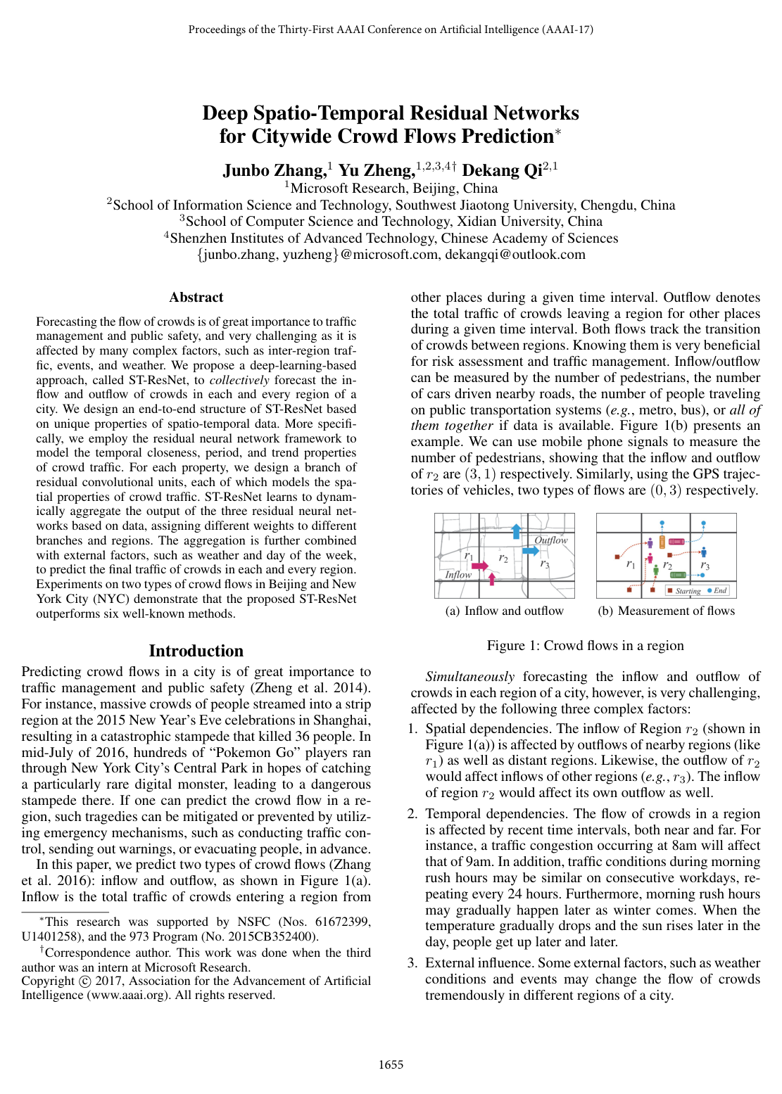
where $|\cdot|$ denotes set cardinality. Inflow measures the aggregate count of transitions entering region $(i, j)$ from any external region, while outflow measures transitions exiting region $(i, j)$ to any external region during interval $t$ .

The combined inflow and outflow measurements across all $I \times J$ regions at time interval $t$ form a 3D observation tensor $X_t \in \mathbb{R}^{2 \times I \times J}$ , where $(X_t)_{0, i, j} = x_t^{in, i, j}$ and $(X_t)_{1, i, j} = x_t^{out, i, j}$ .
Knowl 6 — ST-ResNet Training Algorithm
algorithm
The training process for ST-ResNet constructs multi-scale temporal sequences and external factor representations from historical data, optimizing network parameters via backpropagation with the Adam optimizer.
Input: Historical flow observations: { $X_0, \dots, X_{n-1}$ }
       External feature vectors: { $E_0, \dots, E_{n-1}$ }
       Lengths of closeness, period, trend sequences: $l_c, l_p, l_q$
       Period length: $p$
       Trend span length: $q$
Output: Trained ST-ResNet model with parameters $\theta$
// Step 1: Construct training dataset
$D \leftarrow \emptyset$
for all available time intervals $t$ where $\max(l_c, l_p \cdot p, l_q \cdot q) \le t \le n - 1$ do
     $S_c \leftarrow [X_{t-l_c}, X_{t-(l_c-1)}, \dots, X_{t-1}]$
     $S_p \leftarrow [X_{t-l_p \cdot p}, X_{t-(l_p-1) \cdot p}, \dots, X_{t-p}]$
     $S_q \leftarrow [X_{t-l_q \cdot q}, X_{t-(l_q-1) \cdot q}, \dots, X_{t-q}]$
    Add training instance $(\{S_c, S_p, S_q, E_t\}, X_t)$ to $D$
end for
// Step 2: Model parameter optimization
Initialize all learnable parameters $\theta$ in ST-ResNet
repeat
    Randomly sample a mini-batch $D_b$ from $D$
    Compute prediction $\widehat{X}_t = \tanh(X_{Res} + X_{Ext})$ for each instance in $D_b$
    Compute loss $\mathcal{L}(\theta) = \|X_t - \widehat{X}_t\|_2^2$
    Update parameters $\theta$ using Adam to minimize $\mathcal{L}(\theta)$ over $D_b$
until stopping criterion is met
The training uses mean squared error (MSE) as the objective function $\mathcal{L}(\theta) = \|X_t - \widehat{X}_t\|_2^2$ on Min-Max scaled flow targets in $[-1, 1]$ . Early stopping is guided by validation set performance, after which the model is fine-tuned on the combined training and validation data.
Knowl 7 — External Factor Feature Extraction and Embedding
model/method
ST-ResNet incorporates external environmental factors that cause irregular variations in urban mobility into a feature vector $E_t$ at target time interval $t$ :
1. Categorical Features: Weather conditions (16 discrete categories, e.g., sunny, rainy), holiday indicators (binary flag), and day-of-week metadata (day index, weekday vs. weekend) are transformed into binary vectors via one-hot encoding.
2. Continuous Features: Meteorological measurements, including temperature (in $^\circ\text{C}$ ) and wind speed (in mph), are normalized to $[0, 1]$ using Min-Max scaling.
The concatenated external feature vector $E_t$ is fed into a two-layer fully connected (FC) neural network:
- The first FC layer acts as an embedding layer for each sub-factor followed by a non-linear activation function.
- The second FC layer maps the low-dimensional embedding to a tensor $X_{Ext} \in \mathbb{R}^{2 \times I \times J}$ matching the spatial dimensions of the crowd flow grid.
When forecasting for a future interval $t$ where actual weather is unavailable, weather forecasts for time interval $t$ or measurements from interval $t-1$ are used.

Knowl 8 — Empirical Evaluation and Ablation on Beijing Taxi Flow Prediction

data/table

The performance of ST-ResNet was evaluated on the TaxiBJ dataset (taxicab GPS trajectories in Beijing spanning four intervals between 2013 and 2016, with a $32 \times 32$ grid and 30-minute time intervals). Models were evaluated using Root Mean Square Error (RMSE) against ground truth flow values:

Model	Description	RMSE
HA	Historical Average	57.69
ARIMA	Auto-Regressive Integrated Moving Average	22.78
SARIMA	Seasonal ARIMA	26.88
VAR	Vector Auto-Regressive	22.88
ST-ANN	Spatio-Temporal Artificial Neural Network	19.57
DeepST	Deep Spatio-Temporal Baseline	18.18
ST-ResNet Variants
L2-E	2 residual units + External factors	17.67
L4-E	4 residual units + External factors	17.51
L12-E	12 residual units + External factors	16.89
L12-E-BN	12 residual units + External factors + Batch Normalization	16.69
L12-single-E	12 units (1 conv per unit) + External factors	17.40
L12	12 residual units (without external factors)	17.00
L12-E-noFusion	12 residual units + External (simple sum, no parametric fusion)	17.96

Key empirical findings from the ablation study:

Depth scaling: Increasing the number of residual units from 2 to 12 progressively reduces RMSE ( $17.67 \to 17.51 \to 16.89$ ), confirming that deeper networks capture broader spatial dependencies.
Batch Normalization: Adding BN before ReLU activations inside the residual units yields the top performance (RMSE 16.69).
External Factors: Including external features improves RMSE over the baseline structure ( $16.89$ vs. $17.00$ ).
Parametric-Matrix Fusion: Replacing parametric-matrix-based fusion with simple addition ( $X_c + X_p + X_q$ ) worsens RMSE from 16.89 to 17.96, demonstrating that spatial weighting across temporal branches is critical.

Knowl 9 — Empirical Evaluation on New York City Bike Flow Prediction

data/table

ST-ResNet was evaluated on the BikeNYC dataset (Citi Bike trip trajectories from April 1 to September 30, 2014, partitioned into a $16 \times 8$ grid at 1-hour time intervals to predict station pickup new-flows and drop-off end-flows). A 4-residual-unit ST-ResNet was compared against classical and deep learning baselines using Root Mean Square Error (RMSE):

ST-ResNet achieves an RMSE of 6.33, outperforming the previous state-of-the-art DeepST-CPTM (7.43) by a 14.8% relative error reduction, and outperforming classical statistical baselines (ARIMA, SARIMA, VAR) by up to 37.1% relative reduction.

Coverage note — None was omitted; all primary architectural components, mathematical formulations, training procedures, external feature representations, and empirical benchmark results on TaxiBJ and BikeNYC have been captured.

References

1.Abadi, A.; Rajabioun, T.; and Ioannou, P. A. 2015. Traffic flow prediction for road transportation networks with limited traffic data. IEEE Transactions on Intelligent Transportation Systems 16(2):653–662.
2.Chollet, F. 2015. Keras. https://github.com/fchollet/keras.
3.Fan, Z.; Song, X.; Shibasaki, R.; and Adachi, R. 2015. Citymomentum: an online approach for crowd behavior prediction at a citywide level. In ACM UbiComp, 559–569. ACM.
4.He, K.; Zhang, X.; Ren, S.; and Sun, J. 2015. Deep residual learning for image recognition. In IEEE CVPR.
5.He, K.; Zhang, X.; Ren, S.; and Sun, J. 2016. Identity mappings in deep residual networks. In ECCV.
6.Hoang, M. X.; Zheng, Y.; and Singh, A. K. 2016. Forecasting citywide crowd flows based on big data. In ACM SIGSPATIAL.
7.Ioffe, S., and Szegedy, C. 2015. Batch normalization: Accelerating deep network training by reducing internal covariate shift. In ICML, 448–456.
8.Jain, V.; Murray, J. F.; Roth, F.; Turaga, S.; Zhigulin, V.; Briggman, K. L.; Helmstaedter, M. N.; Denk, W.; and Seung, H. S. 2007. Supervised learning of image restoration with convolutional networks. In ICCV, 1–8. IEEE.
9.Kingma, D., and Ba, J. 2014. Adam: A method for stochastic optimization. arXiv preprint arXiv:1412.6980.
10.Krizhevsky, A.; Sutskever, I.; and Hinton, G. E. 2012. ImageNet classification with deep convolutional neural networks. In NIPS.
11.LeCun, Y.; Bottou, L.; Bengio, Y.; and Haffner, P. 1998. Gradient-based learning applied to document recognition. Proceedings of the IEEE 86(11):2278–2324.
12.LeCun, Y. A.; Bottou, L.; Orr, G. B.; and Müller, K.-R. 2012. Efficient backprop. In Neural networks: Tricks of the trade. Springer.
13.Li, Y.; Zheng, Y.; Zhang, H.; and Chen, L. 2015. Traffic prediction in a bike-sharing system. In ACM SIGSPATIAL.
14.Long, J.; Shelhamer, E.; and Darrell, T. 2015. Fully convolutional networks for semantic segmentation. In IEEE CVPR, 3431–3440.
15.Mathieu, M.; Couprie, C.; and LeCun, Y. 2015. Deep multi-scale video prediction beyond mean square error. arXiv preprint arXiv:1511.05440.
16.Nair, V., and Hinton, G. E. 2010. Rectified linear units improve restricted boltzmann machines. In ICML, 807–814.
17.Silva, R.; Kang, S. M.; and Airoldi, E. M. 2015. Predicting traffic volumes and estimating the effects of shocks in massive transportation systems. Proceedings of the National Academy of Sciences 112(18):5643–5648.
18.Song, X.; Zhang, Q.; Sekimoto, Y.; and Shibasaki, R. 2014. Prediction of human emergency behavior and their mobility following large-scale disaster. In ACM SIGKDD, 5–14. ACM.
19.Sutskever, I.; Vinyals, O.; and Le, Q. V. 2014. Sequence to sequence learning with neural networks. In NIPS, 3104–3112.
20.Theano Development Team. 2016. Theano: A Python framework for fast computation of mathematical expressions. arXiv e-prints abs/1605.02688.
21.Xingjian, S.; Chen, Z.; Wang, H.; Yeung, D.-Y.; Wong, W.-k.; and WOO, W.-c. 2015. Convolutional lstm network: A machine learning approach for precipitation nowcasting. In NIPS, 802–810.
22.Xu, Y.; Kong, Q.-J.; Klette, R.; and Liu, Y. 2014. Accurate and interpretable bayesian mars for traffic flow prediction. IEEE Transactions on Intelligent Transportation Systems 15(6):2457–2469.
23.Zhang, J.; Zheng, Y.; Qi, D.; Li, R.; and Yi, X. 2016. DNN-based prediction model for spatial-temporal data. In ACM SIGSPATIAL.
24.Zheng, Y.; Capra, L.; Wolfson, O.; and Yang, H. 2014. Urban computing: concepts, methodologies, and applications. ACM Transactions on Intelligent Systems and Technology (TIST) 5(3):38.
25.Zheng, Y. 2015. Methodologies for cross-domain data fusion: An overview. IEEE transactions on big data 1(1):16–34.

Citation

MLA

Zhang, J., et al. “Deep Spatio-Temporal Residual Networks for Citywide Crowd Flows Prediction”. Proceedings of the AAAI Conference on Artificial Intelligence, vol. 31, no. 1, 2017, https://doi.org/10.1609/aaai.v31i1.10735.

APA

Zhang, J., Zheng, Y., & Qi, D. (2017). Deep Spatio-Temporal Residual Networks for Citywide Crowd Flows Prediction. Proceedings of the AAAI Conference on Artificial Intelligence, 31(1). https://doi.org/10.1609/aaai.v31i1.10735

Chicago

Zhang, J., Y. Zheng, and D. Qi. 2017. “Deep Spatio-Temporal Residual Networks for Citywide Crowd Flows Prediction”. Proceedings of the AAAI Conference on Artificial Intelligence 31 (1). https://doi.org/10.1609/aaai.v31i1.10735.

Harvard

Zhang, J., Zheng, Y. and Qi, D. (2017) “Deep Spatio-Temporal Residual Networks for Citywide Crowd Flows Prediction”, Proceedings of the AAAI Conference on Artificial Intelligence, 31(1). Available at: https://doi.org/10.1609/aaai.v31i1.10735.

Vancouver

1. Zhang J, Zheng Y, Qi D (2017) Deep Spatio-Temporal Residual Networks for Citywide Crowd Flows Prediction. Proceedings of the AAAI Conference on Artificial Intelligence. https://doi.org/10.1609/aaai.v31i1.10735

BibTeX

@article{Zhang_2017, title={Deep Spatio-Temporal Residual Networks for Citywide Crowd Flows Prediction}, volume={31}, ISSN={2159-5399}, url={http://dx.doi.org/10.1609/aaai.v31i1.10735}, DOI={10.1609/aaai.v31i1.10735}, number={1}, journal={Proceedings of the AAAI Conference on Artificial Intelligence}, publisher={Association for the Advancement of Artificial Intelligence (AAAI)}, author={Zhang, Junbo and Zheng, Yu and Qi, Dekang}, year={2017}, month=Feb }

Metadata:Crossref

Source Code

This paper has an official code repository available. Click below to access the source code.

View Repository

Access the Paper

This paper is available from its original source. Click below to access the PDF.

Open PDF

Model	RMSE
ARIMA	10.07
SARIMA	10.56
VAR	9.92
DeepST-C	8.39
DeepST-CP	7.64
DeepST-CPT	7.56
DeepST-CPTM	7.43
ST-ResNet [ours, 4 residual units]	6.33

Deep Spatio-Temporal Residual Networks for Citywide Crowd Flows Prediction

Abstract

Topics

Keywords

Table of Contents

Knowls

Knowl 1 — ST-ResNet Architecture for Crowd Flow Prediction

Knowl 2 — Parametric-Matrix-Based Spatio-Temporal Fusion

Knowl 3 — Multi-Branch Temporal Sequence Partitioning

Knowl 4 — Residual Convolutional Unit Architecture for Spatio-Temporal Grids

Knowl 5 — Grid-Based Crowd Inflow and Outflow Formulation

Knowl 6 — ST-ResNet Training Algorithm