Beyond short snippets: Deep networks for video classification

Joe Yue-Hei NgMatthew HausknechtSudheendra VijayanarasimhanOriol VinyalsRajat MongaGeorge Toderici

article2015CVPR2,460 citations

Proposes convolutional temporal pooling and recurrent LSTM architectures that extend deep convolutional networks to full-length video classification, substantially outperforming prior methods on Sports-1M and UCF-101.

Listen

Automated video classification is a critical capability for organizing, searching, and moderating massive volumes of video content online. While deep convolutional neural networks excel at recognizing objects in static images, standard approaches struggle with video because they either process isolated still frames or focus narrowly on short snippets lasting only a few seconds. Treating video frames independently discards vital temporal context and confusing background elements, while processing high frame rates across long durations has historically been too computationally expensive.

The article evaluates whether aggregating visual information across entire videosspanning up to several minutescan significantly improve classification accuracy while maintaining manageable computational demands.

To address this, the researchers evaluated two main model designs using parameter sharing to keep network size constant regardless of video length: convolutional temporal feature pooling architectures (combining frame-level features across time) and recurrent neural networks using Long Short-Term Memory cells (explicitly tracking temporal sequences across frames). The models were tested on the large-scale Sports-1M dataset (1.1 million videos) and the benchmark UCF-101 action dataset (13,320 videos). To manage computational load, networks processed low-rate video frames (such as 1 frame per second) supplemented with optical flow motion images to capture fast movement.

The study established several key findings. First, incorporating longer temporal context substantially boosted accuracy, with the top-performing models achieving a video-level top-1 accuracy of 73.1% on Sports-1M compared to the previous state-of-the-art of 60.9%—a relative gain of 20%. Second, on UCF-101, the architectures reached 88.6% accuracy, surpassing prior approaches. Third, max-pooling over the final convolutional layer outperformed pooling after fully connected layers, demonstrating the necessity of preserving spatial information before aggregating across time. Fourth, explicit motion data through optical flow provided massive gains on clean, well-framed videos (improving UCF-101 accuracy from 82.6% to 88.2%), and when paired with Long Short-Term Memory models, it provided measurable improvements even on noisy, unconstrained real-world videos where basic pooling failed to benefit.

These results demonstrate that capturing extended temporal evolution is essential for high-performance video analysis. Deploying these architectures enables significantly more accurate content categorization and automated moderation on diverse web videos. Furthermore, the findings show that organizations can achieve state-of-the-art video understanding without processing every single frame, effectively controlling operational and computational infrastructure costs through low frame-rate sampling combined with motion features.

Organizations implementing automated video recognition systems should prioritize architectures that pool features across full videos rather than relying on short-clip analyses. For clean, well-segmented datasets, standard convolutional pooling combined with optical flow provides high performance with lower complexity; for noisy, real-world video platforms, deploying recurrent Long Short-Term Memory models is recommended to effectively leverage motion cues. As a next step, research and engineering teams should investigate deeper temporal integration within the lower convolutional layers, such as recurrent convolutional networks, to improve feature extraction directly from video streams.

Confidence in these findings is high across both large-scale and controlled benchmarks. However, stakeholders should note that the quality and nature of the video source heavily influence performance: benefits from motion features diminish when camera work is erratic or video resolution is poor unless paired with advanced sequential modeling.

arXiv: 1503.08909
Cover for Beyond short snippets: Deep networks for video classification

Abstract

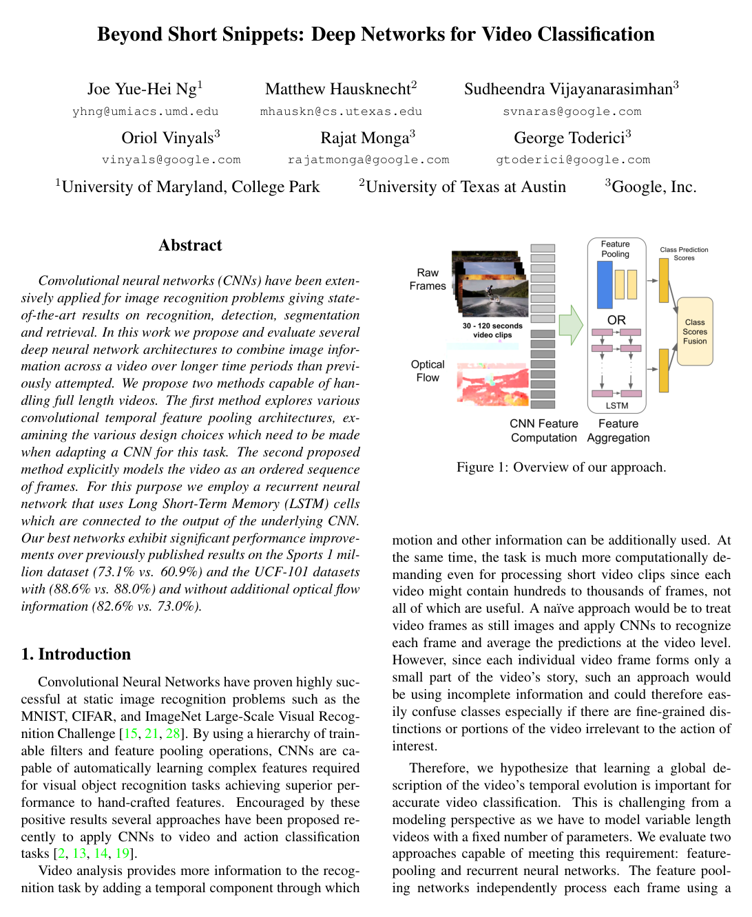
Convolutional neural networks (CNNs) have been extensively applied for image recognition problems giving state-of-the-art results on recognition, detection, segmentation and retrieval. In this work we propose and evaluate several deep neural network architectures to combine image information across a video over longer time periods than previously attempted. We propose two methods capable of handling full length videos. The first method explores various convolutional temporal feature pooling architectures, examining the various design choices which need to be made when adapting a CNN for this task. The second proposed method explicitly models the video as an ordered sequence of frames. For this purpose we employ a recurrent neural network that uses Long Short-Term Memory (LSTM) cells which are connected to the output of the underlying CNN. Our best networks exhibit significant performance improvements over previously published results on the Sports 1 million dataset (73.1% vs. 60.9%) and the UCF-101 datasets with (88.6% vs. 88.0%) and without additional optical flow information (82.6% vs. 72.8%).

Table of Contents

  • 1 Introduction
  • 2 Related Work
  • 3 Approach
  • 3.1 Feature Pooling Architectures
  • 3.2 LSTM Architecture
  • 3.3 Training and Inference
  • 3.4 Optical Flow
  • 4 Results
  • 4.1 Sports-1M dataset
  • 4.2 UCF-101 Dataset
  • 5 Conclusion
  • References

Knowls

  1. Knowl 1 — Deep Video LSTM Architecture for Long-Sequence Temporal Modeling

    model/method

    To model video as an ordered sequence of frames over extended time periods, a deep recurrent neural network composed of five stacked Long Short-Term Memory (LSTM) layers is connected to the feature activations produced by an underlying frame-level Convolutional Neural Network (CNN, such as GoogLeNet or AlexNet). Each LSTM layer contains 512 memory cells. Given a sequence of frame feature vectors x=(x1,,xT)x = (x_1, \dots, x_T) across time steps t=1,,Tt = 1, \dots, T, each LSTM cell computes an input gate iti_t, forget gate ftf_t, cell state ctc_t, output gate oto_t, and hidden state vector hth_t according to:

    it=σ(Wxixt+Whiht1+Wcict1+bi)i_t = \sigma(W_{xi} x_t + W_{hi} h_{t-1} + W_{ci} c_{t-1} + b_i)

    ft=σ(Wxfxt+Whfht1+Wcfct1+bf)f_t = \sigma(W_{xf} x_t + W_{hf} h_{t-1} + W_{cf} c_{t-1} + b_f)

    ct=ftct1+ittanh(Wxcxt+Whcht1+bc)c_t = f_t c_{t-1} + i_t \tanh(W_{xc} x_t + W_{hc} h_{t-1} + b_c)

    ot=σ(Wxoxt+Whoht1+Wcoct+bo)o_t = \sigma(W_{xo} x_t + W_{ho} h_{t-1} + W_{co} c_t + b_o)

    ht=ottanh(ct)h_t = o_t \tanh(c_t)

    where σ(z)=11+ez\sigma(z) = \frac{1}{1 + e^{-z}} denotes the logistic sigmoid activation function, WW terms denote weight matrices, and bb terms denote bias vectors, with all parameters shared across time steps tt. A softmax classification layer produces a class prediction at each time step based on the hidden state of the top LSTM layer. To generate a single video-level prediction at inference, predictions across all time steps are linearly weighted by gt=t/Tg_t = t / T, summed, and the argmax class is returned.

  2. Knowl 2 — Temporal Feature Pooling Architectures for Video CNNs

    model/method

    Five distinct architectural designs aggregate frame-level CNN representations across an unordered set of TT video frames using max-pooling operations (which produce sparser gradient updates and faster convergence than average pooling or fully connected pooling):

    1. Conv Pooling: Temporal max-pooling is applied element-wise across all TT frames directly on the activations of the final convolutional layer. This preserves the 2D spatial arrangement of features across time before feeding the pooled features into the network's fully connected layers.

    2. Late Pooling: Each frame's convolutional features are first passed independently through two fully connected layers with shared parameters. Temporal max-pooling is then applied across frames on the final fully connected layer outputs prior to softmax classification.

    3. Slow Pooling: A two-stage hierarchical pooling structure. First, 1D temporal max-pooling is applied locally across 10-frame windows of convolutional features with a stride of 5 frames. Each local pooled output is processed by shared fully connected layers. In the second stage, a global temporal max-pooling layer aggregates the outputs of all fully connected towers.

    4. Local Pooling: Applies a single stage of local temporal max-pooling over 10-frame windows of convolutional features, passes the pooled representations through shared fully connected layers, and connects the concatenated outputs directly to a single wide softmax classifier without a second pooling stage.

    5. Time-Domain Convolution: Inserts a 1D temporal convolutional layer consisting of 256 kernels of size 3×33 \times 3 across 10 frames with a frame stride of 5 on top of the last convolutional layer. Temporal max-pooling is subsequently performed across time on these temporal-convolutional features.

  3. Knowl 3 — Linearly Weighted Frame Backpropagation for Video LSTM Training

    algorithm

    To train a multi-frame video LSTM while prioritizing predictions after the model's internal memory state has accumulated sufficient temporal context, backpropagation is performed at every frame time step with a time-dependent gradient scaling factor gtg_t.

    Input: Video frame sequence X=(x1,x2,,xT)X = (x_1, x_2, \dots, x_T), video ground truth label yy
    Output: Updated parameter weights Θ\Theta for the CNN and stacked LSTM network
    Initialize hidden and cell states: h0(l)=0,c0(l)=0h_0^{(l)} = 0, c_0^{(l)} = 0 for all layers l{1,,5}l \in \{1, \dots, 5\}
    for t=1t = 1 to TT do
        Extract CNN feature vector ft=CNN(xt)f_t = \text{CNN}(x_t)
        Forward propagate ftf_t through stacked LSTM layers to compute ht(5)h_t^{(5)}
        Compute class probability distribution y^t=Softmax(FC(ht(5)))\hat{y}_t = \text{Softmax}(\text{FC}(h_t^{(5)}))
        Compute frame cross-entropy loss Lt=logy^t,yL_t = -\log \hat{y}_{t, y}
        Compute gradient gain weight gt=t/Tg_t = t / T
        Scale frame loss: L~t=gtLt\tilde{L}_t = g_t \cdot L_t
        Backpropagate L~t\tilde{L}_t through LSTM layers and fine-tune underlying CNN layers
    end for
    Apply parameter update using Downpour SGD with momentum 0.9 and weight decay 5×1045 \times 10^{-4}
  4. Knowl 4 — Progressive Multi-Frame Network Expansion Strategy

    model/method

    To reduce the computational burden of training multi-frame temporal feature pooling networks from scratch on long video clips (e.g., 120 frames), a staged network expansion strategy is employed. Because temporal max-pooling models utilize convolutional towers whose parameters are shared across all frames, parameter configurations between 1-frame, 30-frame, and 120-frame networks are structurally identical except for the temporal pooling dimension.

    The network is first initialized from image models pre-trained on ImageNet and trained as a single-frame model on the target video dataset. The learned single-frame weights are then transferred to initialize a 30-frame pooling model. After fine-tuning the 30-frame network, its weights are transferred to initialize a 120-frame network for final fine-tuning. This progressive transfer drastically accelerates convergence compared to training long-sequence networks directly from scratch.

  5. Knowl 5 — Optical Flow Preprocessing and Image-to-Flow Weight Initialization

    model/method

    To incorporate explicit apparent motion into models sampling frames at low rates (such as 1 fps), optical flow is extracted from adjacent video frames sampled at 15 fps using the TV-L1L_1 algorithm. The horizontal (uu) and vertical (vv) displacement fields are thresholded within [40,40][-40, 40] pixels and rescaled linearly to [0,255][0, 255]. A three-channel pseudo-image is constructed by assigning uu to the first channel, vv to the second channel, and setting the third channel to 0.

    When training CNNs on optical flow images, initializing network weights from models pre-trained on raw RGB image frames achieves significantly faster training convergence and higher accuracy than training from scratch. This occurs because low-level spatial visual primitives (such as edge and boundary filters) learned on static images transfer effectively to detecting motion boundaries in optical flow fields.

  6. Knowl 6 — Performance Comparison of Temporal Feature Pooling Architectures on Sports-1M

    data/table

    Evaluation of five feature-pooling variations on the Sports-1M dataset using a 120-frame AlexNet architecture sampled at 1 fps demonstrates that max-pooling over the final convolutional layer (Conv Pooling) outperforms pooling at fully connected stages or using 1D time-domain convolutions, confirming the importance of preserving 2D spatial layouts across the time domain.

    Method Clip Hit@1 (%) Video Hit@1 (%) Video Hit@5 (%)
    Conv Pooling 68.7 71.1 89.3
    Local Pooling 68.1 70.4 88.9
    Slow Pooling 67.1 69.7 88.4
    Late Pooling 65.1 67.5 87.2
    Time-Domain Convolution 64.2 67.2 87.2
  7. Knowl 7 — Large-Scale Video Classification Benchmark on Sports-1M

    data/table

    Performance of long-temporal-context models on the 1.1 million video Sports-1M dataset (487 sports categories) compared with prior state-of-the-art 3D-convolution methods (Slow Fusion). Hit@kk measures the fraction of test videos where at least one ground-truth label appears in the top kk predictions. Both Conv Pooling (120 frames) and Deep LSTM (30 frames) with GoogLeNet backbones combined with optical flow establish new state-of-the-art results, yielding an absolute improvement of over 12% in video Hit@1 compared to prior short-clip methods.

    Category Method Frames Clip Hit@1 (%) Hit@1 (%) Hit@5 (%)
    Prior Results Single Frame Baseline 1 41.1 59.3 77.7
    Prior Results Slow Fusion CNN 15 41.9 60.9 80.2
    This Paper Conv Pooling (RGB + Flow) 120 70.8 72.4 90.8
    This Paper LSTM (RGB + Flow) 30 N/A 73.1 90.5
  8. Knowl 8 — Action Classification Accuracy on the UCF-101 Benchmark

    data/table

    Evaluation on the UCF-101 dataset (101 action classes, 13,320 videos) averaged over the standard 3-fold train/test splits. Networks pre-trained on Sports-1M and fine-tuned on UCF-101 outperform prior hand-crafted feature methods (Improved Dense Trajectories) and two-stream CNN baselines. The 30-frame unrolled LSTM combining RGB frames and optical flow achieves the highest overall accuracy.

    Method 3-fold Accuracy (%)
    Improved Dense Trajectories (IDTF) 87.9
    Slow Fusion CNN 65.4
    Single Frame CNN Model (Images) 73.0
    Single Frame CNN Model (Optical Flow) 73.9
    Two-Stream CNN (Flow + RGB Averaging) 86.9
    Two-Stream CNN (Flow + RGB SVM Fusion) 88.0
    Single Frame Baseline 73.3
    Conv Pooling of Image Frames + Flow (30 Frames) 87.6
    Conv Pooling of Image Frames + Flow (120 Frames) 88.2
    LSTM with 30 Frame Unroll (Flow + RGB Frames) 88.6
  9. Knowl 9 — Robustness of LSTMs vs Feature Pooling to Noisy Optical Flow

    empirical result

    On curated, well-trimmed datasets such as UCF-101, optical flow features provide a dramatic boost in video classification accuracy (improving performance from 82.6% for raw frames to 88.2%–88.6% when fused with optical flow). In contrast, on unconstrained web videos (such as Sports-1M) where camera motion and editing cuts introduce high levels of noise into optical flow fields, an optical flow model alone achieves only 59.7% Hit@1 (compared to 72.1% for raw RGB frames).

    In this noisy setting, late fusion of optical flow with temporal Conv Pooling provides no meaningful improvement over raw frames alone (71.7% to 71.8% Hit@1). However, when optical flow is processed using an LSTM network, the recurrent architecture is able to integrate noisy motion cues over time, improving classification performance from 72.1% (RGB only) to 73.1% Hit@1 (RGB + Optical Flow).

  10. Knowl 10 — Impact of Frame Sampling Rate and Temporal Coverage on Classification

    empirical result

    On the UCF-101 dataset (where videos average 10–15 seconds in duration), reducing the frame sampling rate from 30 fps to 6 fps for a 30-frame Conv Pooling model increases 3-fold classification accuracy from 80.8% (1 second of total context) to 82.0% (5 seconds of total context). When expanding the input budget to 120 frames (covering 4 seconds at 30 fps and 20 seconds at 6 fps), both frame rates achieve an identical 82.6% accuracy.

    Further reducing the sampling rate to 1 fps yields no additional performance gain. This demonstrates that expanding the total temporal duration covered by the frame budget is critical up to the point where the global context of the video is captured, after which lowering the sampling rate produces diminishing returns.

Coverage note — None was omitted; all key architectural variations, LSTM mathematical formulations, training algorithms, optical flow representations, and benchmark results on Sports-1M and UCF-101 are covered.

References

  1. 1.M. Baccouche, F. Mamalet, C. Wolf, C. Garcia, and A. Baskurt. Action classification in soccer videos with long short-term memory recurrent neural networks. In Proc. ICANN, pages 154–159, Thessaloniki, Greece, 2010. 2
  2. 2.M. Baccouche, F. Mamalet, C. Wolf, C. Garcia, and A. Baskurt. Sequential Deep Learning for Human Action Recognition. In 2nd International Workshop on Human Behavior Understanding (HBU), pages 29–39, Nov. 2011. 1, 2
  3. 3.Y. Bengio, P. Simard, and P. Frasconi. Learning long-term dependencies with gradient descent is difficult. IEEE Trans. on Neural Networks, 5(2):157–166, 1994. 2
  4. 4.Y.-L. Boureau, J. Ponce, and Y. Lecun. A theoretical analysis of feature pooling in visual recognition. In Proc. ICML, pages 111–118, Haifa, Israel, 2010. 3
  5. 5.S. Fernandez, A. Graves, and J. Schmidhuber. Phoneme ´ recognition in TIMIT with BLSTM-CTC. CoRR, abs/0804.3269, 2008. 2
  6. 6.F. A. Gers, N. N. Schraudolph, and J. Schmidhuber. Learning precise timing with LSTM recurrent networks. JMLR, 3:115–143, 2002. 4
  7. 7.A. Graves and N. Jaitly. Towards end-to-end speech recognition with recurrent neural networks. In Proc. ICML, pages 1764–1772, Beijing, China, 2014. 2
  8. 8.A. Graves, M. Liwicki, S. Fernandez, R. Bertolami, H. Bunke, and J. Schmidhuber. A novel connectionist system for unconstrained handwriting recognition. IEEE Trans. PAMI, 31(5):855–868, 2009. 2
  9. 9.A. Graves, A.-R. Mohamed, and G. E. Hinton. Speech recognition with deep recurrent neural networks. CoRR, abs/1303.5778, 2013. 2, 4
  10. 10.A. Graves and J. Schmidhuber. Offline handwriting recognition with multidimensional recurrent neural networks. In Proc. NIPS, pages 545–552, Vancouver, B.C., Canada, 2008. 2
  11. 11.S. Hochreiter and J. Schmidhuber. Long short-term memory. Neural Computing, 9(8):1735–1780, Nov. 1997. 2
  12. 12.M. Jain, H. Jegou, and P. Bouthemy. Better exploiting mo- ´ tion for better action recognition. In Proc. CVPR, pages 2555–2562, Portland, Oregon, USA, 2013. 2, 3
  13. 13.S. Ji, W. Xu, M. Yang, and K. Yu. 3D convolutional neural networks for human action recognition. IEEE Trans. PAMI, 35(1):221–231, Jan. 2013. 1, 2
  14. 14.A. Karpathy, G. Toderici, S. Shetty, T. Leung, R. Sukthankar, and L. Fei-Fei. Large-scale video classification with convolutional neural networks. In Proc. CVPR, pages 1725–1732, Columbus, Ohio, USA, 2014. 1, 2, 6, 7, 8
  15. 15.A. Krizhevsky, I. Sutskever, and G. E. Hinton. ImageNet classification with deep convolutional neural networks. In Proc. NIPS, pages 1097–1105, Lake Tahoe, Nevada, USA, 2012. 1, 2, 3
  16. 16.H. Kuehne, H. Jhuang, E. Garrote, T. Poggio, and T. Serre. HMDB: a large video database for human motion recognition. In Proc. ICCV, pages 2556–2563, Barcelona, Spain, 2011. 2
  17. 17.I. Laptev, M. Marszaek, C. Schmid, and B. Rozenfeld. Learning realistic human actions from movies. In Proc. CVPR, pages 1–8, Anchorage, Alaska, USA, 2008. 2, 3
  18. 18.S. Reiter, B. Schuller, and G. Rigoll. A combined LSTM-RNN - HMM - approach for meeting event segmentation and recognition. In Proc. ICASSP, pages 393–396, Toulouse, France, 2006. 2
  19. 19.K. Simonyan and A. Zisserman. Two-stream convolutional networks for action recognition in videos. In Proc. NIPS, pages 568–576, Montreal, Canada, 2014. 1, 2, 5, 8
  20. 20.K. Soomro, A. R. Zamir, and M. Shah. UCF101: A dataset of 101 human actions classes from videos in the wild. In CRCV-TR-12-01, 2012. 7
  21. 21.C. Szegedy, W. Liu, Y. Jia, P. Sermanet, S. Reed, D. Anguelov, D. Erhan, V. Vanhoucke, and A. Rabinovich. Going deeper with convolutions. CoRR, abs/1409.4842, 2014. 1, 3, 4
  22. 22.H. Wang, A. Klaser, C. Schmid, and C.-L. Liu. Action recognition by dense trajectories. In Proc. CVPR, pages 3169–3176, Washington, DC, USA, 2011. 2
  23. 23.H. Wang and C. Schmid. Action Recognition with Improved Trajectories. In Proc. ICCV, pages 3551–3558, Sydney, Australia, 2013. 2, 5, 8
  24. 24.H. Wang, M. M. Ullah, A. Klser, I. Laptev, and C. Schmid. Evaluation of local spatio-temporal features for action recognition. In Proc. BMVC, pages 1–11, 2009. 2, 3
  25. 25.M. Wllmer, M. Kaiser, F. Eyben, B. Schuller, and G. Rigoll. LSTM-modeling of continuous emotions in an audiovisual affect recognition framework. Image Vision Computing, 31(2):153–163, 2013. 2
  26. 26.C. Zach, T. Pock, and H. Bischof. A duality based approach for realtime tv-l1 optical flow. In Proceedings of the 29th DAGM Conference on Pattern Recognition, pages 214–223, Berlin, Heidelberg, 2007. Springer-Verlag. 5
  27. 27.W. Zaremba and I. Sutskever. Learning to execute. CoRR, abs/1410.4615, 2014. 2
  28. 28.M. D. Zeiler and R. Fergus. Visualizing and understanding convolutional networks. In Proc. ECCV, pages 818–833, Zurich, Switzerland, 2014. 1, 3

Citation

MLA
Ng, J. Y.-H., et al. “Beyond Short Snippets: Deep Networks for Video Classification”. arXiv, 2015, http://arxiv.org/abs/1503.08909v2.
APA
Ng, J. Y.-H., Hausknecht, M., Vijayanarasimhan, S., Vinyals, O., Monga, R., & Toderici, G. (2015). Beyond Short Snippets: Deep Networks for Video Classification. arXiv. http://arxiv.org/abs/1503.08909v2
Chicago
Ng, J. Y.-H., M. Hausknecht, S. Vijayanarasimhan, O. Vinyals, R. Monga, and G. Toderici. 2015. “Beyond Short Snippets: Deep Networks for Video Classification”. arXiv. http://arxiv.org/abs/1503.08909v2.
Harvard
Ng, J.Y.-H. et al. (2015) “Beyond Short Snippets: Deep Networks for Video Classification”, arXiv [Preprint]. Available at: http://arxiv.org/abs/1503.08909v2.
Vancouver
1. Ng JY-H, Hausknecht M, Vijayanarasimhan S, Vinyals O, Monga R, Toderici G (2015) Beyond Short Snippets: Deep Networks for Video Classification. arXiv

BibTeX

@article{ng2015beyond,
  title = {Beyond Short Snippets: Deep Networks for Video Classification},
  author = {Ng, Joe Yue-Hei and Hausknecht, Matthew and Vijayanarasimhan, Sudheendra and Vinyals, Oriol and Monga, Rajat and Toderici, George},
  year = {2015},
  journal = {arXiv},
  url = {http://arxiv.org/abs/1503.08909v2},
  eprint = {1503.08909}
}
Metadata:arXiv

Access the Paper

This paper is available from its original source. Click below to access the PDF.

Open PDF

License: IEEE