Lower Bounds and Accelerated Algorithms for Bilevel Optimization

Kaiyi JiYingbin Liang

article2023JMLR66 citations

Establishes fundamental computational lower complexity bounds for bilevel optimization and presents AccBiO, an accelerated algorithm that achieves near-optimal convergence rates without requiring common gradient boundedness assumptions.

Listen

Bilevel optimization—a mathematical framework where one optimization problem is nested inside another—is central to high-impact machine learning applications such as hyperparameter tuning, meta-learning, and neural architecture search. Despite widespread adoption, the theoretical limits of bilevel optimization have remained poorly understood. Prior convergence analyses relied on restrictive technical assumptions, exhibited highly pessimistic execution times, and left open whether bilevel optimization is fundamentally harder to solve than simpler minimax problems.

The article establishes the theoretical performance limits of bilevel optimization and designs accelerated algorithms that push execution speeds toward these limits across two standard problem classes: strongly convex and convex settings with strongly convex inner objectives.

To establish computational limits, the article constructs worst-case problem instances and tracks how decision variables evolve across iterations. It also proposes an accelerated optimizer named AccBiO, which uses accelerated gradient steps for the inner problem, a heavy-ball method to solve linear subproblems, and momentum acceleration on outer-level updates. Numerical simulations on benchmark problems evaluate the runtime performance of AccBiO against existing standard bilevel algorithms.

The key findings are as follows. First, the article proves the first theoretical lower complexity bounds for bilevel optimization, showing that bilevel problems are fundamentally more difficult than minimax optimization. Second, AccBiO is the first accelerated algorithm proven to converge without requiring the assumption that outer-level gradients remain bounded. Third, for problems where the inner objective is quadratic, AccBiO matches the theoretical lower bounds up to logarithmic factors, achieving near-optimal complexity. Fourth, when outer-level gradients are bounded, the proposed approach significantly improves upper complexity bounds over existing algorithms.

These findings provide definitive benchmarks for computational efficiency and confirm that the structural differences between inner and outer levels make bilevel optimization strictly more demanding than minimax problems. In practical settings, deploying AccBiO offers significant reductions in computational runtime and memory usage for training complex machine learning models.

Organizations developing machine learning pipelines should adopt accelerated bilevel schemes like AccBiO for nested optimization tasks to achieve faster convergence. For further development, researchers should focus on closing the remaining theoretical gap for general inner objectives and extending these acceleration methods to non-convex problem landscapes, such as deep neural networks.

The findings are derived under the assumption that the inner-level problem is strongly convex with unique solutions, alongside Lipschitz continuous derivatives. For settings where the inner objective has multiple solutions or the overall landscape is non-convex, caution is warranted, as additional regularization or bounded domain projections may be necessary.

The Ohio State University University at Buffalo condition numbers machine learning numerical experiments bilevel optimization lower complexity bounds accelerated algorithms

arXiv: 2102.03926

Paper: Will Bilevel Optimizers Benefit from Loops, Kaiyi Ji et al. (2022). It provides foundational computational complexity bounds and error analyses for loop-based bilevel optimizer families (AID-BiO and ITD-BiO) that the source builds upon when establishing lower bounds and accelerated algorithms.
Paper: A Fully Single Loop Algorithm for Bilevel Optimization without Hessian Inverse, Junyi Li et al. (2022). It introduces a fully single-loop framework for hyper-gradient approximation in bilevel optimization without explicit Hessian inversion, providing direct background for the accelerated subproblem solvers analyzed in the source.
Paper: BOME! Bilevel Optimization Made Easy: A Simple First-Order Approach, Bo Liu et al. (2022). It details alternative first-order approaches and value-function reformulations for bilevel optimization, framing the baseline complexity challenges addressed by the source's accelerated methods.
Book: Convex Optimization: Algorithms and Complexity, Sébastien Bubeck (2015). It establishes the core black-box oracle complexity framework and foundational upper and lower bounds for first-order convex optimization that the source adapts to nested bilevel settings.
Paper: Accelerated Zeroth-Order and First-Order Momentum Methods from Mini to Minimax Optimization, Feihu Huang et al. (2022). It analyzes accelerated momentum methods for minimax optimization, establishing the baseline complexity against which the source proves bilevel problems are strictly harder.
Paper: A Differential Equation for Modeling Nesterov's Accelerated Gradient Method: Theory and Insights, Weijie Su et al. (2014). It analyzes the continuous-time dynamics and momentum mechanics of Nesterov's accelerated gradient method, which underpins the accelerated inner and outer updates developed in AccBiO.

Paper: Nested Learning: The Illusion of Deep Learning Architectures, Ali Behrouz et al. (2025). It generalizes multi-level and nested optimization into a broader nested learning architecture for deep neural network components and memory systems.

Cover for Lower Bounds and Accelerated Algorithms for Bilevel Optimization

Abstract

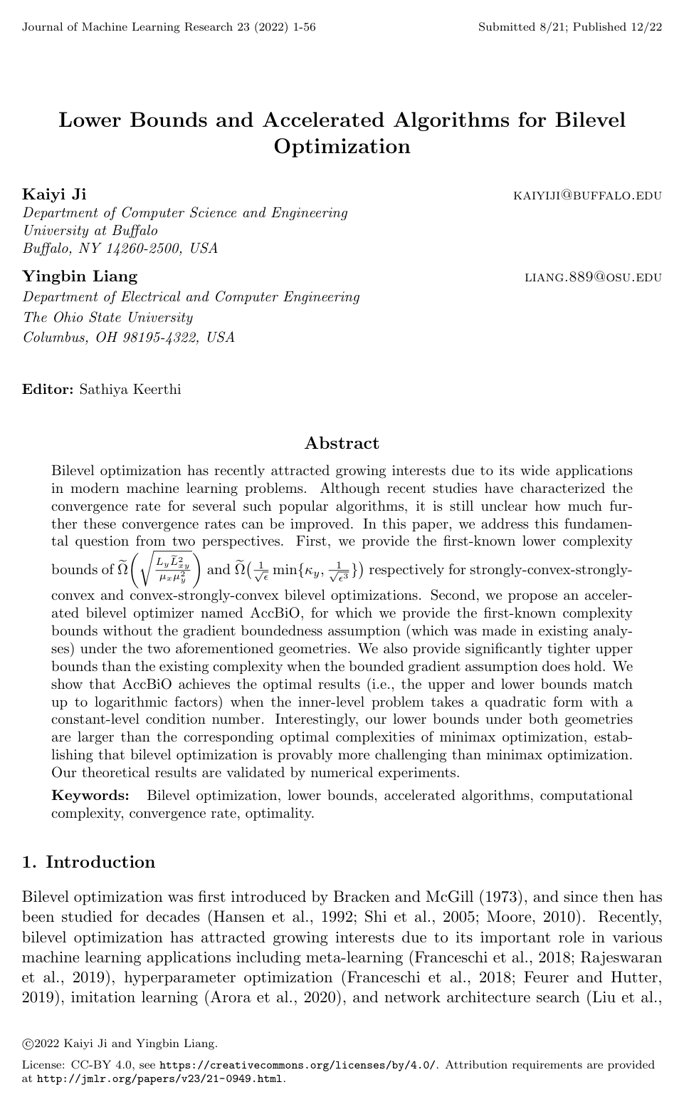
Bilevel optimization has recently attracted growing interests due to its wide applications in modern machine learning problems. Although recent studies have characterized the convergence rate for several such popular algorithms, it is still unclear how much further these convergence rates can be improved. In this paper, we address this fundamental question from two perspectives. First, we provide the first-known lower complexity bounds of \widetilde{\Omega}\left(\sqrt{\frac{L_y \bar{L}_{xy}^2}{\mu_x \mu_y^2}}\right) and \widetilde{\Omega}(\frac{1}{\sqrt{\epsilon}}\min{\kappa_y, \frac{1}{\sqrt{\epsilon^3}}}) respectively for strongly-convex-strongly-convex and convex-strongly-convex bilevel optimizations. Second, we propose an accelerated bilevel optimizer named AccBiO, for which we provide the first-known complexity bounds without the gradient boundedness assumption (which was made in existing analyses) under the two aforementioned geometries. We also provide significantly tighter upper bounds than the existing complexity when the bounded gradient assumption does hold. We show that AccBiO achieves the optimal results (i.e., the upper and lower bounds match up to logarithmic factors) when the inner-level problem takes a quadratic form with a constant-level condition number. Interestingly, our lower bounds under both geometries are larger than the corresponding optimal complexities of minimax optimization, establishing that bilevel optimization is provably more challenging than minimax optimization. Our theoretical results are validated by numerical experiments.

Topics

condition numbers machine learning numerical experiments optimization optimization problems quadratic form theoretical result numerical results

Keywords

bilevel optimization lower complexity bounds accelerated algorithms gradient-based hyperparameter optimization minimax optimization hypergradient-based algorithm linear bilevel programming convex bilevel optimization stochastic bilevel optimization

1. Introduction
1.1 Summary of Contributions
1.2 Related Works
2. Preliminaries on Bilevel Optimization
2.1 Bilevel Problem Class
2.2 Algorithm Class for Bilevel Optimization
2.3 Complexity Measures
3. Lower Bounds for Bilevel Optimization
3.1 Strongly-Convex-Strongly-Convex Bilevel Optimization
3.2 Convex-Strongly-Convex Bilevel Optimization
4. Accelerated Gradient Method and Upper Bounds for Bilevel Optimization
4.1 Accelerated Bilevel Optimization Algorithm: AccBiO
4.2 Strongly-Convex-Strongly-Convex Bilevel Optimization
4.3 Convex-Strongly-Convex Bilevel Optimization
4.4 Optimality of Bilevel Optimization and Discussion
5. Upper Bounds with Gradient Boundedness Assumption
5.1 Accelerated Bilevel Optimization Algorithm: AccBiO-BG
5.2 Strongly-Convex-Strongly-Convex Bilevel Optimization
5.3 Convex-Strongly-Convex Bilevel Optimization
6. Numerical Experiments
7. Conclusion and Discussion
Appendix
Appendix A. ITD-Based Bilevel Algorithms
Appendix B. Proof of Theorem 4
Appendix C. Proof of Theorem 6
Appendix D. Proof of Theorem 7
Appendix E. Proof of Theorem 8
Appendix F. Proof of Theorem 9
Appendix G. Proof of Theorem 10
Appendix H. Proof of Theorem 11
Appendix I. Proof of Theorem 12
Appendix J. Proof of Theorem 13
Appendix K. Proof of Theorem 14
References

Knowls

Knowl 1 — Lower Complexity Bound for Strongly-Convex-Strongly-Convex Bilevel Optimization
theoretical result
Consider the unconstrained bilevel optimization problem $\min_{x \in \mathbb{R}^p} \Phi(x) := f(x, y^*(x))$ subject to $y^*(x) = \arg\min_{y \in \mathbb{R}^q} g(x, y)$ , where $\Phi(x)$ is $\mu_x$ -strongly convex, $g(x, \cdot)$ is $\mu_y$ -strongly convex, and both $f$ and $g$ satisfy standard first- and second-order Lipschitz smoothness conditions (with Lipschitz constants $L_x, L_{xy}, L_y$ for $\nabla f$ , $\tilde{L}_{xy}, \tilde{L}_y$ for $\nabla g$ , and $\rho_{xy}, \rho_{yy}$ for $\nabla^2 g$ ).

For any algorithm belonging to the hypergradient-based algorithm class (which generates iterates $x_k, y_k$ within Krylov-type linear subspaces spanned by historical gradients, Jacobians, and Hessian-vector products), there exists a worst-case instance with $p = q = d$ such that the output $x^K$ after total outer/inner operations satisfying $M = K + QT + Q + 2$ has a suboptimality gap lower-bounded by: $\Phi(x^K) - \Phi(x^*) = \Omega\left(\frac{\Phi(x_0) - \Phi(x^*)}{\kappa_x} r^{2M}\right)$ where $x^* = \arg\min_{x} \Phi(x)$ , $\kappa_x = \frac{L_\Phi}{\mu_x}$ , and $r \in (0, 1)$ satisfies $1 - \left(\frac{1}{2} + \sqrt{\xi + \frac{1}{4}}\right)^{-1} < r < 1$ with $\xi \ge \frac{\tilde{L}_y}{4\mu_y} + \frac{L_x}{8\mu_x} + \frac{L_y \tilde{L}_{xy}^2}{8\mu_x \mu_y^2} - \frac{3}{8}$ .

Consequently, to find an $\epsilon$ -suboptimal solution $\Phi(x^K) - \Phi(x^*) \le \epsilon$ , the total computational complexity $C_{fun}(\mathcal{A}, \epsilon)$ (measured by oracle calls to gradients, Jacobian-vector products, and Hessian-vector products) satisfies: $C_{fun}(\mathcal{A}, \epsilon) = \Omega\left(\sqrt{\frac{L_y \tilde{L}_{xy}^2}{\mu_x \mu_y^2}} \log\left(\frac{\Phi(x_0) - \Phi(x^*)}{\kappa_x \epsilon}\right)\right)$

This lower bound also holds for the quadratic inner-level subclass where $g(x, y) = \frac{1}{2} y^T H y + x^T J y + b^T y + h(x)$ .
Knowl 2 — Lower Complexity Bound for Convex-Strongly-Convex Bilevel Optimization
theoretical result
Consider the bilevel optimization problem $\min_{x \in \mathbb{R}^p} \Phi(x) := f(x, y^*(x))$ subject to $y^*(x) = \arg\min_{y \in \mathbb{R}^q} g(x, y)$ , where $\Phi(\cdot)$ is convex, $g(x, \cdot)$ is $\mu_y$ -strongly convex, and the optimal solution has bounded norm $\|x^*\| = B$ .

For any algorithm in the hypergradient-based algorithm class, there exists an instance in the convex-strongly-convex problem class with $p = q = d$ such that achieving an $\epsilon$ -stationary point $\|\nabla \Phi(x^K)\| \le \epsilon$ requires total operation counter $M = K + QT - Q + 3 \ge \lfloor r^* \rfloor - 3$ , where $r^*$ is the unique positive root of: $r^4 + r\left(\frac{2\beta^4}{\mu_y^4} + \frac{4\beta^3}{\mu_y^3} + \frac{4\beta^2}{\mu_y^2}\right) = \frac{B^2(\tilde{L}_{xy}^2 L_y + L_x \mu_y^2)^2}{128 \mu_y^4 \epsilon^2}$ where $\beta = \frac{\tilde{L}_y - \mu_y}{4}$ . The overall complexity $C_{grad}(\mathcal{A}, \epsilon) = \Omega(r^*)$ implies the following regime-specific lower bounds:
1. When the inner condition number is well-conditioned ( $\tilde{L}_y = \Theta(\mu_y)$ , so $\beta = \Theta(\mu_y)$ ): $C_{grad}(\mathcal{A}, \epsilon) = \Omega\left(\frac{B^{1/2}(\tilde{L}_{xy}^2 L_y + L_x \mu_y^2)^{1/2}}{\mu_y \epsilon^{1/2}}\right) = \tilde{\Omega}\left(\sqrt{\frac{\tilde{L}_{xy}^2 L_y}{\mu_y^2 \epsilon}}\right)$
2. When $\tilde{L}_y = \Theta(1)$ and $\beta = \Theta(1)$ : $C_{grad}(\mathcal{A}, \epsilon) = \tilde{\Omega}\left(\frac{1}{\sqrt{\epsilon}} \min\left\{\kappa_y, \frac{1}{\epsilon^{3/2}}\right\}\right)$ where $\kappa_y = \frac{\tilde{L}_y}{\mu_y}$ .
Knowl 3 — Accelerated Bilevel Optimizer (AccBiO) Algorithm
algorithm
AccBiO is an accelerated gradient-based algorithm for solving bilevel optimization problems without requiring the assumption that the outer-level gradient $\nabla_y f(x, \cdot)$ is bounded uniformly across the domain.

At each outer iteration $k$ , the inner variable is updated with $N$ steps of Nesterov's Accelerated Gradient Descent (AGD) starting from zero. The Hessian inverse vector product is approximated using $M$ steps of the heavy-ball momentum method applied to the quadratic subproblem $Q(v) := \frac{1}{2} v^T \nabla_y^2 g(x_k, y_k^N) v - v^T \nabla_y f(x_k, y_k^N)$ . The hypergradient estimator $G_k$ is then assembled, and outer variables $z_k$ and $x_k$ are updated via Nesterov momentum acceleration.
Input: Initial points $z_0 = x_0 = y_0 = 0$ , step sizes $\lambda, \theta$ , smoothness estimate $L_\Phi$ , condition numbers $\kappa_x = L_\Phi / \mu_x, \kappa_y = \tilde{L}_y / \mu_y$ , iteration counts $K, N, M$ .
for $k = 0, 1, \dots, K-1$ do
    Set $y_k^0 = 0, s_k^0 = 0$
    for $t = 1, \dots, N$ do
         $y_k^t = s_k^{t-1} - \frac{1}{\tilde{L}_y} \nabla_y g(x_k, s_k^{t-1})$
         $s_k^t = \frac{2\sqrt{\kappa_y}}{\sqrt{\kappa_y} + 1} y_k^t - \frac{\sqrt{\kappa_y} - 1}{\sqrt{\kappa_y} + 1} y_k^{t-1}$
    end for
    Set $v_k^0 = 0, v_k^1 = 0$
    for $t = 1, \dots, M-1$ do
         $\nabla Q(v_k^t) = \nabla_y^2 g(x_k, y_k^N) v_k^t - \nabla_y f(x_k, y_k^N)$
         $v_k^{t+1} = v_k^t - \lambda \nabla Q(v_k^t) + \theta (v_k^t - v_k^{t-1})$
    end for
    Compute $G_k = \nabla_x f(x_k, y_k^N) - \nabla_x \nabla_y g(x_k, y_k^N) v_k^M$ via automatic differentiation
     $z_{k+1} = x_k - \frac{1}{L_\Phi} G_k$
     $x_{k+1} = (1 + \frac{\sqrt{\kappa_x} - 1}{\sqrt{\kappa_x} + 1}) z_{k+1} - \frac{\sqrt{\kappa_x} - 1}{\sqrt{\kappa_x} + 1} z_k$
end for
Output: $z_K$
The heavy-ball hyperparameters are set to $\lambda = \frac{4}{(\sqrt{\tilde{L}_y} + \sqrt{\mu_y})^2}$ and $\theta = \max\left\{(1 - \sqrt{\lambda \mu_y})^2, (1 - \sqrt{\lambda \tilde{L}_y})^2\right\}$ .
Knowl 4 — Complexity Upper Bounds of AccBiO for Strongly-Convex-Strongly-Convex Problems
theoretical result
When applied to a strongly-convex-strongly-convex bilevel problem (where $\Phi(x)$ is $\mu_x$ -strongly convex and $g(x, \cdot)$ is $\mu_y$ -strongly convex), AccBiO with inner steps $N = \tilde{\Theta}(\sqrt{\kappa_y})$ and heavy-ball steps $M = \tilde{\Theta}(\sqrt{\kappa_y})$ (where $\kappa_y = \frac{\tilde{L}_y}{\mu_y}$ ) achieves suboptimality $\Phi(z_K) - \Phi(x^*) \le \epsilon$ with iteration complexity $K = \tilde{\mathcal{O}}(\sqrt{\kappa_x}) = \tilde{\mathcal{O}}(\sqrt{L_\Phi / \mu_x})$ .

Without assuming bounded outer gradient $\|\nabla_y f(x, y)\| \le U$ , the total computational complexity $C_{fun}(\mathcal{A}, \epsilon) = \mathcal{O}(K + KM + KN)$ is: $C_{fun}(\mathcal{A}, \epsilon) = \tilde{\mathcal{O}}\left(\sqrt{\frac{L_x \tilde{L}_y}{\mu_x \mu_y}} + \sqrt{\frac{L_y \tilde{L}_{xy}^2 \tilde{L}_y}{\mu_x \mu_y^3}} + \sqrt{\frac{\tilde{L}_{xy}^2 \rho_{xy} \tilde{L}_y}{\mu_y^4}} G_{r^*} + \sqrt{\frac{\tilde{L}_{xy}^3 \rho_{yy} L_y \tilde{L}_y}{\mu_x \mu_y^5}} F_{r^*}\right)$ where $G_{r^*} = \sqrt{\frac{\|\nabla_y f(x^*, y^*(x^*))\|}{\mu_x}}$ and $F_{r^*} = \left(\frac{2}{\mu_x}(\Phi(0) - \Phi(x^*)) + \|x^*\|^2 + \frac{\epsilon}{\mu_x}\right)^{1/4}$ .

When the inner-level problem is quadratic ( $g(x, y) = \frac{1}{2} y^T H y + x^T J y + b^T y + h(x)$ , where $\rho_{xy} = \rho_{yy} = 0$ ), the complexity simplifies to: $C_{fun}(\mathcal{A}, \epsilon) = \tilde{\mathcal{O}}\left(\sqrt{\frac{L_y \tilde{L}_{xy}^2 \tilde{L}_y}{\mu_x \mu_y^3}}\right)$ When $\tilde{L}_y = \Theta(\mu_y)$ , this upper bound matches the lower bound $\tilde{\Omega}\left(\sqrt{\frac{L_y \tilde{L}_{xy}^2}{\mu_x \mu_y^2}}\right)$ up to logarithmic factors.
Knowl 5 — Complexity Upper Bounds of AccBiO for Convex-Strongly-Convex Problems
theoretical result
For convex-strongly-convex bilevel optimization where $\Phi(x)$ is convex, $g(x, \cdot)$ is $\mu_y$ -strongly convex, and $\|x^*\| = B$ , AccBiO is applied to the regularized outer objective $\tilde{f}(x, y) = f(x, y) + \frac{\epsilon}{2R} \|x\|^2$ , making $\tilde{\Phi}(x)$ strongly convex with parameter $\mu_x = \frac{\epsilon}{R}$ .
1. Suboptimality metric (choosing $R = B^2$ ): To achieve $\Phi(z_K) - \Phi(x^*) \le \epsilon$ , the total complexity without the gradient boundedness assumption is: $C_{fun}(\mathcal{A}, \epsilon) = \tilde{\mathcal{O}}\left(\sqrt{\frac{B^2 L_y \tilde{L}_{xy}^2 \tilde{L}_y}{\epsilon \mu_y^3}} + \sqrt{\frac{B^2 \tilde{L}_{xy}^2 \rho_{xy} \tilde{L}_y}{\epsilon \mu_y^4}} \tilde{G}_{r^*} + \sqrt{\frac{B^2 \tilde{L}_{xy}^3 \rho_{yy} L_y \tilde{L}_y}{\epsilon \mu_y^5}} \tilde{F}_{r^*}\right)$ where $\tilde{G}_{r^*} = \sqrt{\|\nabla_y \tilde{f}(\tilde{x}^*, y^*(\tilde{x}^*))\|}$ and $\tilde{F}_{r^*} = \left(\frac{2B^2}{\epsilon}(\tilde{\Phi}(0) - \tilde{\Phi}(\tilde{x}^*)) + \|\tilde{x}^*\|^2 + B^2\right)^{1/4}$ .
2. Gradient norm metric (choosing $R = B$ ): To achieve $\|\nabla \Phi(z_K)\| \le 5\epsilon$ , the required complexity is: $C_{grad}(\mathcal{A}, \epsilon) = \tilde{\mathcal{O}}\left(\sqrt{\frac{B L_y \tilde{L}_{xy}^2 \tilde{L}_y}{\epsilon \mu_y^3}} + \sqrt{\frac{B \tilde{L}_{xy}^2 \rho_{xy} \tilde{L}_y}{\epsilon \mu_y^4}} \tilde{G}_{r^*} + \sqrt{\frac{B \tilde{L}_{xy}^3 \rho_{yy} L_y \tilde{L}_y}{\epsilon \mu_y^5}} \left(\frac{2B}{\epsilon}(\tilde{\Phi}(0) - \tilde{\Phi}(\tilde{x}^*)) + \|\tilde{x}^*\|^2 + B\right)^{1/4}\right)$
For the quadratic inner problem subclass ( $\rho_{xy} = \rho_{yy} = 0$ ), the gradient norm complexity simplifies to $\tilde{\mathcal{O}}\left(\sqrt{\frac{B L_y \tilde{L}_{xy}^2 \tilde{L}_y}{\epsilon \mu_y^3}}\right)$ , which matches the lower bound $\tilde{\Omega}\left(\sqrt{\frac{B L_y \tilde{L}_{xy}^2}{\epsilon \mu_y^2}}\right)$ up to logarithmic factors when $\tilde{L}_y = \Theta(\mu_y)$ .
Knowl 6 — Accelerated Bilevel Optimizer under Bounded Gradient (AccBiO-BG)
algorithm
AccBiO-BG is an accelerated bilevel optimization method designed for settings where the outer-level gradient satisfies $\|\nabla_y f(x, y)\| \le U$ . It incorporates a warm-start strategy for the inner loop ( $y_k^0 = y_{k-1}^N$ ) to avoid tracking error blow-up without requiring bounded $y^*(x_k)$ , alongside a modified momentum acceleration scheme.
Input: Initial points $z_0 = x_0 = y_0 = 0$ , step sizes $\lambda, \theta$ , outer parameters $\eta_k, \tau_k, \alpha_k, \beta_k$ , inner condition number $\kappa_y = \tilde{L}_y / \mu_y$ , outer iterations $K$ , inner iterations $N$ , linear solver iterations $M$ .
for $k = 0, 1, \dots, K-1$ do
     $\tilde{x}_k = \eta_k x_k + (1 - \eta_k) z_k$
    if $k > 0$ then
         $y_k^0 = y_{k-1}^N$
    else
         $y_k^0 = y_0$
    end if
    Set $s_k^0 = y_k^0$
    for $t = 1, \dots, N$ do
         $y_k^t = s_k^{t-1} - \frac{1}{\tilde{L}_y} \nabla_y g(\tilde{x}_k, s_k^{t-1})$
         $s_k^t = \frac{2\sqrt{\kappa_y}}{\sqrt{\kappa_y} + 1} y_k^t - \frac{\sqrt{\kappa_y} - 1}{\sqrt{\kappa_y} + 1} y_k^{t-1}$
    end for
    Set $v_k^0 = 0, v_k^1 = 0$
    for $t = 1, \dots, M-1$ do
         $\nabla Q(v_k^t) = \nabla_y^2 g(\tilde{x}_k, y_k^N) v_k^t - \nabla_y f(\tilde{x}_k, y_k^N)$
         $v_k^{t+1} = v_k^t - \lambda \nabla Q(v_k^t) + \theta (v_k^t - v_k^{t-1})$
    end for
    Compute $G_k = \nabla_x f(\tilde{x}_k, y_k^N) - \nabla_x \nabla_y g(\tilde{x}_k, y_k^N) v_k^M$ via automatic differentiation
     $x_{k+1} = \tau_k \tilde{x}_k + (1 - \tau_k) x_k - \beta_k G_k$
     $z_{k+1} = \tilde{x}_k - \alpha_k G_k$
end for
Output: $z_K$
Parameters are set to $\alpha_k = \alpha \le \frac{1}{2L_\Phi}$ , $\eta_k = \frac{\sqrt{\alpha \mu_x}}{\sqrt{\alpha \mu_x} + 2}$ , $\tau_k = \frac{\sqrt{\alpha \mu_x}}{2}$ , $\beta_k = \sqrt{\frac{\alpha}{\mu_x}}$ , $\lambda = \frac{4}{(\sqrt{\tilde{L}_y} + \sqrt{\mu_y})^2}$ , and $\theta = \max\left\{(1 - \sqrt{\lambda \mu_y})^2, (1 - \sqrt{\lambda \tilde{L}_y})^2\right\}$ .
Knowl 7 — Complexity Upper Bounds of AccBiO-BG with Bounded Gradient Assumption
theoretical result
Under the additional assumption that $\|\nabla_y f(x, y)\| \le U$ for all $(x, y)$ , the AccBiO-BG algorithm achieves improved finite-time computational complexities:
1. Strongly-Convex-Strongly-Convex Setting: With $N = \tilde{\Theta}(\sqrt{\kappa_y})$ and $M = \tilde{\Theta}(\sqrt{\kappa_y})$ , the total complexity to achieve $\Phi(z_K) - \Phi(x^*) \le \epsilon$ is: $C_{fun}(\mathcal{A}, \epsilon) = \tilde{\mathcal{O}}\left(\sqrt{\frac{U \tilde{L}_{xy}^2 \rho_{yy} \tilde{L}_y}{\mu_x \mu_y^4}}\right)$ This improves upon the previous best accelerated bilevel approximation (ABA) complexity $\tilde{\mathcal{O}}\left(\max\left\{\frac{U \tilde{L}_{xy}^2 \rho_{yy}}{\mu_x \mu_y^3}, \frac{\tilde{L}_y^2}{\mu_y^2}\right\}\right)$ by a factor of $\mathcal{O}\left(\sqrt{\frac{U \tilde{L}_{xy}^2 \rho_{yy}}{\tilde{L}_y \mu_x \mu_y^2}}\right)$ .
2. Convex-Strongly-Convex Setting: By regularizing the outer function with $\frac{\epsilon}{2B^2} \|x\|^2$ (where $\|x^*\| = B$ ), the total complexity to reach $\Phi(z_K) - \Phi(x^*) \le \epsilon$ is: $C_{fun}(\mathcal{A}, \epsilon) = \tilde{\mathcal{O}}\left(B \sqrt{\frac{\tilde{L}_{xy}^2 \rho_{yy} \tilde{L}_y}{\epsilon \mu_y^4}}\right)$ In terms of the condition number $\kappa_y = \frac{\tilde{L}_y}{\mu_y}$ and target precision $\epsilon$ , this represents an $\tilde{\mathcal{O}}\left(\frac{\kappa_y^{4.75}}{\epsilon^{0.25}}\right)$ improvement over the prior best bound of $\tilde{\mathcal{O}}\left(\frac{\kappa_y^{6.75}}{\epsilon^{0.75}}\right)$ .
Knowl 8 — Hypergradient-Based Algorithm Class and Complexity Metric
definition
Let $K$ be the total iteration count and let the outer variable $x$ be updated at $Q$ iteration indices $0 \le s_0 < s_1 < \dots < s_{Q-1} \le K$ . An algorithm belongs to the hypergradient-based algorithm class if its iterate sequences $(x_k, y_k)_{k=0}^K$ satisfy $(x_k, y_k) \in \mathcal{H}_x^k \times \mathcal{H}_y^k$ with initial subspaces $\mathcal{H}_x^0 = \mathcal{H}_y^0 = \{0\}$ , defined inductively by: $\mathcal{H}_y^{k+1} = \mathrm{Span}\left\{y_i, \nabla_y g(\tilde{x}_i, \tilde{y}_i) : \forall \tilde{x}_i \in \mathcal{H}_x^i, \; \forall y_i, \tilde{y}_i \in \mathcal{H}_y^i, \; 1 \le i \le k\right\}$ $\mathcal{H}_x^{s_m} = \mathrm{Span}\left\{x_i, \nabla_x f(\tilde{x}_i, \tilde{y}_i), \nabla_x \nabla_y g(x_i^t, y_i^t) \prod_{j=1}^t (I - \alpha \nabla_y^2 g(x_{i,j}^t, y_{i,j}^t)) \nabla_y f(\hat{x}_i, \hat{y}_i)\right\}$ for all $t = 0, \dots, T$ , $\alpha \in \mathbb{R}$ , with points $x_i, \hat{x}_i, x_i^t, x_{i,j}^t \in \mathcal{H}_x^i$ and $y_i, \hat{y}_i, y_i^t, y_{i,j}^t \in \mathcal{H}_y^i$ for $1 \le i \le s_m - 1$ , and $\mathcal{H}_x^n = \mathcal{H}_x^{s_m}$ for $s_m \le n \le s_{m+1}-1$ .

The computational complexity of an algorithm $\mathcal{A}$ to reach target precision $\epsilon$ is defined by: $C_{fun}(\mathcal{A}, \epsilon) = \tau (n_J + n_H) + n_G \quad \text{or} \quad C_{grad}(\mathcal{A}, \epsilon) = \tau (n_J + n_H) + n_G$ where $n_G, n_J, n_H$ denote the total number of gradient evaluations, Jacobian-vector products, and Hessian-vector products executed, respectively, and $\tau > 0$ is a universal hardware/algorithmic constant representing the overhead of automatic differentiation.
Knowl 9 — Provable Complexity Separation Between Bilevel and Minimax Optimization
theoretical result
Minimax optimization $\min_x \max_y f(x, y)$ is a special case of bilevel optimization where the inner and outer objectives coincide ( $f(x, y) = -g(x, y)$ ). Comparing the theoretical lower and upper bounds reveals a fundamental computational separation:
1. Strongly-Convex-Strongly-Convex Geometry:
- Minimax optimization optimal complexity: $\tilde{\Theta}(\sqrt{\kappa_x \kappa_y})$ .
- Bilevel optimization lower bound: $\tilde{\Omega}\left(\sqrt{\kappa_x} \kappa_y\right) = \tilde{\Omega}\left(\sqrt{\frac{L_y \tilde{L}_{xy}^2}{\mu_x \mu_y^2}}\right)$ . Bilevel optimization requires at least a factor of $\sqrt{\kappa_y}$ more oracle computations than minimax optimization.
1. Convex-Strongly-Convex Geometry:
- Minimax optimization optimal complexity: $\tilde{\Theta}\left(\sqrt{\frac{\kappa_y}{\epsilon}}\right)$ .
- Bilevel optimization lower bound: $\tilde{\Omega}\left(\frac{\kappa_y}{\sqrt{\epsilon}}\right) = \tilde{\Omega}\left(\sqrt{\frac{\tilde{L}_{xy}^2 L_y}{\mu_y^2 \epsilon}}\right)$ (for $\tilde{L}_y = \Theta(\mu_y)$ ). Bilevel optimization again is provably harder by a factor of $\sqrt{\kappa_y}$ .
This gap originates from the structural asymmetry of bilevel objectives ( $f \neq g$ ), which prevents the application of minimax duality (e.g., Sion's minimax theorem) and necessitates estimating second-order cross-derivatives $\nabla_x \nabla_y g(x, y) [\nabla_y^2 g(x, y)]^{-1} \nabla_y f(x, y)$ in the hypergradient.
Knowl 10 — Empirical Convergence Acceleration of AccBiO over AID and ITD
empirical result
The convergence rate of AccBiO was evaluated on a synthetic quadratic bilevel problem: $f(x, y) = \frac{1}{2} x^T U^2 x + \frac{1}{2} \|y\|^2, \quad g(x, y) = \frac{1}{2} y^T (H^2 + I) y - \frac{1}{2} x^T V y + b^T y$ where $U, H, V \in \mathbb{R}^{d \times d}$ have entries sampled uniformly from $[0, 1)$ , tested at dimensions $d = 30$ and $d = 50$ .

AccBiO was compared against standard Approximate Implicit Differentiation (AID) and Iterative Differentiation (ITD). When plotting the hypergradient norm $\|\nabla \Phi(\hat{x})\|$ against wall-clock running time (seconds):
- AccBiO achieves a sharp decrease in gradient norm from $10^3$ to below $10^{-4}$ in approximately $20$ seconds ( $d=30$ ) and $35$ seconds ( $d=50$ ).
- AID and ITD exhibit significantly slower, overlapping convergence paths, taking more than $40$ seconds ( $d=30$ ) and $60$ seconds ( $d=50$ ) to reach gradient norms around $10^{-3}$ to $10^{-4}$ .
This demonstrates the practical wall-clock speedup provided by inner and outer momentum acceleration in AccBiO.

Coverage note — None was omitted; all major theoretical contributions (lower bounds, accelerated algorithm formulations, unconstrained and bounded-gradient upper complexity bounds, separation from minimax, and numerical validation) are fully captured in the knowls.

References

1.Eitaro Aiyoshi and Kiyotaka Shimizu. A solution method for the static constrained stackelberg problem via penalty method. IEEE Transactions on Automatic Control, 29(12): 1111–1114, 1984.
2.Faiz A Al-Khayyal, Reiner Horst, and Panos M Pardalos. Global optimization of concave functions subject to quadratic constraints: an application in nonlinear bilevel programming. Annals of Operations Research, 34(1):125–147, 1992.
3.Sanjeev Arora, Simon S Du, Sham Kakade, Yuping Luo, and Nikunj Saunshi. Provable representation learning for imitation learning via bi-level optimization. In Proc. International Conference on Machine Learning (ICML), 2020.
4.Apurva Badithela and Peter Seiler. Analysis of the heavy-ball algorithm using integral quadratic constraints. In 2019 American Control Conference (ACC), pages 4081–4085. IEEE, 2019.
5.Juhan Bae and Roger Grosse. Delta-STN: Efficient bilevel optimization for neural networks using structured response Jacobians. arXiv preprint arXiv:2010.13514, 2020.
6.Luca Bertinetto, Joao F Henriques, Philip Torr, and Andrea Vedaldi. Meta-learning with differentiable closed-form solvers. In International Conference on Learning Representations (ICLR), 2018.
7.Stephen Boyd, Stephen P Boyd, and Lieven Vandenberghe. Convex Optimization. Cambridge University Press, 2004.
8.Jerome Bracken and James T McGill. Mathematical programs with optimization problems in the constraints. Operations Research, 21(1):37–44, 1973.
9.Yair Carmon, John C Duchi, Oliver Hinder, and Aaron Sidford. Lower bounds for finding stationary points i. Mathematical Programming, pages 1–50, 2019.
10.Tianyi Chen, Yuejiao Sun, and Wotao Yin. A single-timescale stochastic bilevel optimization method. arXiv preprint arXiv:2102.04671, 2021.
11.Ashok Cutkosky and Francesco Orabona. Momentum-based variance reduction in non-convex sgd. In Advances in Neural Information Processing Systems (NeurIPS), 2019.
12.Damek Davis and Dmitriy Drusvyatskiy. Stochastic model-based minimization of weakly convex functions. SIAM Journal on Optimization, 29(1):207–239, 2019.
13.Justin Domke. Generic methods for optimization-based modeling. In Artificial Intelligence and Statistics (AISTATS), pages 318–326, 2012.
14.Thomas Arthur Edmunds and Jonathan F Bard. Algorithms for nonlinear bilevel mathematical programs. IEEE Transactions on Systems, Man, and Cybernetics, 21(1):83–89, 1991.
15.Alireza Fallah, Aryan Mokhtari, and Asuman Ozdaglar. On the convergence theory of gradient-based model-agnostic meta-learning algorithms. In International Conference on Artificial Intelligence and Statistics (AISTATS), pages 1082–1092. PMLR, 2020.
16.Matthias Feurer and Frank Hutter. Hyperparameter optimization. In Automated Machine Learning, pages 3–33. Springer, Cham, 2019.
17.Chelsea Finn, Pieter Abbeel, and Sergey Levine. Model-agnostic meta-learning for fast adaptation of deep networks. In Proc. International Conference on Machine Learning (ICML), pages 1126–1135, 2017.
18.Chuan-sheng Foo, Chuong B Do, and Andrew Y Ng. Efficient multiple hyperparameter learning for log-linear models. In Advances in Neural Information Processing Systems (NeurIPS), pages 377–384, 2008.
19.Luca Franceschi, Michele Donini, Paolo Frasconi, and Massimiliano Pontil. Forward and reverse gradient-based hyperparameter optimization. In International Conference on Machine Learning (ICML), pages 1165–1173, 2017.
20.Luca Franceschi, Paolo Frasconi, Saverio Salzo, Riccardo Grazzi, and Massimiliano Pontil. Bilevel programming for hyperparameter optimization and meta-learning. In International Conference on Machine Learning (ICML), pages 1568–1577, 2018.
21.Saeed Ghadimi and Guanghui Lan. Accelerated gradient methods for nonconvex nonlinear and stochastic programming. Mathematical Programming, 156(1-2):59–99, 2016.
22.Saeed Ghadimi and Mengdi Wang. Approximation methods for bilevel programming. arXiv preprint arXiv:1802.02246, 2018.
23.Riccardo Grazzi, Luca Franceschi, Massimiliano Pontil, and Saverio Salzo. On the iteration complexity of hypergradient computation. In Proc. International Conference on Machine Learning (ICML), 2020.
24.Andreas Griewank. Some bounds on the complexity of gradients, jacobians, and hessians. In Complexity in Numerical Optimization, pages 128–162. World Scientific, 1993.
25.Zhishuai Guo, Yi Xu, Wotao Yin, Rong Jin, and Tianbao Yang. On stochastic moving-average estimators for non-convex optimization. arXiv preprint arXiv:2104.14840, 2021.
26.Pierre Hansen, Brigitte Jaumard, and Gilles Savard. New branch-and-bound rules for linear bilevel programming. SIAM Journal on Scientific and Statistical Computing, 13(5):1194–1217, 1992.
27.Chaoyang He, Haishan Ye, Li Shen, and Tong Zhang. Milenas: Efficient neural architecture search via mixed-level reformulation. In Proceedings of the IEEE/CVF Conference on Computer Vision and Pattern Recognition (CVPR), pages 11993–12002, 2020.
28.Mingyi Hong, Hoi-To Wai, Zhaoran Wang, and Zhuoran Yang. A two-timescale framework for bilevel optimization: Complexity analysis and application to actor-critic. arXiv preprint arXiv:2007.05170, 2020.
29.Feihu Huang and Heng Huang. Biadam: Fast adaptive bilevel optimization methods. arXiv preprint arXiv:2106.11396, 2021.
30.Simon Jenni and Paolo Favaro. Deep bilevel learning. In Proceedings of the European conference on computer vision (ECCV), pages 618–633, 2018.
31.Kaiyi Ji and Yingbin Liang. Minimax estimation of neural net distance. Advances in Neural Information Processing Systems, 31, 2018.
32.Kaiyi Ji, Jason D Lee, Yingbin Liang, and H Vincent Poor. Convergence of meta-learning with task-specific adaptation over partial parameter. In Advances in Neural Information Processing Systems (NeurIPS), 2020a.
33.Kaiyi Ji, Junjie Yang, and Yingbin Liang. Multi-step model-agnostic meta-learning: Convergence and improved algorithms. arXiv preprint arXiv:2002.07836, 2020b.
34.Kaiyi Ji, Junjie Yang, and Yingbin Liang. Bilevel optimization: Convergence analysis and enhanced design. In International Conference on Machine Learning (ICML), pages 4882–4892. PMLR, 2021.
35.Kaiyi Ji, Mingrui Liu, Yingbin Liang, and Lei Ying. Will bilevel optimizers benefit from loops. arXiv preprint arXiv:2205.14224, 2022.
36.Prashant Khanduri, Siliang Zeng, Mingyi Hong, Hoi-To Wai, Zhaoran Wang, and Zhuoran Yang. A near-optimal algorithm for stochastic bilevel optimization via double-momentum. arXiv preprint arXiv:2102.07367, 2021.
37.Junyi Li, Bin Gu, and Heng Huang. Improved bilevel model: Fast and optimal algorithm with theoretical guarantee. arXiv preprint arXiv:2009.00690, 2020.
38.Tianyi Lin, Chi Jin, and Michael I Jordan. Near-optimal algorithms for minimax optimization. In Conference on Learning Theory (COLT), pages 2738–2779. PMLR, 2020.
39.Hanxiao Liu, Karen Simonyan, and Yiming Yang. Darts: Differentiable architecture search. In International Conference on Learning Representations (ICLR), 2019.
40.Risheng Liu, Pan Mu, Xiaoming Yuan, Shangzhi Zeng, and Jin Zhang. A generic first-order algorithmic framework for bi-level programming beyond lower-level singleton. In International Conference on Machine Learning (ICML), 2020.
41.Risheng Liu, Xuan Liu, Xiaoming Yuan, Shangzhi Zeng, and Jin Zhang. A value-function-based interior-point method for non-convex bi-level optimization. In Proc. International Conference on Machine Learning (ICML), 2021.
42.Yibing Lv, Tiesong Hu, Guangmin Wang, and Zhongping Wan. A penalty function method based on Kuhn–Tucker condition for solving linear bilevel programming. Applied Mathematics and Computation, 188(1):808–813, 2007.
43.Matthew Mackay, Paul Vicol, Jonathan Lorraine, David Duvenaud, and Roger Grosse. Self-tuning networks: Bilevel optimization of hyperparameters using structured best-response functions. In International Conference on Learning Representations (ICLR), 2018.
44.Dougal Maclaurin, David Duvenaud, and Ryan Adams. Gradient-based hyperparameter optimization through reversible learning. In International Conference on Machine Learning (ICML), pages 2113–2122, 2015.
45.Akshay Mehra and Jihun Hamm. Penalty method for inversion-free deep bilevel optimization. arXiv preprint arXiv:1911.03432, 2019.
46.Gregory M Moore. Bilevel programming algorithms for machine learning model selection. Rensselaer Polytechnic Institute, 2010.
47.Yurii Nesterov. Introductory Lectures on Convex Optimization: A Basic Course, volume 87. Springer Science & Business Media, 2003.
48.Yurii Nesterov et al. Lectures on Convex Optimization, volume 137. Springer, 2018.
49.Takayuki Okuno, Akiko Takeda, and Akihiro Kawana. Hyperparameter learning via bilevel nonsmooth optimization. arXiv preprint arXiv:1806.01520, 2018.
50.Yuyuan Ouyang and Yangyang Xu. Lower complexity bounds of first-order methods for convex-concave bilinear saddle-point problems. Mathematical Programming, pages 1–35, 2019.
51.Fabian Pedregosa. Hyperparameter optimization with approximate gradient. In International Conference on Machine Learning (ICML), pages 737–746, 2016.
52.Aniruddh Raghu, Maithra Raghu, Samy Bengio, and Oriol Vinyals. Rapid learning or feature reuse? towards understanding the effectiveness of MAML. International Conference on Learning Representations (ICLR), 2019.
53.Aravind Rajeswaran, Chelsea Finn, Sham M Kakade, and Sergey Levine. Meta-learning with implicit gradients. In Advances in Neural Information Processing Systems (NeurIPS), pages 113–124, 2019.
54.Yuji Roh, Kangwook Lee, Steven Whang, and Changho Suh. Sample selection for fair and robust training. Advances in Neural Information Processing Systems (NeurIPS), 34, 2021.
55.Amirreza Shaban, Ching-An Cheng, Nathan Hatch, and Byron Boots. Truncated backpropagation for bilevel optimization. In International Conference on Artificial Intelligence and Statistics (AISTATS), pages 1723–1732, 2019.
56.Chenggen Shi, Jie Lu, and Guangquan Zhang. An extended Kuhn–Tucker approach for linear bilevel programming. Applied Mathematics and Computation, 162(1):51–63, 2005.
57.Ankur Sinha, Tanmay Khandait, and Raja Mohanty. A gradient-based bilevel optimization approach for tuning hyperparameters in machine learning. arXiv preprint arXiv:2007.11022, 2020.
58.Daouda Sow, Kaiyi Ji, Ziwei Guan, and Yingbin Liang. A constrained optimization approach to bilevel optimization with multiple inner minima. arXiv preprint arXiv:2203.01123, 2022.
59.Rayadurgam Srikant and Lei Ying. Communication networks: an optimization, control, and stochastic networks perspective. Cambridge University Press, 2013.
60.Sirui Xie, Hehui Zheng, Chunxiao Liu, and Liang Lin. Snas: stochastic neural architecture search. In International Conference on Learning Representations (ICLR), 2018.
61.Junjie Yang, Kaiyi Ji, and Yingbin Liang. Provably faster algorithms for bilevel optimization. arXiv preprint arXiv:2106.04692, 2021.
62.Tong Yu and Hong Zhu. Hyper-parameter optimization: A review of algorithms and applications. arXiv preprint arXiv:2003.05689, 2020.
63.Junyu Zhang, Mingyi Hong, and Shuzhong Zhang. On lower iteration complexity bounds for the saddle point problems. arXiv preprint arXiv:1912.07481, 2019.

Citation

MLA

ji, K., and Y. Liang. “Lower Bounds and Accelerated Algorithms for Bilevel Optimization”. Journal of Machine Learning Research, vol. 24, no. 22, 2023, pp. 1–6, https://www.jmlr.org/papers/v24/21-0949.html.

APA

ji, K., & Liang, Y. (2023). Lower Bounds and Accelerated Algorithms for Bilevel Optimization. Journal of Machine Learning Research, 24(22), 1–56. https://www.jmlr.org/papers/v24/21-0949.html

Chicago

ji, K., and Y. Liang. 2023. “Lower Bounds and Accelerated Algorithms for Bilevel Optimization”. Journal of Machine Learning Research 24 (22): 1–56. https://www.jmlr.org/papers/v24/21-0949.html.

Harvard

ji, K. and Liang, Y. (2023) “Lower Bounds and Accelerated Algorithms for Bilevel Optimization”, Journal of Machine Learning Research, 24(22), pp. 1–56. Available at: https://www.jmlr.org/papers/v24/21-0949.html.

Vancouver

1. ji K, Liang Y (2023) Lower Bounds and Accelerated Algorithms for Bilevel Optimization. Journal of Machine Learning Research 24:1–56

BibTeX

@article{JMLR:v24:21-0949,
  author  = {Kaiyi ji and Yingbin Liang},
  title   = {Lower Bounds and Accelerated Algorithms for Bilevel Optimization},
  journal = {Journal of Machine Learning Research},
  year    = {2023},
  volume  = {24},
  number  = {22},
  pages   = {1--56},
  url     = {http://jmlr.org/papers/v24/21-0949.html}
}

Metadata:DOI registry

Access the Paper

This paper is available from its original source. Click below to access the PDF.

Open PDF

License: https://creativecommons.org/licenses/by/4.0/

Lower Bounds and Accelerated Algorithms for Bilevel Optimization

Abstract

Topics

Keywords

Table of Contents

Knowls

Knowl 1 — Lower Complexity Bound for Strongly-Convex-Strongly-Convex Bilevel Optimization

Knowl 2 — Lower Complexity Bound for Convex-Strongly-Convex Bilevel Optimization

Knowl 3 — Accelerated Bilevel Optimizer (AccBiO) Algorithm

Knowl 4 — Complexity Upper Bounds of AccBiO for Strongly-Convex-Strongly-Convex Problems

Knowl 5 — Complexity Upper Bounds of AccBiO for Convex-Strongly-Convex Problems

Knowl 6 — Accelerated Bilevel Optimizer under Bounded Gradient (AccBiO-BG)

Knowl 7 — Complexity Upper Bounds of AccBiO-BG with Bounded Gradient Assumption

Knowl 8 — Hypergradient-Based Algorithm Class and Complexity Metric

Knowl 9 — Provable Complexity Separation Between Bilevel and Minimax Optimization

Knowl 10 — Empirical Convergence Acceleration of AccBiO over AID and ITD

References

Citation

BibTeX

Access the Paper