Logarithmic regret algorithms for online convex optimization

Elad HazanAmit AgarwalSatyen Kale

article2006Machine-mediated learning1,324 citations

Introduces the computationally efficient Online Newton Step algorithm alongside generalized Follow-the-Leader methods, proving they achieve optimal logarithmic regret for online convex optimization over strictly convex functions.

Listen

Modern automated decision-making systems—such as those used in financial portfolio management, real-time prediction, and repeated game playing—must iteratively make choices in uncertain, changing environments without knowing future costs or payoffs in advance. To evaluate performance, these systems measure regret, which represents the accumulated performance gap between the online player's choices and the best single decision chosen in hindsight. While standard first-order optimization techniques achieve a regret that grows proportionally to the square root of the number of iterations, this rate leaves substantial performance gaps over long horizons. The article investigates whether faster convergence—specifically logarithmic regret, where cumulative loss grows only logarithmically with time—can be achieved efficiently for broader classes of curved cost functions.

The main objective of the article is to develop, analyze, and demonstrate computationally efficient algorithms that achieve logarithmic regret across generalized online convex optimization problems. It specifically targets cost functions exhibiting curvature, such as strongly convex functions and exp-concave functions (functions whose negative exponent is concave), which model vital real-world problems like portfolio management and linear regression.

To achieve this, the article employs a rigorous theoretical framework based on mathematical optimization and linear algebra. It establishes analytical performance bounds across repeated iterations in bounded Euclidean decision spaces. By adapting second-order optimization techniques, the article introduces the Online Newton Step algorithm, formulates the Follow the Approximate Leader method, and evaluates Exponentially Weighted Online Optimization as a benchmark. Credibility is reinforced by formal mathematical proofs that connect second-order curvature bounds, generalized geometric projections, and potential functions derived from gradient outer products.

The article yields several key findings. First, when cost functions are strictly convex, a simple step-size modification to Online Gradient Descent reduces regret from the standard square-root rate to a logarithmic rate. Second, the novel Online Newton Step algorithm achieves logarithmic regret for the broader class of exp-concave functions while maintaining practical computational efficiency, requiring quadratic time per iteration in terms of dimension rather than exponential time. Third, the natural Follow the Leader strategy, modified into Follow the Approximate Leader by approximating cost functions as quadratic paraboloids, is mathematically equivalent to the Newton approach and also guarantees logarithmic regret. Fourth, Exponentially Weighted Online Optimization achieves logarithmic regret under the most general conditions without requiring gradient bounds, though it demands higher computational power.

These findings have critical practical implications for high-frequency decision-making and algorithmic risk management. Achieving logarithmic regret means the average regret per iteration diminishes rapidly toward zero over time, dramatically outperforming square-root methods in long-running applications. The algorithms enable online portfolio managers and predictive models to track the optimal static strategy with minimal financial loss while remaining computationally lightweight enough for real-time deployment.

Organizations deploying sequential optimization systems should transition from standard gradient descent to Online Newton Step or Follow the Approximate Leader when cost functions exhibit curvature, particularly in portfolio allocation and regression tasks. Decision-makers should evaluate the trade-off between the low computational overhead of Online Newton Step and the wider structural applicability of Exponentially Weighted Online Optimization based on their latency and infrastructure limits.

The presented guarantees carry high mathematical confidence, supported by rigorous worst-case theoretical proofs. However, practical implementation relies on specific boundary conditions, notably that the cost functions remain convex and bounded, and that projections onto the feasible decision space can be computed efficiently. Users should exercise caution when decision spaces involve complex geometries where projections become computationally demanding.

Cover for Logarithmic regret algorithms for online convex optimization

Abstract

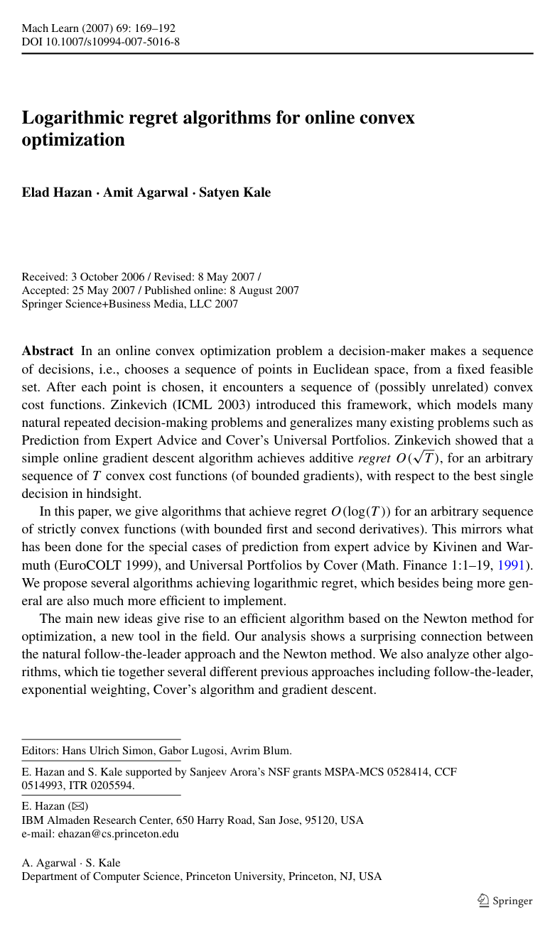
In an online convex optimization problem a decision-maker makes a sequence of decisions, i.e., chooses a sequence of points in Euclidean space, from a fixed feasible set. After each point is chosen, it encounters a sequence of (possibly unrelated) convex cost functions. Zinkevich (ICML 2003) introduced this framework, which models many natural repeated decision-making problems and generalizes many existing problems such as Prediction from Expert Advice and Cover's Universal Portfolios. Zinkevich showed that a simple online gradient descent algorithm achieves additive regret O(√T), for an arbitrary sequence of T convex cost functions (of bounded gradients), with respect to the best single decision in hindsight.

In this paper, we give algorithms that achieve regret O(log(T)) for an arbitrary sequence of strictly convex functions (with bounded first and second derivatives). This mirrors what has been done for the special cases of prediction from expert advice by Kivinen and Warmuth (EuroCOLT 1999), and Universal Portfolios by Cover (Math. Finance 1:1–19, 1991). We propose several algorithms achieving logarithmic regret, which besides being more general are also much more efficient to implement.

The main new ideas give rise to an efficient algorithm based on the Newton method for optimization, a new tool in the field. Our analysis shows a surprising connection between the natural follow-the-leader approach and the Newton method. We also analyze other algorithms, which tie together several different previous approaches including follow-the-leader, exponential weighting, Cover's algorithm and gradient descent.

Table of Contents

  • 1 Introduction
  • 1.1 Follow the leader
  • 2 Preliminaries
  • 2.1 Online convex optimization
  • 2.2 Notation and definitions
  • 2.3 Summary of our results
  • 3 The algorithms
  • 3.1 Online Gradient Descent
  • 3.2 Online Newton Step
  • 3.2.1 Implementation and running time
  • 3.3 Follow the Approximate Leader
  • 3.3.1 Analysis of Follow the Approximate Leader
  • 3.3.2 Implementation and running time
  • 3.4 Exponentially Weighted Online Optimization
  • 3.4.1 Implementation and running time
  • 4 Computing projections
  • 5 Conclusions
  • Appendix 1 Reductions for Follow the Leader
  • Appendix 2 Bounds on the potential function
  • References

Knowls

  1. Knowl 1 — Online Newton Step Algorithm

    algorithm

    The Online Newton Step (ONS) algorithm is an online convex optimization procedure designed for α\alpha-exp-concave cost functions over a convex feasible set P⊂Rn\mathcal{P} \subset \mathbb{R}^n with Euclidean diameter D=max⁡x,y∈P∥x−y∥2D = \max_{x,y \in \mathcal{P}} \|x - y\|_2 and gradient bound G=sup⁡x∈P,t∥∇ft(x)_2G = \sup_{x \in \mathcal{P}, t} \|\nabla f_t(x)\_2.

    ONS maintains a running sum of rank-one gradient outer products regularized by εIn\varepsilon I_n: At=∑τ=1t∇τ∇τ⊤+εInA_t = \sum_{\tau=1}^t \nabla_\tau \nabla_\tau^\top + \varepsilon I_n, where ε=1β2D2\varepsilon = \frac{1}{\beta^2 D^2} and β=12min⁡{14GD,α}\beta = \frac{1}{2} \min\left\{\frac{1}{4GD}, \alpha\right\}. The inverse At−1A_t^{-1} is updated in O(n2)O(n^2) time using the Sherman-Morrison formula. The unconstrained step moves in the Newton-like direction −1βAt−1∇t- \frac{1}{\beta} A_t^{-1} \nabla_t, followed by a generalized projection ΠPAt(y)=arg⁡min⁡x∈P(y−x)⊤At(y−x)\Pi_{\mathcal{P}}^{A_t}(y) = \arg\min_{x \in \mathcal{P}} (y - x)^\top A_t (y - x). The overall per-iteration running time is O~(n2)+Tprojg\tilde{O}(n^2) + T_{\text{proj}}^g, where TprojgT_{\text{proj}}^g is the time required to compute the generalized projection.

    Input: Convex set P⊂Rn\mathcal{P} \subset \mathbb{R}^n, diameter DD, gradient bound GG, exp-concavity parameter α\alpha, initial point x1∈Px_1 \in \mathcal{P}
    Set β=12min⁡{14GD,α}\beta = \frac{1}{2} \min\left\{\frac{1}{4GD}, \alpha\right\}
    Set ε=1β2D2\varepsilon = \frac{1}{\beta^2 D^2}
    Set A0=εInA_0 = \varepsilon I_n and A0−1=1εInA_0^{-1} = \frac{1}{\varepsilon} I_n
    for t=1,2,…,Tt = 1, 2, \dots, T do
        Play point xt∈Px_t \in \mathcal{P}
        Receive cost function ftf_t and compute gradient ∇t=∇ft(xt)\nabla_t = \nabla f_t(x_t)
        Update At=At−1+∇t∇t⊤A_t = A_{t-1} + \nabla_t \nabla_t^\top
        Compute At−1=At−1−1−At−1−1∇t∇t⊤At−1−11+∇t⊤At−1−1∇tA_t^{-1} = A_{t-1}^{-1} - \frac{A_{t-1}^{-1} \nabla_t \nabla_t^\top A_{t-1}^{-1}}{1 + \nabla_t^\top A_{t-1}^{-1} \nabla_t}
        Compute yt+1=xt−1βAt−1∇ty_{t+1} = x_t - \frac{1}{\beta} A_t^{-1} \nabla_t
        Compute xt+1=arg⁡min⁡x∈P(yt+1−x)⊤At(yt+1−x)x_{t+1} = \arg\min_{x \in \mathcal{P}} (y_{t+1} - x)^\top A_t (y_{t+1} - x)
    end for
  2. Knowl 2 — Regret Guarantee for the Online Newton Step Algorithm

    theoretical result

    Let P⊂Rn\mathcal{P} \subset \mathbb{R}^n be a closed, bounded, non-empty convex set with Euclidean diameter D=max⁡x,y∈P∥x−y∥2D = \max_{x,y \in \mathcal{P}} \|x - y\|_2. Suppose an online decision-maker encounters a sequence of twice differentiable cost functions ft:P→Rf_t : \mathcal{P} \to \mathbb{R} for t=1,…,Tt = 1, \dots, T that are α\alpha-exp-concave (i.e., exp⁡(−αft(x))\exp(-\alpha f_t(x)) is concave on P\mathcal{P} for some α>0\alpha > 0) with gradient norms bounded by sup⁡x∈P∥∇ft(x)_2≤G\sup_{x \in \mathcal{P}} \|\nabla f_t(x)\_2 \le G.

    When using the Online Newton Step algorithm with parameter β=12min⁡{14GD,α}\beta = \frac{1}{2}\min\left\{\frac{1}{4GD}, \alpha\right\} and regularization ε=1β2D2\varepsilon = \frac{1}{\beta^2 D^2}, the regret with respect to the best single fixed point in hindsight satisfies: RegretT(ONS)=∑t=1Tft(xt)−min⁡x∈P∑t=1Tft(x)≤5(1α+GD)nlog⁡T\text{Regret}_T(\text{ONS}) = \sum_{t=1}^T f_t(x_t) - \min_{x \in \mathcal{P}} \sum_{t=1}^T f_t(x) \le 5\left(\frac{1}{\alpha} + GD\right) n \log T

  3. Knowl 3 — Follow the Approximate Leader Algorithm

    algorithm

    Follow the Approximate Leader (FTAL) is an online convex optimization algorithm that operates on α\alpha-exp-concave cost functions by playing the minimizer of cumulative quadratic paraboloid lower bounds f~τ(x)\tilde{f}_\tau(x) constructed at each past step τ=1,…,t−1\tau = 1, \dots, t-1: f~τ(x)=fτ(xτ)+∇fτ(xτ)⊤(x−xτ)+β2(x−xτ)⊤∇fτ(xτ)∇fτ(xτ)⊤(x−xτ)\tilde{f}_\tau(x) = f_\tau(x_\tau) + \nabla f_\tau(x_\tau)^\top (x - x_\tau) + \frac{\beta}{2} (x - x_\tau)^\top \nabla f_\tau(x_\tau) \nabla f_\tau(x_\tau)^\top (x - x_\tau) where β=12min⁡{14GD,α}\beta = \frac{1}{2}\min\left\{\frac{1}{4GD}, \alpha\right\}.

    At round tt, the decision xt=arg⁡min⁡x∈P∑τ=1t−1f~τ(x)x_t = \arg\min_{x \in \mathcal{P}} \sum_{\tau=1}^{t-1} \tilde{f}_\tau(x) is algebraically equivalent to performing a generalized projection: xt=ΠPAt−1(At−1−1bt−1)=arg⁡min⁡x∈P(x−At−1−1bt−1)⊤At−1(x−At−1−1bt−1)x_t = \Pi_{\mathcal{P}}^{A_{t-1}}(A_{t-1}^{-1} b_{t-1}) = \arg\min_{x \in \mathcal{P}} (x - A_{t-1}^{-1} b_{t-1})^\top A_{t-1} (x - A_{t-1}^{-1} b_{t-1}) where At−1=∑τ=1t−1∇τ∇τ⊤A_{t-1} = \sum_{\tau=1}^{t-1} \nabla_\tau \nabla_\tau^\top, bt−1=∑τ=1t−1(∇τ∇τ⊤xτ−1β∇τ)b_{t-1} = \sum_{\tau=1}^{t-1} \left(\nabla_\tau \nabla_\tau^\top x_\tau - \frac{1}{\beta}\nabla_\tau\right), and At−1−1A_{t-1}^{-1} denotes the Moore-Penrose pseudoinverse of At−1A_{t-1}.

    Input: Convex set P⊂Rn\mathcal{P} \subset \mathbb{R}^n, parameter β>0\beta > 0, initial point x1∈Px_1 \in \mathcal{P}
    Set A0=0n×nA_0 = 0_{n \times n} and b0=0nb_0 = 0_n
    for t=1,2,…,Tt = 1, 2, \dots, T do
        Play point xt∈Px_t \in \mathcal{P}
        Observe cost function ftf_t and evaluate gradient ∇t=∇ft(xt)\nabla_t = \nabla f_t(x_t)
        Update At=At−1+∇t∇t⊤A_t = A_{t-1} + \nabla_t \nabla_t^\top
        Update bt=bt−1+∇t∇t⊤xt−1β∇tb_t = b_{t-1} + \nabla_t \nabla_t^\top x_t - \frac{1}{\beta}\nabla_t
        Compute xt+1=arg⁡min⁡x∈P(x−At−1bt)⊤At(x−At−1bt)x_{t+1} = \arg\min_{x \in \mathcal{P}} (x - A_t^{-1} b_t)^\top A_t (x - A_t^{-1} b_t)
    end for
  4. Knowl 4 — Regret Guarantee for Follow the Approximate Leader

    theoretical result

    Let P⊂Rn\mathcal{P} \subset \mathbb{R}^n be a closed, bounded, non-empty convex set with Euclidean diameter D=max⁡x,y∈P∥x−y∥2D = \max_{x,y \in \mathcal{P}} \|x - y\|_2. Suppose that for each t=1,…,Tt = 1, \dots, T, the cost function ft:P→Rf_t : \mathcal{P} \to \mathbb{R} is twice differentiable, α\alpha-exp-concave (meaning exp⁡(−αft(x))\exp(-\alpha f_t(x)) is concave on P\mathcal{P} for some α>0\alpha > 0), and satisfies sup⁡x∈P∥∇ft(x)_2≤G\sup_{x \in \mathcal{P}} \|\nabla f_t(x)\_2 \le G.

    When Follow the Approximate Leader is executed with parameter β=12min⁡{14GD,α}\beta = \frac{1}{2} \min\left\{\frac{1}{4GD}, \alpha\right\}, the regret with respect to the best single decision in hindsight satisfies: RegretT(FTAL)=∑t=1Tft(xt)−min⁡x∈P∑t=1Tft(x)≤64(1α+GD)n(log⁡T+1)\text{Regret}_T(\text{FTAL}) = \sum_{t=1}^T f_t(x_t) - \min_{x \in \mathcal{P}} \sum_{t=1}^T f_t(x) \le 64\left(\frac{1}{\alpha} + GD\right) n (\log T + 1)

  5. Knowl 5 — Second-Order Quadratic Lower Bound for Exp-Concave Functions

    theoretical result

    Let P⊂Rn\mathcal{P} \subset \mathbb{R}^n be a convex set of diameter D=max⁡x,y∈P∥x−y∥2D = \max_{x,y \in \mathcal{P}} \|x - y\|_2, and let f:P→Rf : \mathcal{P} \to \mathbb{R} be a differentiable function whose gradient is bounded by sup⁡x∈P∥∇f(x)_2≤G\sup_{x \in \mathcal{P}} \|\nabla f(x)\_2 \le G.

    If ff is α\alpha-exp-concave on P\mathcal{P} (i.e., exp⁡(−αf(x))\exp(-\alpha f(x)) is concave for α>0\alpha > 0), then for any parameter β\beta satisfying β≤12min⁡{14GD,α}\beta \le \frac{1}{2} \min\left\{\frac{1}{4GD}, \alpha\right\}, the function ff admits a quadratic lower bound around any point y∈Py \in \mathcal{P} relying only on its gradient: f(x)≥f(y)+∇f(y)⊤(x−y)+β2(x−y)⊤∇f(y)∇f(y)⊤(x−y),∀x,y∈Pf(x) \ge f(y) + \nabla f(y)^\top (x - y) + \frac{\beta}{2} (x - y)^\top \nabla f(y) \nabla f(y)^\top (x - y), \quad \forall x, y \in \mathcal{P} This inequality enables curvature-based online second-order optimization by replacing the full Hessian ∇2f(y)\nabla^2 f(y) with the outer product ∇f(y)∇f(y)⊤\nabla f(y) \nabla f(y)^\top.

  6. Knowl 6 — Comparison of Online Convex Optimization Algorithms with Logarithmic Regret

    data/table
    Algorithm Regret bound Running time
    OGD O(G2Hlog⁡T)O\left(\frac{G^2}{H} \log T\right) O~(n)+Tproj\tilde{O}(n) + T_{\text{proj}}
    ONS O((1α+GD)nlog⁡T)O\left(\left(\frac{1}{\alpha} + GD\right)n \log T\right) O~(n2)+Tprojg\tilde{O}(n^2) + T_{\text{proj}}^g
    FTAL O((1α+GD)nlog⁡T)O\left(\left(\frac{1}{\alpha} + GD\right)n \log T\right) O~(n2)+Tprojg\tilde{O}(n^2) + T_{\text{proj}}^g
    EWOO O(nαlog⁡T)O\left(\frac{n}{\alpha} \log T\right) poly(T,n)\text{poly}(T,n)

    This table compares four algorithms for online convex optimization over TT iterations in Rn\mathbb{R}^n in terms of their worst-case regret bounds and per-round computational complexities:

    • DD is the domain diameter max⁡x,y∈P∥x−y∥2\max_{x,y \in \mathcal{P}} \|x-y\|_2, GG is the gradient norm upper bound sup⁡x,t∥∇ft(x)_2\sup_{x, t} \|\nabla f_t(x)\_2, HH is the strong convexity parameter (where ∇2ft(x)⪰HIn\nabla^2 f_t(x) \succeq H I_n), and α\alpha is the exp-concavity parameter (where ∇2[exp⁡(−αft(x))]⪯0\nabla^2 [\exp(-\alpha f_t(x))] \preceq 0).
    • TprojT_{\text{proj}} is the time required for a standard Euclidean projection onto P\mathcal{P}; TprojgT_{\text{proj}}^g is the time required for a generalized projection under a matrix-induced norm. O~\tilde{O} hides constant and polylogarithmic factors in n,T,G,H,D,αn, T, G, H, D, \alpha.
    • Online Gradient Descent (OGD) achieves O(log⁡T)O(\log T) regret with fast O(n)O(n) updates but requires the strongest assumption (HH-strong convexity). Online Newton Step (ONS) and Follow the Approximate Leader (FTAL) relax this to α\alpha-exp-concavity with bounded gradients while maintaining polynomial O~(n2)\tilde{O}(n^2) efficiency. Exponentially Weighted Online Optimization (EWOO) requires only α\alpha-exp-concavity without requiring bounded gradients, but requires polynomial-time sampling poly(T,n)\text{poly}(T,n) per step.
  7. Knowl 7 — Exponentially Weighted Online Optimization Algorithm

    algorithm

    Exponentially Weighted Online Optimization (EWOO) is an online optimization algorithm for α\alpha-exp-concave cost functions over a convex domain P⊂Rn\mathcal{P} \subset \mathbb{R}^n. At round tt, it computes the continuous center of mass under weights defined exponentially on the cumulative past loss: wt(x)=exp⁡(−α∑τ=1t−1fτ(x))w_t(x) = \exp\left(-\alpha \sum_{\tau=1}^{t-1} f_\tau(x)\right) The decision played at round tt is: xt=∫Pxwt(x) dx∫Pwt(x) dxx_t = \frac{\int_{\mathcal{P}} x w_t(x) \, dx}{\int_{\mathcal{P}} w_t(x) \, dx} Selecting xtx_t randomly according to the probability density proportional to wt(x)w_t(x) yields the same regret bound in expectation. The point xtx_t can be sampled in polynomial time O~((n4+mn3)log⁡(R/r))\tilde{O}((n^4 + mn^3)\log(R/r)) using Markov chain random walks.

    Input: Convex set P⊂Rn\mathcal{P} \subset \mathbb{R}^n, exp-concavity parameter α>0\alpha > 0
    for t=1,2,…,Tt = 1, 2, \dots, T do
        Define weight function wt(x)=exp⁡(−α∑τ=1t−1fτ(x))w_t(x) = \exp\left(-\alpha \sum_{\tau=1}^{t-1} f_\tau(x)\right)
        Compute and play xt=∫Pxwt(x)dx∫Pwt(x)dxx_t = \frac{\int_{\mathcal{P}} x w_t(x) dx}{\int_{\mathcal{P}} w_t(x) dx}
        Observe convex cost function ft:P→Rf_t : \mathcal{P} \to \mathbb{R}
    end for
  8. Knowl 8 — Regret Bound for Exponentially Weighted Online Optimization

    theoretical result

    Let P⊂Rn\mathcal{P} \subset \mathbb{R}^n be a closed, bounded, non-empty convex set. Suppose that for all t=1,…,Tt = 1, \dots, T, each cost function ft:P→Rf_t : \mathcal{P} \to \mathbb{R} is α\alpha-exp-concave, meaning exp⁡(−αft(x))\exp(-\alpha f_t(x)) is concave over P\mathcal{P} for some constant α>0\alpha > 0. No bound on the gradient magnitude of ftf_t is required.

    The regret of the Exponentially Weighted Online Optimization (EWOO) algorithm with respect to the best single decision in hindsight satisfies: RegretT(EWOO)=∑t=1Tft(xt)−min⁡x∈P∑t=1Tft(x)≤nα(1+log⁡(T+1))\text{Regret}_T(\text{EWOO}) = \sum_{t=1}^T f_t(x_t) - \min_{x \in \mathcal{P}} \sum_{t=1}^T f_t(x) \le \frac{n}{\alpha}(1 + \log(T + 1)) The identical bound holds in expectation if xtx_t is chosen as a single random point sampled from the density proportional to exp⁡(−α∑τ=1t−1fτ(x))\exp\left(-\alpha \sum_{\tau=1}^{t-1} f_\tau(x)\right).

  9. Knowl 9 — Logarithmic Regret of Online Gradient Descent for Strongly Convex Functions

    theoretical result

    Let P⊂Rn\mathcal{P} \subset \mathbb{R}^n be a closed, bounded, non-empty convex set. Suppose that each cost function ft:P→Rf_t : \mathcal{P} \to \mathbb{R} is HH-strongly convex (i.e., ∇2ft(x)⪰HIn\nabla^2 f_t(x) \succeq H I_n for all x∈Px \in \mathcal{P} with H>0H > 0) and has bounded gradients sup⁡x∈P∥∇ft(x)_2≤G\sup_{x \in \mathcal{P}} \|\nabla f_t(x)\_2 \le G.

    When Online Gradient Descent is run with step sizes ηt=1Ht\eta_t = \frac{1}{Ht} and update rule: xt=ΠP(xt−1−ηt∇ft−1(xt−1))=arg⁡min⁡x∈P∥x−(xt−1−ηt∇ft−1(xt−1))∥2x_t = \Pi_{\mathcal{P}}\left(x_{t-1} - \eta_t \nabla f_{t-1}(x_{t-1})\right) = \arg\min_{x \in \mathcal{P}} \|x - (x_{t-1} - \eta_t \nabla f_{t-1}(x_{t-1}))\|_2 the worst-case regret over TT iterations satisfies: RegretT(OGD)=∑t=1Tft(xt)−min⁡x∈P∑t=1Tft(x)≤G22H(1+log⁡T)\text{Regret}_T(\text{OGD}) = \sum_{t=1}^T f_t(x_t) - \min_{x \in \mathcal{P}} \sum_{t=1}^T f_t(x) \le \frac{G^2}{2H}(1 + \log T)

  10. Knowl 10 — Regret Bound for Follow the Leader on Functions with Univariate Curvature

    theoretical result

    Let P⊂Rn\mathcal{P} \subset \mathbb{R}^n be a closed, bounded convex set with diameter D=max⁡x,y∈P∥x−y∥2D = \max_{x,y \in \mathcal{P}} \|x - y\|_2. Suppose that each cost function ft:P→Rf_t : \mathcal{P} \to \mathbb{R} has the form ft(x)=gt(vt⊤x)f_t(x) = g_t(v_t^\top x) for a univariate convex function gt:R→Rg_t : \mathbb{R} \to \mathbb{R} and vector vt∈Rnv_t \in \mathbb{R}^n satisfying ∥vt∥2≤R\|v_t\|_2 \le R.

    If for all x∈Px \in \mathcal{P} and t∈[T]t \in [T], the derivatives satisfy ∣gt′(vt⊤x)∣≤b|g_t'(v_t^\top x)| \le b and gt′′(vt⊤x)≥a>0g_t''(v_t^\top x) \ge a > 0, then the standard Follow the Leader (FTL) algorithm, which plays xt=arg⁡min⁡x∈P∑τ=1t−1fτ(x)x_t = \arg\min_{x \in \mathcal{P}} \sum_{\tau=1}^{t-1} f_\tau(x), achieves the regret guarantee: RegretT(FTL)=∑t=1Tft(xt)−min⁡x∈P∑t=1Tft(x)≤2nb2a(log⁡(DRaTb)+1)\text{Regret}_T(\text{FTL}) = \sum_{t=1}^T f_t(x_t) - \min_{x \in \mathcal{P}} \sum_{t=1}^T f_t(x) \le \frac{2n b^2}{a}\left(\log\left(\frac{D R a T}{b}\right) + 1\right)

  11. Knowl 11 — Contraction of Generalized Projections under Positive Semidefinite Metrics

    theoretical result

    Let P⊆Rn\mathcal{P} \subseteq \mathbb{R}^n be a non-empty convex set and let A∈Rn×nA \in \mathbb{R}^{n \times n} be a positive semidefinite matrix (A⪰0A \succeq 0). For any point y∈Rny \in \mathbb{R}^n, the generalized projection of yy onto P\mathcal{P} in the norm induced by AA is defined by: ΠPA[y]=arg⁡min⁡x∈P(x−y)⊤A(x−y)\Pi_{\mathcal{P}}^A[y] = \arg\min_{x \in \mathcal{P}} (x - y)^\top A (x - y) For any reference point a∈Pa \in \mathcal{P} and projected point z=ΠPA[y]z = \Pi_{\mathcal{P}}^A[y], the generalized projection satisfies the non-expansion contraction property: (y−a)⊤A(y−a)≥(z−a)⊤A(z−a)(y - a)^\top A (y - a) \ge (z - a)^\top A (z - a)

  12. Knowl 12 — Logarithmic Potential Sum for Rank-One Matrix Updates

    theoretical result

    Let u1,u2,…,uT∈Rnu_1, u_2, \dots, u_T \in \mathbb{R}^n be an arbitrary sequence of vectors satisfying ∥ut∥2≤r\|u_t\|_2 \le r for all t∈[T]t \in [T] with r>0r > 0. For any regularization parameter ε>0\varepsilon > 0, let Vt=∑τ=1tuτuτ⊤+εInV_t = \sum_{\tau=1}^t u_\tau u_\tau^\top + \varepsilon I_n.

    Then the cumulative sum of quadratic forms evaluated on the inverse sequence Vt−1V_t^{-1} is bounded logarithmically in TT: ∑t=1Tut⊤Vt−1ut≤nlog⁡(r2Tε+1)\sum_{t=1}^T u_t^\top V_t^{-1} u_t \le n \log\left(\frac{r^2 T}{\varepsilon} + 1\right) This bound is derived using the matrix determinant inequality A−1∙(A−B)≤log⁡∣A∣∣B∣A^{-1} \bullet (A - B) \le \log\frac{|A|}{|B|} which holds for any pair of positive definite matrices A⪰B≻0A \succeq B \succ 0, where A∙B=Tr(AB)=∑i,j=1nAijBijA \bullet B = \text{Tr}(A B) = \sum_{i,j=1}^n A_{ij} B_{ij} and ∣A∣|A| denotes the determinant of AA.

Coverage note — None was omitted; all main contributed algorithms, regret theorems, structural characterizations of exp-concavity, and potential lemmas have been captured.

References

  1. 1.Blum, A., & Kalai, A. (1997). Universal portfolios with and without transaction costs. In COLT ’97: proceedings of the tenth annual conference on computational learning theory (pp. 309–313). New York: ACM.
  2. 2.Brookes, M. (2005). The matrix reference manual. http://www.ee.ic.ac.uk/hp/staff/dmb/matrix/intro.html.
  3. 3.Boyd, S., & Vandenberghe, L. (2004). Convex optimization. New York: Cambridge University Press.
  4. 4.Cesa-Bianchi, N., & Lugosi, G. (2006). Prediction, learning, and games. Cambridge: Cambridge University Press.
  5. 5.Cover, T. (1991). Universal portfolios. Mathematical Finance, 1, 1–19.
  6. 6.Gaivoronski, A. A., & Stella, F. (2000). Stochastic nonstationary optimization for finding universal portfolios. Annals of Operations Research, 100, 165–188.
  7. 7.Hannan, J. (1957). Approximation to bayes risk in repeated play. In M. Dresher, A.W. Tucker, & P. Wolfe (Eds.), Contributions to the theory of games (Vol. III, pp. 97–139).
  8. 8.Hazan, E. (2006). Efficient algorithms for online convex optimization and their applications. PhD thesis, Princeton University.
  9. 9.Kakade, S. (2005). Personal communication.
  10. 10.Kalai, A., & Vempala, S. (2003). Efficient algorithms for universal portfolios. Journal of Machine Learning Research, 3, 423–440.
  11. 11.Kalai, A., & Vempala, S. (2005). Efficient algorithms for on-line optimization. Journal of Computer and System Sciences, 71(3), 291–307.
  12. 12.Kivinen, J., & Warmuth, M. K. (1998). Relative loss bounds for multidimensional regression problems. In M. I. Jordan, M. J. Kearns, & S.A. Solla (Eds.), Advances in neural information processing systems (Vol. 10). Cambridge: MIT.
  13. 13.Kivinen, J., & Warmuth, M. K. (1999). Averaging expert predictions. In Computational learning theory: 4th European conference (EuroCOLT ’99) (pp. 153–167). Berlin: Springer.
  14. 14.Lovász, L., & Vempala, S. (2003a). The geometry of logconcave functions and an o∗(n3) sampling algorithm. Technical Report MSR-TR-2003-04, Microsoft Research.
  15. 15.Lovász, L., & Vempala, S. (2003b). Simulated annealing in convex bodies and an 0∗(n4) volume algorithm. In Proceedings of the 44th symposium on foundations of computer science (FOCS) (pp. 650–659).
  16. 16.Lobo, M. S., Vandenberghe, L., Boyd, S., & Lebret, H. (1998). Applications of second-order cone programming.
  17. 17.Merhav, N., & Feder, M. (1992). Universal sequential learning and decision from individual data sequences. In COLT ’92: Proceedings of the fifth annual workshop on computational learning theory (pp. 413–427). New York: ACM.
  18. 18.Riedel, K. (1991). A Sherman–Morrison–Woodbury identity for rank augmenting matrices with application to centering. SIAM Journal on Mathematical Analysis, 12(1), 80–95.
  19. 19.Vaidya, P. M. (1996). A new algorithm for minimizing convex functions over convex sets. Mathematical Programming, 73(3), 291–341.
  20. 20.Zinkevich, M. (2003). Online convex programming and generalized infinitesimal gradient ascent. In Proceedings of the twentieth international conference on machine learning (ICML) (pp. 928–936).

Citation

MLA
Hazan, E., et al. “Logarithmic Regret Algorithms for Online Convex Optimization”. Machine Learning, vol. 69, nos. 2-3, 2007, pp. 169–92, https://doi.org/10.1007/s10994-007-5016-8.
APA
Hazan, E., Agarwal, A., & Kale, S. (2007). Logarithmic regret algorithms for online convex optimization. Machine Learning, 69(2-3), 169–192. https://doi.org/10.1007/s10994-007-5016-8
Chicago
Hazan, E., A. Agarwal, and S. Kale. 2007. “Logarithmic Regret Algorithms for Online Convex Optimization”. Machine Learning 69 (2-3): 169–92. https://doi.org/10.1007/s10994-007-5016-8.
Harvard
Hazan, E., Agarwal, A. and Kale, S. (2007) “Logarithmic regret algorithms for online convex optimization”, Machine Learning, 69(2-3), pp. 169–192. Available at: https://doi.org/10.1007/s10994-007-5016-8.
Vancouver
1. Hazan E, Agarwal A, Kale S (2007) Logarithmic regret algorithms for online convex optimization. Machine Learning 69:169–192

BibTeX

@article{Hazan_2007, title={Logarithmic regret algorithms for online convex optimization}, volume={69}, ISSN={1573-0565}, url={http://dx.doi.org/10.1007/s10994-007-5016-8}, DOI={10.1007/s10994-007-5016-8}, number={2-3}, journal={Machine Learning}, publisher={Springer Science and Business Media LLC}, author={Hazan, Elad and Agarwal, Amit and Kale, Satyen}, year={2007}, month=Aug, pages={169–192} }
Metadata:Crossref

Access the Paper

This paper is available from its original source. Click below to access the PDF.

Open PDF