Inductive Moment Matching

article2025ICML116 citations

Introduces Inductive Moment Matching, a single-stage framework that trains few-step generative models from scratch without pre-training or distillation, achieving state-of-the-art fast sampling performance on ImageNet and CIFAR-10 with guaranteed distribution-level convergence.

Listen

Modern generative artificial intelligence models for images, video, and audio typically face a fundamental trade-off among output quality, generation speed, and training stability. Standard diffusion models produce high-quality samples but require dozens or hundreds of computational steps during generation, making deployment slow and expensive. Existing solutions attempt to compress these models through distillation or alternative training techniques, but they frequently suffer from training instability, mode collapse, and complex multi-stage pipelines requiring extensive tuning.

The article introduces and evaluates Inductive Moment Matching, a framework designed to train fast, high-fidelity generative models from scratch in a single stage. The main objective is to establish a mathematically principled method that enables direct sample generation in one or very few computational steps while ensuring stable optimization without specialized regularization tricks.

To achieve this, the approach relies on mathematical induction over time-dependent probability distributions using stochastic paths. Instead of matching individual data points, the method applies Maximum Mean Discrepancy, an integral probability metric, to align all statistical moments between intermediate noisy distributions and cleaner targets across small time intervals. Credibility was established through extensive experiments across standard image benchmarks, specifically CIFAR-10 and ImageNet at 256×256 resolution, utilizing standard Transformer architectures such as Diffusion Transformers without modifying core network designs.

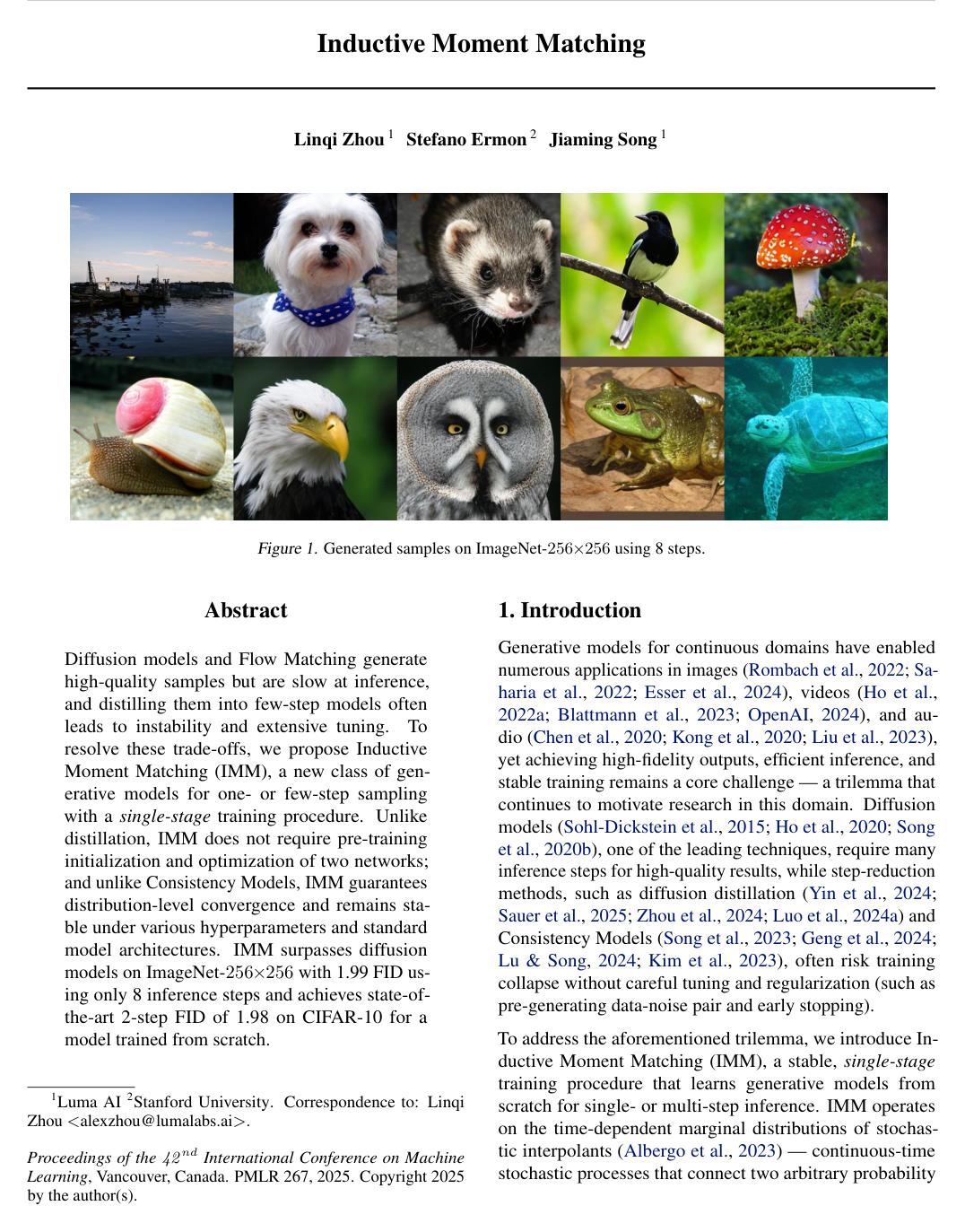
The key findings demonstrate major gains in speed, quality, and stability. On ImageNet-256×256, the method achieved a state-of-the-art Fréchet Inception Distance score of 1.99 using only 8 sampling steps, outperforming baseline diffusion models that require 250 steps as well as competing visual autoregressive models. On CIFAR-10, it attained a record 1.98 score with only 2 generation steps when trained from scratch. The analysis also revealed that training remained highly stable across various architectural embeddings and particle batch sizes, whereas existing consistency models collapsed under identical conditions because they effectively match only first moments rather than the full distribution.

These results have substantial implications for artificial intelligence infrastructure costs and real-time product feasibility. By cutting inference steps from hundreds down to 2 to 8 steps, computing costs and latency drop significantly without sacrificing visual fidelity. Furthermore, training from scratch in a single stage removes the operational friction, failure risk, and resource overhead of maintaining complex two-stage distillation pipelines.

For practical implementation, organizations looking to reduce generative model latency should adopt the Inductive Moment Matching training recipe and prioritize optimal particle batch sizes (such as four particles per group) and Laplace kernel formulations. When adopting lower-precision hardware training (such as FP16), practitioners must maintain a small minimum time gap to preserve numerical distinguishability between nearby time steps. Further exploration should pilot this methodology on large-scale text-to-image and video domains, alongside investigating combinations of restart samplers with pushforward sampling.

Luma AI Stanford University diffusion probabilistic models generative model inference inductive moment matching Generative Moment Matching Network flow matching

arXiv: 2503.07565

Paper: Consistency Models, Yang Song et al. (2023). Introduces consistency models for fast, few-step generation that match trajectory endpoints, establishing the core paradigm and failure modes that Inductive Moment Matching directly aims to resolve via full distribution alignment.
Paper: Flow Matching for Generative Modeling, Yaron Lipman et al. (2023). Presents the foundational continuous-time flow matching framework along probability paths that provides the continuous trajectory background for inductive moment matching.
Paper: Progressive Distillation for Fast Sampling of Diffusion Models, Tim Salimans et al. (2022). Establishes progressive distillation to compress diffusion sampling steps, representing the multi-stage acceleration baseline that Inductive Moment Matching seeks to replace with single-stage training from scratch.
Paper: Elucidating the Design Space of Diffusion-Based Generative Models, Tero Karras et al. (2022). Provides the modern standardized formulations, noise schedules, and numerical integration principles essential for understanding continuous-time diffusion dynamics.
Paper: Score-Based Generative Modeling through Stochastic Differential Equations, Yang Song et al. (2021). Formulates continuous-time diffusion via stochastic and ordinary differential equations, providing the theoretical bedrock for stochastic paths between intermediate noise distributions.
Paper: Flow Straight and Fast: Learning to Generate and Transfer Data with Rectified Flow, Xingchao Liu et al. (2023). Introduces rectified flow and straight-line trajectory learning, serving as an important conceptual precursor to fast, few-step path-based generative modeling.
Paper: Denoising Diffusion Implicit Models, Jiaming Song et al. (2021). Pioneers accelerated non-Markovian deterministic sampling for diffusion models, establishing the foundation for few-step generative trajectories.
Paper: Denoising Diffusion Probabilistic Models, Jonathan Ho et al. (2020). Introduces the foundational denoising diffusion probabilistic model formulation upon which subsequent fast-sampling and path-matching techniques are built.

Paper: Mean Flows for One-step Generative Modeling, Zhengyang Geng et al. (2025). Introduces MeanFlow for one-step generative modeling by learning average velocities over time intervals, directly comparing against and advancing beyond Inductive Moment Matching.
Paper: Generative Modeling via Drifting, Mingyang Deng et al. (2026). Extends the pursuit of single-stage, one-step generation by formulating a drifting field mechanism that aligns generated and real distributions during training.
Paper: Adjoint Matching: Fine-tuning Flow and Diffusion Generative Models with Memoryless Stochastic Optimal Control, Carles Domingo-Enrich et al. (2025). Applies memoryless stochastic optimal control to fine-tune continuous flow and dynamical generative models like those trained by Inductive Moment Matching to human preference distributions.
Paper: Variational Flow Maps: Make Some Noise for One-Step Conditional Generation, Abbas Mammadov et al. (2026). Extends fast one-step flow-based mapping architectures to solve challenging conditional generation and noisy inverse problems via learned noise adapters.

Abstract

Diffusion models and Flow Matching generate high-quality samples but are slow at inference, and distilling them into few-step models often leads to instability and extensive tuning. To resolve these trade-offs, we propose Inductive Moment Matching (IMM), a new class of generative models for one- or few-step sampling with a single-stage training procedure. Unlike distillation, IMM does not require pre-training initialization and optimization of two networks; and unlike Consistency Models, IMM guarantees distribution-level convergence and remains stable under various hyperparameters and standard model architectures. IMM surpasses diffusion models on ImageNet-256×256 with 1.99 FID using only 8 inference steps and achieves state-of-the-art 2-step FID of 1.98 on CIFAR-10 for a model trained from scratch.

1. Introduction
2. Preliminaries
2.1. Diffusion, Flow Matching, and Interpolants
2.2. Maximum Mean Discrepancy
3. Inductive Moment Matching
3.1. Model Construction via Interpolants
3.2. Learning via Inductive Bootstrapping
4. Simplified Formulation and Practice
4.1. Algorithmic Considerations
4.2. Other Implementation Choices
4.3. Sampling
5. Connection with Prior Works
6. Related Works
7. Experiments
7.1. Image Generation
7.2. IMM Training is Stable
7.3. Sampling
7.4. Scaling Behavior
7.5. Ablation Studies
8. Conclusion
Impact Statement
Acknowledgement
References
A. Background: Properties of Stochastic Interpolants
B. Theorems and Derivations
B.1. Divergence Minimizer
B.2. Boundary Satisfaction of Model Distribution
B.3. Definition of Well-Conditioned r ( s, t )
B.4. Main Theorem
B.5. Self-Consistency Implies Marginal Preservation
B.6. Existence of Deterministic Minimizer
C. Analysis of Simplified Parameterization
C.1. DDIM Interpolant
C.2. Reusing x t for x r
C.3. Simplified Objective
C.4. Empirical Estimation
C.5. Simplified Parameterization
C.6. Mapping Function r ( s, t )
C.7. Time Distribution p ( s, t )
C.8. Kernel Function
C.9. Weighting Function w ( s, t )
D. Training Algorithm
E. Classifier-Free Guidance
F. Sampling Algorithms
G. Connection with Prior Works
G.1. Consistency Models
G.2. Diffusion GAN and Adversarial Consistency Distillation
G.3. Generative Moment Matching Network
H. Differential Inductive Moment Matching
H.1. Pseudo-Objective
H.2. Connection with Continuous-Time CMs
I. Experiment Settings
I.1. Training & Parameterization Settings
I.2. Inference Settings
I.3. Scaling Settings
I.4. Scaling Beyond 8 Steps
I.5. Ablation on exponent a
I.6. Caveats for Lower-Precision Training
J. Additional Visualization

Knowls

Knowl 1 — Inductive Moment Matching Objective
model/method
Inductive Moment Matching (IMM) is a single-stage framework for training one-step and few-step generative models from scratch. Let $q(x)$ be the data distribution on $\mathbb{R}^D$ , $p(\epsilon) = \mathcal{N}(0, \sigma_d^2 I)$ be a prior distribution with data standard deviation $\sigma_d$ , and $x_t = \alpha_t x + \sigma_t \epsilon$ be the time-interpolated variable at $t \in [0, 1]$ with marginal distribution $q_t(x_t)$ . IMM parameterizes a deterministic one-step sampler $f_{s,t}^\theta(x_t)$ that maps samples from $q_t(x_t)$ directly to intermediate or clean marginals $q_s(x_s)$ for any $s < t$ .

For timesteps $s \le r < t$ , the model matches the distribution produced by running the model from $t$ to $s$ with the bootstrapped distribution produced from $r$ to $s$ . Using Maximum Mean Discrepancy (MMD) with a positive definite kernel $k(\cdot, \cdot)$ and stop-gradient parameters $\theta^-$ , the training objective is:
$\mathcal{L}_{\text{IMM}}(\theta) = \mathbb{E}_{x_t, x'_t, x_r, x'_r, s, t}\left[ w(s, t) \left( k(y_{s,t}, y'_{s,t}) + k(y_{s,r}, y'_{s,r}) - k(y_{s,t}, y'_{s,r}) - k(y'_{s,t}, y_{s,r}) \right) \right]$
where $x_t, x'_t \sim q_t(x_t)$ are independent samples, $x_r = \text{DDIM}(x_t, x, r, t)$ and $x'_r = \text{DDIM}(x'_t, x', r, t)$ are intermediate states obtained by reusing $(x_t, x)$ and $(x'_t, x')$ , $y_{s,t} = f_{s,t}^\theta(x_t)$ , $y'_{s,t} = f_{s,t}^\theta(x'_t)$ , $y_{s,r} = f_{s,r}^{\theta^-}(x_r)$ , $y'_{s,r} = f_{s,r}^{\theta^-}(x'_r)$ , and $w(s, t)$ is a positive weighting function.
Knowl 2 — Marginal-Preserving and Self-Consistent Stochastic Interpolants
theoretical result
Let $x \sim q(x)$ and $\epsilon \sim p(\epsilon)$ define the endpoint marginals, and let $x_t \sim q_t(x_t|x, \epsilon) = \mathcal{N}(I_t(x, \epsilon), \gamma_t^2 I)$ be a stochastic interpolant with marginal $q_t(x_t)$ . A generalized interpolant $x_s \sim q_{s|t}(x_s|x, x_t) = \mathcal{N}(I_{s|t}(x, x_t), \gamma_{s|t}^2 I)$ for $s \in [0, t]$ is defined to satisfy $I_{t|t}(x, x_t) = x_t$ , $I_{0|t}(x, x_t) = x$ , and $\gamma_{t|t} = \gamma_{0|t} = 0$ .
1. Marginal Preservation: An interpolant is marginal-preserving if for all $t \in [0, 1]$ and all $s \in [0, t]$ :
$q_s(x_s) = \iint q_{s|t}(x_s|x, x_t) q_t(x|x_t) q_t(x_t) \,\mathrm{d}x_t \,\mathrm{d}x$
where $q_t(x|x_t) = \int q_t(x_t|x, \epsilon) q(x) p(\epsilon) / q_t(x_t) \,\mathrm{d}\epsilon$ .
1. Self-Consistency Condition: An interpolant is self-consistent if for all $0 \le s \le r \le t \le 1$ :
$q_{s|t}(x_s|x, x_t) = \int q_{s|r}(x_s|x, x_r) q_{r|t}(x_r|x, x_t) \,\mathrm{d}x_r$
Any self-consistent interpolant is necessarily marginal-preserving.
1. DDIM Interpolant: The deterministic Denoising Diffusion Implicit Model (DDIM) interpolator, defined with $\gamma_{s|t} \equiv 0$ and
$\text{DDIM}(x_t, x, s, t) = \left(\alpha_s - \frac{\sigma_s}{\sigma_t}\alpha_t\right)x + \frac{\sigma_s}{\sigma_t}x_t$
satisfies the self-consistency condition and guarantees the existence of a deterministic minimizer for the one-step sampling distribution $p_{s|t}^\theta(x|x_t) = \delta(x - g_\theta(x_t, s, t))$ .
Knowl 3 — Distribution-Level Convergence of Inductive Moment Matching
theoretical result
Let $r(s, t) = \max(s, t - \Delta(t))$ be a well-conditioned decrement function where $\Delta(t) \ge \epsilon > 0$ and $r(s, t)$ is strictly increasing for $t \ge \sup\{u : r(s, u) = s\}$ . Let the interpolant $q_{s|t}(x_s|x, x_t)$ be marginal-preserving, and let $\theta_n^*$ be the global minimizer at induction step $n$ of the loss:
$\mathcal{L}(\theta_n) = \mathbb{E}_{s, t}\left[ w(s, t) \text{MMD}^2(p_{s|r(s,t)}^{\theta_{n-1}^*}(x_s), p_{s|t}^{\theta_n}(x_s)) \right]$
Under infinite training data and infinite neural network capacity, for all $t \in [0, 1]$ and all $s \in [0, t]$ :
$\lim_{n \to \infty} \text{MMD}^2(q_s(x_s), p_{s|t}^{\theta_n^*}(x_s)) = 0$
Consequently, the learned implicit one-step sampler $p_{s|t}^{\theta_n}(x|x_t)$ guarantees convergence to the true target data distribution $q_s(x_s)$ across all intermediate and endpoint timesteps.
Knowl 4 — Consistency Models as a Single-Particle Special Case of IMM
theoretical result
Consistency Models (CMs) trained with discrete $L_2$ regression loss are a single-particle, first-moment matching reduction of the Inductive Moment Matching (IMM) framework:
1. $L_2$ Loss Reduction: When setting $x_t = x'_t$ , $x_r = x'_r$ (a single-particle batch size $M = 1$ ), fixing target time $s \to 0$ , and adopting the negative energy kernel $k(x, y) = -\|x - y\|^2$ , the IMM objective reduces to the standard Consistency Model training loss:
$\mathcal{L}_{\text{CM}}(\theta) = \mathbb{E}_{x_t, x, t}\left[ w(t) \|g_\theta(x_t, t) - g_{\theta^-}(x_r, r)\|^2 \right]$
This formulation drops the cross-particle repulsion term present in MMD and only matches the first moment of the distribution, explaining the empirical training instability and mode collapse observed in CMs.
1. Pseudo-Huber Loss as a Characteristic Kernel: The negative pseudo-Huber loss $k_c(x, y) = c - \sqrt{\|x - y\|^2 + c^2}$ ( $c > 0$ ) is a conditionally positive definite kernel. Its Taylor series expansion contains all even powers $\|x - y\|^{2j}$ ( $j \ge 1$ ), which implies that matching pseudo-Huber loss corresponds to matching all moments of the target and predicted distributions rather than the first moment alone.
Knowl 5 — IMM Training Algorithm
algorithm
The Inductive Moment Matching training algorithm samples mini-batches, splits them into particle groups that share sampled time tuples, computes intermediate states via self-consistent DDIM interpolation, and optimizes network parameters via the empirical MMD kernel loss.
Input: Model parameter $\theta$ , dataset $q(x)$ , prior $p(\epsilon) = \mathcal{N}(0, \sigma_d^2 I)$ , batch size $B$ , particle group size $M$ , mapping function $r(s, t)$ , flow schedule $\alpha_t, \sigma_t$ , kernel $k(\cdot, \cdot)$ , weighting function $w(s, t)$ , label dropout probability $p_\text{drop}$
Output: Optimized model parameters $\theta$
Initialize $\theta_0 \leftarrow \theta, n \leftarrow 0$
while model has not converged do
  Sample batch of $B$ instances: data $x$ , conditioning labels $c$ , and noise $\epsilon \sim \mathcal{N}(0, \sigma_d^2 I)$
  Partition the $B$ instances into $B/M$ independent groups of $M$ particles each
  for each group $i = 1, \dots, B/M$ do
    Sample $t_i \sim \mathcal{U}(\epsilon_t, T)$ and $s_i \sim \mathcal{U}(\epsilon_t, t_i)$
    Compute intermediate target time $r_i = r(s_i, t_i)$
    for each particle $j = 1, \dots, M$ in group $i$ do
       $x_{t_i}^{(i,j)} \leftarrow \alpha_{t_i} x^{(i,j)} + \sigma_{t_i} \epsilon^{(i,j)}$
       $x_{r_i}^{(i,j)} \leftarrow \text{DDIM}(x_{t_i}^{(i,j)}, x^{(i,j)}, r_i, t_i)$
      With probability $p_\text{drop}$ , set label $c^{(i,j)} \leftarrow \emptyset$
    end for
  end for
  Compute the empirical loss $\hat{\mathcal{L}}_{\text{IMM}}(\theta_n)$ over all $B/M$ groups:
   $\hat{\mathcal{L}}_{\text{IMM}}(\theta_n) = \frac{1}{B/M} \sum_{i=1}^{B/M} \frac{w(s_i, t_i)}{M^2} \sum_{j=1}^M \sum_{k=1}^M [ k(f_{s_i,t_i}^{\theta_n}(x_{t_i}^{(i,j)}), f_{s_i,t_i}^{\theta_n}(x_{t_i}^{(i,k)})) + k(f_{s_i,r_i}^{\theta_n^-}(x_{r_i}^{(i,j)}), f_{s_i,r_i}^{\theta_n^-}(x_{r_i}^{(i,k)})) - 2 k(f_{s_i,t_i}^{\theta_n}(x_{t_i}^{(i,j)}), f_{s_i,r_i}^{\theta_n^-}(x_{r_i}^{(i,k)})) ]$
  Update $\theta_{n+1}$ by taking an optimizer step on $\nabla_{\theta_n} \hat{\mathcal{L}}_{\text{IMM}}(\theta_n)$
   $n \leftarrow n + 1$
end while
Knowl 6 — Pushforward and Restart Sampling Algorithms for IMM
algorithm
IMM supports both deterministic pushforward sampling and stochastic restart sampling across arbitrary discrete time trajectories $\{t_i\}_{i=0}^N$ where $T = t_N > t_{N-1} > \dots > t_0 = \epsilon_t$ .
Input: Trained model $f_\theta$ , step sequence $\{t_i\}_{i=0}^N$ , prior variance $\sigma_d^2$ , guidance weight $w$
Output: Clean sample $x_0$
Procedure PushforwardSampling:
  Sample $x_{t_N} \sim \mathcal{N}(0, \sigma_d^2 I)$
  for $i = N, N-1, \dots, 1$ do
    if guidance enabled then
       $x_{t_{i-1}} \leftarrow f_{t_{i-1}, t_i, w}^\theta(x_{t_i})$
    else
       $x_{t_{i-1}} \leftarrow f_{t_{i-1}, t_i}^\theta(x_{t_i})$
    end if
  end for
  return $x_{t_0}$
Procedure RestartSampling:
  Sample $x_{t_N} \sim \mathcal{N}(0, \sigma_d^2 I)$
  for $i = N, N-1, \dots, 1$ do
    if guidance enabled then
       $\tilde{x} \leftarrow f_{t_0, t_i, w}^\theta(x_{t_i})$
    else
       $\tilde{x} \leftarrow f_{t_0, t_i}^\theta(x_{t_i})$
    end if
    if $i \neq 1$ then
      Sample $\tilde{\epsilon} \sim \mathcal{N}(0, \sigma_d^2 I)$
       $x_{t_{i-1}} \leftarrow \alpha_{t_{i-1}} \tilde{x} + \sigma_{t_{i-1}} \tilde{\epsilon}$
    else
       $x_{t_0} \leftarrow \tilde{x}$
    end if
  end for
  return $x_{t_0}$
Knowl 7 — Laplace Kernel, Loss Weighting, and Network Parameterizations in IMM
model/method
Practical implementation of Inductive Moment Matching incorporates specific kernel, weighting, and network formulations:
1. Laplace Kernel: Rather than RBF kernels, IMM adopts a time-dependent Laplace kernel with dimension $D$ :
$k_{s,t}(x, y) = \exp\left( -\tilde{w}(s, t) \frac{\max(\|x - y\|_2, \epsilon_k)}{D} \right), \quad \tilde{w}(s, t) = \frac{1}{|c_{\text{out}}(s, t)|}$
where $\epsilon_k = 10^{-8}$ . For $\|x - y\|_2 > \epsilon_k$ , the gradient w.r.t. $x$ is normalized to a unit vector $(x - y)/\|x - y\|_2$ , avoiding vanishing or exploding gradient magnitudes.
1. Weighting Function: The loss weighting function balances log-SNR derivatives and signal scale:
$w(s, t) = \frac{1}{2} \sigma(b - \lambda_t) \left( -\frac{\mathrm{d}}{\mathrm{d}t} \lambda_t \right) \frac{\alpha_t^a}{\alpha_t^2 + \sigma_t^2}$
where $\lambda_t = \log(\alpha_t^2 / \sigma_t^2)$ is log-SNR, $\sigma(\cdot)$ is the logistic sigmoid, $b \in \mathbb{R}$ , and $a \in \{1, 2\}$ ( $a=2$ emphasizes earlier noise steps and improves multi-step generation).
1. Network Output Parameterizations: Model predictions follow $f_{s,t}^\theta(x_t) = c_{\text{skip}}(s, t)x_t + c_{\text{out}}(s, t) G_\theta(c_{\text{in}}(t)x_t, c_{\text{noise}}(s), c_{\text{noise}}(t))$ where $c_{\text{in}}(t) = 1 / \sqrt{\alpha_t^2 + \sigma_t^2 / \sigma_d^2}$ and $c_{\text{noise}}(t) = ct$ ( $c = 1000$ ). For Optimal Transport Flow Matching (OT-FM with $\alpha_t = 1 - t, \sigma_t = t$ ), the Euler-FM parameterization sets $c_{\text{skip}}(s, t) = 1$ and $c_{\text{out}}(s, t) = -(t - s)\sigma_d$ , yielding $f_{s,t}^\theta(x_t) = x_t - (t - s)\sigma_d G_\theta$ .
Knowl 8 — Mapping Function via Constant Decrement in Noise-to-Signal Ratio
model/method
The intermediate time mapping function $r(s, t)$ in Inductive Moment Matching determines the reference state $x_r$ for bootstrapping. Defining the noise-to-signal ratio $\eta(t) = \eta_t = \sigma_t / \alpha_t$ , the mapping is parameterized as a constant decrement in $\eta$ -space:
$r(s, t) = \max\left(s, \eta^{-1}(\eta(t) - \Delta_\eta)\right), \quad \Delta_\eta = \frac{\eta_{\max} - \eta_{\min}}{2^k}$
with typical bounds $\eta_{\max} \approx 160$ , $\eta_{\min} \approx 0$ , and $k \in \{10, \dots, 15\}$ .

Constant decrement in $\eta$ -space empirically outperforms constant decrements in time $t$ , log-SNR $\lambda_t$ , or signal-to-noise ratio $1/\eta_t$ . Because $\eta_t$ gradient diverges as $t \to 1$ , the upper time sampling bound is truncated to $T = 0.994$ for OT-FM and $T = 0.996$ for VP-diffusion to prevent $r(s, T)$ from collapsing onto $T$ .
Knowl 9 — Differential Inductive Moment Matching
theoretical result
In the continuous-time limit where intermediate step gap $r \to t$ , the finite-difference MMD loss converges to an analytical differential objective. For a twice continuously differentiable model $f_{s,t}^\theta(x_t)$ and an RBF kernel $k(x, y) = \exp(-\frac{1}{2}\|x - y\|^2)$ with unit bandwidth, the differential IMM loss is:
$\mathcal{L}_{\text{IMM-}\infty}(\theta, t) = \lim_{r \to t} \frac{1}{(t - r)^2} \mathcal{L}_{\text{IMM}}(\theta) = \mathbb{E}_{x_t, x'_t}\left[ e^{-\frac{1}{2}\|f_{s,t}^\theta(x'_t) - f_{s,t}^\theta(x_t)\|^2} \left( \left(\frac{\mathrm{d}f_{s,t}^\theta(x_t)}{\mathrm{d}t}\right)^\top \frac{\mathrm{d}f_{s,t}^\theta(x'_t)}{\mathrm{d}t} - \left(\frac{\mathrm{d}f_{s,t}^\theta(x_t)}{\mathrm{d}t}\right)^\top \Delta f \Delta f^\top \frac{\mathrm{d}f_{s,t}^\theta(x'_t)}{\mathrm{d}t} \right) \right]$
where $\Delta f = f_{s,t}^\theta(x_t) - f_{s,t}^\theta(x'_t)$ . In the single-particle limit ( $x_t = x'_t$ ), $\Delta f = 0$ and the objective reduces to $\mathbb{E}_{x_t}\left[ \|\frac{\mathrm{d}}{\mathrm{d}t} f_{s,t}^\theta(x_t)\|^2 \right]$ , recovering the continuous-time differential consistency loss.

Knowl 10 — Generative Performance on CIFAR-10 and ImageNet-256x256 Benchmarks

empirical result

Inductive Moment Matching establishes state-of-the-art results for few-step generative models trained from scratch on unconditional CIFAR-10 ( $32 \times 32$ ) and class-conditional ImageNet ( $256 \times 256$ , latent space with DiT backbones):

Dataset	Method	Steps	FID ( $\downarrow$ )	Parameters
CIFAR-10	DDPM (Ho et al., 2020)	1000	3.17	–
CIFAR-10	EDM (Karras et al., 2022)	35	2.05	–
CIFAR-10	iCT (Song Dhariwal, 2023)	1	2.83	–
CIFAR-10	iCT (Song Dhariwal, 2023)	2	2.46	–
CIFAR-10	sCT (Lu Song, 2024)	1	2.97	–
CIFAR-10	sCT (Lu Song, 2024)	2	2.06	–
CIFAR-10	IMM (Ours)	1	3.20	55M
CIFAR-10	IMM (Ours)	2	1.98	55M
ImageNet-256	DiT-XL/2 ( $w=1.5$ )	250	2.27	675M
ImageNet-256	SiT-XL/2 ( $w=1.5$ )	250	2.15	675M
ImageNet-256	VAR-d30 (Tian et al., 2024a)	10	1.92	2B
ImageNet-256	Shortcut (Frans et al., 2024)	128	3.80	675M
ImageNet-256	IMM DiT-XL/2 ( $w=1.5$ )	1	8.05	675M
ImageNet-256	IMM DiT-XL/2 ( $w=1.5$ )	2	3.99	675M
ImageNet-256	IMM DiT-XL/2 ( $w=1.5$ )	4	2.51	675M
ImageNet-256	IMM DiT-XL/2 ( $w=1.5$ )	8	1.99	675M
ImageNet-256	IMM DiT-XL/2 ( $w=1.5$ )	16	1.90	675M
ImageNet-256	IMM DiT-XL/2 ( $w=1.5$ )	32	1.89	675M

IMM achieves a 2-step FID of 1.98 on CIFAR-10 from scratch, outperforming 1000-step DDPM (3.17) and 35-step EDM (2.05). On ImageNet-256×256, IMM with DiT-XL/2 reaches 1.99 FID in 8 steps and 1.90 FID in 16 steps, outperforming 250-step DiT-XL/2 (2.27) and the 2-billion parameter autoregressive VAR-d30 model (1.92).

Knowl 11 — Particle Group Size Trade-off in IMM Training Stability
empirical result
The number of particles $M$ per group in the Monte Carlo MMD loss estimate controls the balance between distribution matching fidelity and batch-level timestep diversity:
1. Small $M$ Instability: When $M = 1$ (equivalent to single-particle Consistency Models) or $M = 2$ , training on ImageNet-256×256 with DiT architectures suffers severe training instability and collapse due to insufficient cross-particle repulsion and higher-order moment estimation.
2. Large $M$ Slower Convergence: For a fixed total batch size $B$ , dividing the batch into $B/M$ groups means that larger $M$ reduces the number of distinct $(s, t)$ timestep pairs sampled per iteration, which slows down empirical convergence.
3. Optimal Regime: $M = 4$ provides the optimal trade-off on ImageNet-256×256, achieving stable optimization and the lowest FID under fixed training compute budgets. Computing the $M \times M$ kernel matrix requires only $O(BM)$ operations, which is computationally negligible compared to the $O(BK)$ cost of the neural network forward passes.
Knowl 12 — Training Stability Across Embeddings and Lower Precision
empirical result
IMM demonstrates robust training stability across network configurations that destabilize prior few-step methods:
1. Fourier vs. Positional Timestep Embeddings: Consistency Models suffer severe instability when using Random Fourier feature embeddings with scale 16 on NCSN++ architectures. IMM trains stably and converges reliably with both scale-16 Fourier embeddings and standard positional embeddings on CIFAR-10.
2. FP16 Lower-Precision Training: In FP16 precision, the mapping function $r(s, t)$ can cause numerical indistinguishability in time embeddings when $t$ is close to 1. Imposing a minimum timestep gap $\Delta = 10^{-4}$ via $r(s, t) = \max(s, \min(t - \Delta, \eta^{-1}(\eta(t) - \epsilon)))$ and conditioning on stride $(t - s)$ maintains training stability without performance degradation (achieving 1.99 FID in 8 steps with $a=2$ in FP16 on ImageNet-256×256).

Coverage note — None was omitted; all key theoretical definitions, convergence proofs, algorithmic procedures, parameterizations, connections to consistency models, and benchmark results are represented.

References

1.Albergo, M. S. and Vanden-Eijnden, E. Building normalizing flows with stochastic interpolants. arXiv preprint arXiv:2209.15571, 2022.
2.Albergo, M. S., Boffi, N. M., and Vanden-Eijnden, E. Stochastic interpolants: A unifying framework for flows and diffusions. arXiv preprint arXiv:2303.08797, 2023.
3.Auffray, Y. and Barbillon, P. Conditionally positive definite kernels: theoretical contribution, application to interpolation and approximation. PhD thesis, INRIA, 2009.
4.Bao, F., Nie, S., Xue, K., Cao, Y., Li, C., Su, H., and Zhu, J. All are worth words: A vit backbone for diffusion models. In Proceedings of the IEEE/CVF conference on computer vision and pattern recognition, pp. 22669–22679, 2023.
5.Berthelot, D., Autef, A., Lin, J., Yap, D. A., Zhai, S., Hu, S., Zheng, D., Talbott, W., and Gu, E. Tract: Denoising diffusion models with transitive closure time-distillation. arXiv preprint arXiv:2303.04248, 2023.
6.Blattmann, A., Dockhorn, T., Kulal, S., Mendelevitch, D., Kilian, M., Lorenz, D., Levi, Y., English, Z., Voleti, V., Letts, A., et al. Stable video diffusion: Scaling latent video diffusion models to large datasets. arXiv preprint arXiv:2311.15127, 2023.
7.Brock, A. Large scale gan training for high fidelity natural image synthesis. arXiv preprint arXiv:1809.11096, 2018.
8.Chang, H., Zhang, H., Jiang, L., Liu, C., and Freeman, W. T. Maskgit: Masked generative image transformer. In Proceedings of the IEEE/CVF Conference on Computer Vision and Pattern Recognition, pp. 11315–11325, 2022.
9.Chen, J., Yu, J., Ge, C., Yao, L., Xie, E., Wu, Y., Wang, Z., Kwok, J., Luo, P., Lu, H., et al. Pixart-α: Fast training of diffusion transformer for photorealistic text-to-image synthesis. arXiv preprint arXiv:2310.00426, 2023.
10.Chen, N., Zhang, Y., Zen, H., Weiss, R. J., Norouzi, M., and Chan, W. Wavegrad: Estimating gradients for waveform generation. arXiv preprint arXiv:2009.00713, 2020.
11.Dhariwal, P. and Nichol, A. Diffusion models beat gans on image synthesis. Advances in neural information processing systems, 34:8780–8794, 2021.
12.Esser, P., Rombach, R., and Ommer, B. Taming transformers for high-resolution image synthesis. In Proceedings of the IEEE/CVF conference on computer vision and pattern recognition, pp. 12873–12883, 2021.
13.Esser, P., Kulal, S., Blattmann, A., Entezari, R., Muller, J., Saini, H., Levi, Y., Lorenz, D., Sauer, A., Boesel, F., et al. Scaling rectified flow transformers for high-resolution image synthesis. In Forty-first International Conference on Machine Learning, 2024.
14.Frans, K., Hafner, D., Levine, S., and Abbeel, P. One step diffusion via shortcut models. arXiv preprint arXiv:2410.12557, 2024.
15.Geng, Z., Pokle, A., Luo, W., Lin, J., and Kolter, J. Z. Consistency models made easy. arXiv preprint arXiv:2406.14548, 2024.
16.Goodfellow, I., Pouget-Abadie, J., Mirza, M., Xu, B., Warde-Farley, D., Ozair, S., Courville, A., and Bengio, Y. Generative adversarial networks. Communications of the ACM, 63(11): 139–144, 2020.
17.Gretton, A., Borgwardt, K. M., Rasch, M. J., Scholkopf, B., and Smola, A. A kernel two-sample test. The Journal of Machine Learning Research, 13(1):723–773, 2012.
18.Heek, J., Hoogeboom, E., and Salimans, T. Multistep consistency models. arXiv preprint arXiv:2403.06807, 2024.
19.Heusel, M., Ramsauer, H., Unterthiner, T., Nessler, B., and Hochreiter, S. Gans trained by a two time-scale update rule converge to a local nash equilibrium. Advances in neural information processing systems, 30, 2017.
20.Ho, J. and Salimans, T. Classifier-free diffusion guidance. arXiv preprint arXiv:2207.12598, 2022.
21.Ho, J., Jain, A., and Abbeel, P. Denoising diffusion probabilistic models. Advances in neural information processing systems, 33:6840–6851, 2020.
22.Ho, J., Chan, W., Saharia, C., Whang, J., Gao, R., Gritsenko, A., Kingma, D. P., Poole, B., Norouzi, M., Fleet, D. J., et al. Imagen video: High definition video generation with diffusion models. arXiv preprint arXiv:2210.02303, 2022a.
23.Ho, J., Saharia, C., Chan, W., Fleet, D. J., Norouzi, M., and Salimans, T. Cascaded diffusion models for high fidelity image generation. Journal of Machine Learning Research, 23(47): 1–33, 2022b.
24.Hoogeboom, E., Heek, J., and Salimans, T. simple diffusion: End-to-end diffusion for high resolution images. In International Conference on Machine Learning, pp. 13213–13232. PMLR, 2023.
25.Kang, M., Zhu, J.-Y., Zhang, R., Park, J., Shechtman, E., Paris, S., and Park, T. Scaling up gans for text-to-image synthesis. In Proceedings of the IEEE/CVF Conference on Computer Vision and Pattern Recognition, pp. 10124–10134, 2023.
26.Karras, T., Laine, S., Aittala, M., Hellsten, J., Lehtinen, J., and Aila, T. Analyzing and improving the image quality of stylegan. In Proceedings of the IEEE/CVF conference on computer vision and pattern recognition, pp. 8110–8119, 2020.
27.Karras, T., Aittala, M., Aila, T., and Laine, S. Elucidating the design space of diffusion-based generative models. Advances in neural information processing systems, 35:26565–26577, 2022.
28.Karras, T., Aittala, M., Lehtinen, J., Hellsten, J., Aila, T., and Laine, S. Analyzing and improving the training dynamics of diffusion models. In Proceedings of the IEEE/CVF Conference on Computer Vision and Pattern Recognition, pp. 24174–24184, 2024.
29.Kim, D., Lai, C.-H., Liao, W.-H., Murata, N., Takida, Y., Uesaka, T., He, Y., Mitsufuji, Y., and Ermon, S. Consistency trajectory models: Learning probability flow ode trajectory of diffusion. arXiv preprint arXiv:2310.02279, 2023.
30.Kingma, D. and Gao, R. Understanding diffusion objectives as the elbo with simple data augmentation. Advances in Neural Information Processing Systems, 36, 2024.
31.Kingma, D., Salimans, T., Poole, B., and Ho, J. Variational diffusion models. Advances in neural information processing systems, 34:21696–21707, 2021.
32.Kong, Z., Ping, W., Huang, J., Zhao, K., and Catanzaro, B. Diffwave: A versatile diffusion model for audio synthesis. arXiv preprint arXiv:2009.09761, 2020.
33.Li, C.-L., Chang, W.-C., Cheng, Y., Yang, Y., and Poczos, B. Mmd gan: Towards deeper understanding of moment matching network. Advances in neural information processing systems, 30, 2017.
34.Li, T., Tian, Y., Li, H., Deng, M., and He, K. Autoregressive image generation without vector quantization. arXiv preprint arXiv:2406.11838, 2024.
35.Li, Y., Swersky, K., and Zemel, R. Generative moment matching networks. In International conference on machine learning, pp. 1718–1727. PMLR, 2015.
36.Lipman, Y., Chen, R. T., Ben-Hamu, H., Nickel, M., and Le, M. Flow matching for generative modeling. arXiv preprint arXiv:2210.02747, 2022.
37.Liu, H., Chen, Z., Yuan, Y., Mei, X., Liu, X., Mandic, D., Wang, W., and Plumbley, M. D. Audioldm: Text-to-audio generation with latent diffusion models. arXiv preprint arXiv:2301.12503, 2023.
38.Liu, X., Gong, C., and Liu, Q. Flow straight and fast: Learning to generate and transfer data with rectified flow. arXiv preprint arXiv:2209.03003, 2022.
39.Lu, C. and Song, Y. Simplifying, stabilizing and scaling continuous-time consistency models. arXiv preprint arXiv:2410.11081, 2024.
40.Lu, C., Zhou, Y., Bao, F., Chen, J., Li, C., and Zhu, J. Dpm-solver: A fast ode solver for diffusion probabilistic model sampling in around 10 steps. Advances in Neural Information Processing Systems, 35:5775–5787, 2022.
41.Luhman, E. and Luhman, T. Knowledge distillation in iterative generative models for improved sampling speed. arXiv preprint arXiv:2101.02388, 2021.
42.Luo, W., Hu, T., Zhang, S., Sun, J., Li, Z., and Zhang, Z. Diff-instruct: A universal approach for transferring knowledge from pre-trained diffusion models. Advances in Neural Information Processing Systems, 36, 2024a.
43.Luo, W., Huang, Z., Geng, Z., Kolter, J. Z., and Qi, G.-j. One-step diffusion distillation through score implicit matching. arXiv preprint arXiv:2410.16794, 2024b.
44.Ma, N., Goldstein, M., Albergo, M. S., Boffi, N. M., Vanden-Eijnden, E., and Xie, S. Sit: Exploring flow and diffusion-based generative models with scalable interpolant transformers. arXiv preprint arXiv:2401.08740, 2024.
45.Meng, C., Rombach, R., Gao, R., Kingma, D., Ermon, S., Ho, J., and Salimans, T. On distillation of guided diffusion models. In Proceedings of the IEEE/CVF Conference on Computer Vision and Pattern Recognition, pp. 14297–14306, 2023.
46.Muller, A. Integral probability metrics and their generating classes of functions. Advances in applied probability, 29(2):429–443, 1997.
47.Nichol, A. Q. and Dhariwal, P. Improved denoising diffusion probabilistic models. In International conference on machine learning, pp. 8162–8171. PMLR, 2021.
48.OpenAI. Video generation models as world simulators. https://openai.com/sora/, 2024.
49.Peebles, W. and Xie, S. Scalable diffusion models with transformers. In Proceedings of the IEEE/CVF International Conference on Computer Vision, pp. 4195–4205, 2023.
50.Podell, D., English, Z., Lacey, K., Blattmann, A., Dockhorn, T., Muller, J., Penna, J., and Rombach, R. Sdxl: Improving latent diffusion models for high-resolution image synthesis. arXiv preprint arXiv:2307.01952, 2023.
51.Rombach, R., Blattmann, A., Lorenz, D., Esser, P., and Ommer, B. High-resolution image synthesis with latent diffusion models. In Proceedings of the IEEE/CVF conference on computer vision and pattern recognition, pp. 10684–10695, 2022.
52.Saharia, C., Chan, W., Saxena, S., Li, L., Whang, J., Denton, E. L., Ghasemipour, K., Gontijo Lopes, R., Karagol Ayan, B., Salimans, T., et al. Photorealistic text-to-image diffusion models with deep language understanding. Advances in neural information processing systems, 35:36479–36494, 2022.
53.Salimans, T. and Ho, J. Progressive distillation for fast sampling of diffusion models. arXiv preprint arXiv:2202.00512, 2022.
54.Salimans, T., Mensink, T., Heek, J., and Hoogeboom, E. Multistep distillation of diffusion models via moment matching. arXiv preprint arXiv:2406.04103, 2024.
55.Sauer, A., Lorenz, D., Blattmann, A., and Rombach, R. Adversarial diffusion distillation. In European Conference on Computer Vision, pp. 87–103. Springer, 2025.
56.Sohl-Dickstein, J., Weiss, E., Maheswaranathan, N., and Ganguli, S. Deep unsupervised learning using nonequilibrium thermodynamics. In International conference on machine learning, pp. 2256–2265. PMLR, 2015.
57.Song, J., Meng, C., and Ermon, S. Denoising diffusion implicit models. arXiv preprint arXiv:2010.02502, 2020a.
58.Song, Y. and Dhariwal, P. Improved techniques for training consistency models. arXiv preprint arXiv:2310.14189, 2023.
59.Song, Y., Sohl-Dickstein, J., Kingma, D. P., Kumar, A., Ermon, S., and Poole, B. Score-based generative modeling through stochastic differential equations. arXiv preprint arXiv:2011.13456, 2020b.
60.Song, Y., Dhariwal, P., Chen, M., and Sutskever, I. Consistency models. arXiv preprint arXiv:2303.01469, 2023.
61.Steinwart, I. and Christmann, A. Support vector machines. Springer Science & Business Media, 2008.
62.Tee, J. T. J., Zhang, K., Yoon, H. S., Gowda, D. N., Kim, C., and Yoo, C. D. Physics informed distillation for diffusion models. arXiv preprint arXiv:2411.08378, 2024.
63.Tian, K., Jiang, Y., Yuan, Z., Peng, B., and Wang, L. Visual autoregressive modeling: Scalable image generation via next-scale prediction. arXiv preprint arXiv:2404.02905, 2024a.
64.Tian, Y., Tu, Z., Chen, H., Hu, J., Xu, C., and Wang, Y. U-dits: Downsample tokens in u-shaped diffusion transformers. arXiv preprint arXiv:2405.02730, 2024b.
65.Xiao, Z., Kreis, K., and Vahdat, A. Tackling the generative learning trilemma with denoising diffusion gans. arXiv preprint arXiv:2112.07804, 2021.
66.Xu, Y., Deng, M., Cheng, X., Tian, Y., Liu, Z., and Jaakkola, T. Restart sampling for improving generative processes. Advances in Neural Information Processing Systems, 36:76806–76838, 2023.
67.Yin, T., Gharbi, M., Zhang, R., Shechtman, E., Durand, F., Freeman, W. T., and Park, T. One-step diffusion with distribution matching distillation. In Proceedings of the IEEE/CVF Conference on Computer Vision and Pattern Recognition, pp. 6613–6623, 2024.
68.Zhang, R., Isola, P., Efros, A. A., Shechtman, E., and Wang, O. The unreasonable effectiveness of deep features as a perceptual metric. In Proceedings of the IEEE conference on computer vision and pattern recognition, pp. 586–595, 2018.
69.Zheng, H., Nie, W., Vahdat, A., Azizzadenesheli, K., and Anandkumar, A. Fast sampling of diffusion models via operator learning. In International conference on machine learning, pp. 42390–42402. PMLR, 2023.
70.Zhou, M., Zheng, H., Wang, Z., Yin, M., and Huang, H. Score identity distillation: Exponentially fast distillation of pretrained diffusion models for one-step generation. In Forty-first International Conference on Machine Learning, 2024.

Citation

MLA

Zhou, L., et al. “Inductive Moment Matching”. arXiv, 2025, http://arxiv.org/abs/2503.07565v7.

APA

Zhou, L., Ermon, S., & Song, J. (2025). Inductive Moment Matching. arXiv. http://arxiv.org/abs/2503.07565v7

Chicago

Zhou, L., S. Ermon, and J. Song. 2025. “Inductive Moment Matching”. arXiv. http://arxiv.org/abs/2503.07565v7.

Harvard

Zhou, L., Ermon, S. and Song, J. (2025) “Inductive Moment Matching”, arXiv [Preprint]. Available at: http://arxiv.org/abs/2503.07565v7.

Vancouver

1. Zhou L, Ermon S, Song J (2025) Inductive Moment Matching. arXiv

BibTeX

@article{zhou2025inductive,
  title = {Inductive Moment Matching},
  author = {Zhou, Linqi and Ermon, Stefano and Song, Jiaming},
  year = {2025},
  journal = {arXiv},
  url = {http://arxiv.org/abs/2503.07565v7},
  eprint = {2503.07565}
}

Metadata:arXiv

Access the Paper

This paper is available from its original source. Click below to access the PDF.

Open PDF

License: https://creativecommons.org/licenses/by/4.0/

Inductive Moment Matching

Abstract

Topics

Keywords

Table of Contents

Knowls

Knowl 1 — Inductive Moment Matching Objective

Knowl 2 — Marginal-Preserving and Self-Consistent Stochastic Interpolants

Knowl 3 — Distribution-Level Convergence of Inductive Moment Matching

Knowl 4 — Consistency Models as a Single-Particle Special Case of IMM

Knowl 5 — IMM Training Algorithm

Knowl 6 — Pushforward and Restart Sampling Algorithms for IMM

Knowl 7 — Laplace Kernel, Loss Weighting, and Network Parameterizations in IMM

Knowl 8 — Mapping Function via Constant Decrement in Noise-to-Signal Ratio

Knowl 9 — Differential Inductive Moment Matching

Knowl 10 — Generative Performance on CIFAR-10 and ImageNet-256x256 Benchmarks

Knowl 11 — Particle Group Size Trade-off in IMM Training Stability

Knowl 12 — Training Stability Across Embeddings and Lower Precision

References

Citation

BibTeX

Access the Paper