
\bf Generative Augmented Flow Networks
Abstract
The Generative Flow Network ([1], GFlowNet) is a probabilistic framework where an agent learns a stochastic policy for object generation, such that the probability of generating an object is proportional to a given reward function. Its effectiveness has been shown in discovering high-quality and diverse solutions, compared to reward-maximizing reinforcement learning-based methods. Nonetheless, GFlowNets only learn from rewards of the terminal states, which can limit its applicability. Indeed, intermediate rewards play a critical role in learning, for example from intrinsic motivation to provide intermediate feedback even in particularly challenging sparse reward tasks. Inspired by this, we propose Generative Augmented Flow Networks (GAFlowNets), a novel learning framework to incorporate intermediate rewards into GFlowNets. We specify intermediate rewards by intrinsic motivation to tackle the exploration problem in sparse reward environments. GAFlowNets can leverage edge-based and state-based intrinsic rewards in a joint way to improve exploration. Based on extensive experiments on the GridWorld task, we demonstrate the effectiveness and efficiency of GAFlowNet in terms of convergence, performance, and diversity of solutions. We further show that GAFlowNet is scalable to a more complex and large-scale molecule generation domain, where it achieves consistent and significant performance improvement.
1. Introduction
Deep reinforcement learning (RL) has achieved significant progress in recent years with particular success in games ([2, 3, 4]). RL methods applied to the setting where a reward is only given at the end (i.e., terminal states) typically aim at maximizing that reward function for learning the optimal policy. However, diversity of the generated states is desirable in a wide range of practical scenarios including molecule generation ([5]), biological sequence design ([6]), recommender systems ([7]), dialogue systems ([8]), etc. For example, in molecule generation, the reward function used in in-silico simulations can be uncertain and imperfect itself (compared to the more expensive in-vivo experiments). Therefore, it is not sufficient to only search the solution that maximizes the return. Instead, it is desired that we sample many high-reward candidates, which can be achieved by sampling them proportionally to the reward of each terminal state.
Interestingly, GFlowNets ([5, 1]) learn a stochastic policy to sample composite objects x∈X{\mathbf{x}} \in \mathcal{X}x∈X with probability proportional to the return R(x)R({\mathbf{x}})R(x). The learning paradigm of GFlowNets is different from other RL methods, as it is explicitly aiming at modeling the diversity in the target distribution, i.e., all the modes of the reward function. This makes it natural for practical applications where the model should discover objects that are both interesting and diverse, which is a focus of previous GFlowNet works ([5, 1, 9, 6]).
Yet, GFlowNets only learn from the reward of the terminal state, and do not consider intermediate rewards, which can limit its applicability, especially in more general RL settings. Rewards play a critical role in learning ([10]). The tremendous success of RL largely depends on the reward signals that provide intermediate feedback. Even in environments with sparse rewards, RL agents can motivate themselves for efficient exploration by intrinsic motivation, which augments the sparse extrinsic learning signal with a dense intrinsic reward at each step. Our focus in this paper is precisely on introducing such intermediate intrinsic rewards in GFlowNets, since they can be applied even in settings where the extrinsic reward is sparse (say non-zero only on a few terminal states).
Inspired by this missing element of GFlowNets, we propose a new GFlowNet learning framework that takes intermediate feedback signals into account to provide an exploration incentive during training. The notion of flow in GFlowNets ([5, 1]) refers to a marginalized quantity that sums rewards over all downstream terminal states following a given state, while sharing that reward with other states leading to the same terminal states. Apart from the existing flows in the network, we introduce augmented flows as intermediate rewards. Our new framework is well-suited for sparse reward tasks by considering intrinsic motivation as intermediate rewards, where the training of GFlowNet can get trapped in a few modes, since it may be difficult for it to discover new modes based on those it visited ([1]).
We first propose an edge-based augmented flow, based on the incorporation of an intrinsic reward at each transition. However, we find that although it improves learning efficiency, it only performs local exploration and still lacks sufficient exploration ability to drive the agent to visit solutions with zero rewards. On the other hand, we find that incorporating intermediate rewards in a state-based manner ([1]) can result in slower convergence and large bias empirically, although it can explore more broadly. Therefore, we propose a joint way to take both edge-based and state-based augmented flows into account. Our method can improve the diversity of solutions and learning efficiency by reaping the best from both worlds. Extensive experiments on the GridWorld and molecule domains that are already used to benchmark GFlowNets corroborate the effectiveness of our proposed framework.
The main contributions of this paper are summarized as follows:
- We propose a novel GFlowNet learning framework, dubbed Generative Augmented Flow Networks (GAFlowNet), to incorporate intermediate rewards, which are represented by augmented flows in the flow network.
- We specify intermediate rewards by intrinsic motivation to deal with the exploration of state space for GFlowNets in sparse reward tasks. We theoretically prove that our augmented objective asymptotically yields an unbiased solution to the original formulation.
- We conduct extensive experiments on the GridWorld domain, demonstrating the effectiveness of our method in terms of convergence, diversity, and performance. Our method is also general, being applicable to different types of GFlowNets. We further extend our method to the larger-scale and more challenging molecule generation task, where our method achieves consistent and substantial improvements over strong baselines.
2. Background
Consider a directed acyclic graph (DAG) G=(S,A)G=(\mathcal{S}, \mathbb{A})G=(S,A), where S\mathcal{S}S denotes the state space, and A\mathbb{A}A represents the action space, which is a subset of S×S\mathcal{S} \times \mathcal{S}S×S. We denote the vertex s0∈Ss_0 \in \mathcal{S}s0∈S to be the initial state with no incoming edges, while the vertex sfs_fsf without outgoing edges is called the sink state, and state-action pairs correspond to edges. The goal for GFlowNets is to learn a stochastic policy π\piπ that can construct discrete objects x∈X{\mathbf{x}} \in \mathcal{X}x∈X with probability proportional to the reward function R:X→R≥0R: \mathcal{X} \to \mathbb{R}_{\geq 0}R:X→R≥0, i.e., π(x)∝R(x)\pi({\mathbf{x}}) \propto R({\mathbf{x}})π(x)∝R(x). GFlowNets construct objects sequentially, where each step adds an element to the construction. We call the resulting sequence of state transitions from the initial state to a terminal state τ=(s0→⋯→sn)\tau = ({\mathbf{s}}_0 \to \dots \to {\mathbf{s}}_n)τ=(s0→⋯→sn) a trajectory, where τ∈T\tau \in \mathcal{T}τ∈T with T\mathcal{T}T denoting the set of trajectories. [5] define a trajectory flow F:T→R≥0F: \mathcal{T} \to \mathbb{R}_{\geq 0}F:T→R≥0. Let F(s)=∑τ∋sF(τ)F({\mathbf{s}}) = \sum_{\tau \ni {\mathbf{s}}} F(\tau)F(s)=∑τ∋sF(τ) define a state flow for any state s{\mathbf{s}}s, and F(s→s′)=∑τ∋s→s′F(τ)F({\mathbf{s}} \to {\mathbf{s}}')=\sum_{\tau \ni {\mathbf{s}} \to {\mathbf{s}}'}F(\tau)F(s→s′)=∑τ∋s→s′F(τ) defines the edge flow for any edge s→s′{\mathbf{s}} \to {\mathbf{s}}'s→s′. The trajectory flow induces a probability measure P(τ)=F(τ)ZP(\tau) = \frac{F(\tau)}{Z}P(τ)=ZF(τ), where Z=∑τ∈TF(τ)Z=\sum_{\tau \in \mathcal{T}} F(\tau)Z=∑τ∈TF(τ) denotes the total flow. We then define the corresponding forward policy PF(s′∣s)=F(s→s′)F(s)P_F({\mathbf{s}}' | {\mathbf{s}}) = \frac{F({\mathbf{s}} \to {\mathbf{s}}')}{F({\mathbf{s}})}PF(s′∣s)=F(s)F(s→s′) and the backward policy PB(s∣s′)=F(s→s′)F(s′)P_B({\mathbf{s}} | {\mathbf{s}}') = \frac{F({\mathbf{s}} \to {\mathbf{s}}')}{F({\mathbf{s}}')}PB(s∣s′)=F(s′)F(s→s′). The flows can be considered as the amount of water flowing through edges (like pipes) or states (like tees connecting pipes) ([9]), with R(x)R({\mathbf{x}})R(x) the amount of water through terminal state x{\mathbf{x}}x, and PF(s′∣s)P_F({\mathbf{s}}' | {\mathbf{s}})PF(s′∣s) the relative amount of water flowing in edges outgoing from s{\mathbf{s}}s.
2.1 GFlowNets training criterion
We call a flow consistent if it satisfies the flow matching constraint for all internal states s{\mathbf{s}}s, i.e., ∑s′′→sF(s′′→s)=F(s)=∑s→s′F(s→s′)\sum_{{\mathbf{s}}'' \to {\mathbf{s}}}F({\mathbf{s}}'' \to {\mathbf{s}}) = F({\mathbf{s}}) = \sum_{{\mathbf{s}} \to {\mathbf{s}}'} F({\mathbf{s}} \to {\mathbf{s}}')∑s′′→sF(s′′→s)=F(s)=∑s→s′F(s→s′), which means that the incoming flows equal the outgoing flows. [5] prove that for a consistent flow FFF where the terminal flow is set to be the reward, the forward policy can sample objects xxx with probability proportional to R(x)R({\mathbf{x}})R(x).
Flow matching (FM). [5] propose to approximate the edge flow by a model Fθ(s,s′)F_{\theta}({\mathbf{s}}, {\mathbf{s}}')Fθ(s,s′) parameterized by θ\thetaθ following the FM objective, i.e., LFM(s)=(log∑(s′′→s)∈AFθ(s′′,s)−log∑(s→s′)∈AFθ(s,s′))2\mathcal{L}_{{FM}}({\mathbf{s}}) = ( \log \sum_{({\mathbf{s}}'' \to {\mathbf{s}}) \in \mathcal{A}} F_{\theta}({\mathbf{s}}'', {\mathbf{s}}) - \log \sum_{({\mathbf{s}} \to {\mathbf{s}}') \in \mathcal{A}} F_{\theta} ({\mathbf{s}}, {\mathbf{s}}'))^2LFM(s)=(log∑(s′′→s)∈AFθ(s′′,s)−log∑(s→s′)∈AFθ(s,s′))2 for non-terminal states. At terminal states, a similar objective encourages the incoming flow to match the corresponding reward. The objective is optimized using trajectories sampled from a training policy π\piπ with full support such as a tempered version of PFθP_{F_\theta}PFθ or a mixture of PFθP_{F_\theta}PFθ with a uniform policy UUU, i.e., πθ=(1−ϵ)PFθ+ϵ⋅U\pi_{\theta} = (1-\epsilon) P_{F_{\theta}} + \epsilon \cdot Uπθ=(1−ϵ)PFθ+ϵ⋅U, This is similar to ϵ\epsilonϵ-greedy and entropy-regularized strategies in RL to improve exploration. [5] prove that if we reach a global minimum of the expected loss function and the training policy πθ\pi_{\theta}πθ has full support, then GFlowNet samples from the target distribution.
Detailed balance (DB). [1] propose the DB objective to avoid the computationally expensive summing operation over the parents or children of states. For learning based on DB, we train a neural network with a state flow model FθF_{\theta}Fθ, a forward policy model PFθ(⋅∣s)P_{F_{\theta}}(\cdot | {\mathbf{s}})PFθ(⋅∣s), and a backward policy model PBθ(⋅∣s)P_{B_{\theta}}(\cdot| {\mathbf{s}})PBθ(⋅∣s) parameterized by θ\thetaθ. The optimization objective is to minimize LDB(s,s′)=(log(Fθ(s)PFθ(s′∣s))−log(Fθ(s′)PBθ(s∣s′)))2\mathcal{L}_{{DB}}({\mathbf{s}}, {\mathbf{s}}') = \left( \log(F_{\theta}({\mathbf{s}})P_{F_{\theta}} ({\mathbf{s}}' | {\mathbf{s}})) - \log(F_{\theta}({\mathbf{s}}') P_{B_{\theta}}({\mathbf{s}}| {\mathbf{s}}'))\right)^2LDB(s,s′)=(log(Fθ(s)PFθ(s′∣s))−log(Fθ(s′)PBθ(s∣s′)))2. It also samples from the target distribution if a global minimum of the expected loss is reached and πθ\pi_{\theta}πθ has full support.
Trajectory balance (TB). [9] propose the TB objective for faster credit assignment and learning over longer trajectories. The loss function for TB is LTB(τ)=(log(Zθ∏t=0n−1PFθ(st+1∣st))−log(R(x)∏t=0n−1PB(st∣st+1)))2\mathcal{L}_{TB}(\tau) = (\log( Z_{\theta} \prod_{t=0}^{n-1} P_{F_{\theta}}({\mathbf{s}}_{t+1} | {\mathbf{s}}_t)) - \log(R({\mathbf{x}}) \prod_{t=0}^{n-1} P_B({\mathbf{s}}_t | {\mathbf{s}}_{t+1})) )^2LTB(τ)=(log(Zθ∏t=0n−1PFθ(st+1∣st))−log(R(x)∏t=0n−1PB(st∣st+1)))2, where ZθZ_{\theta}Zθ is a learnable parameter.
3. Related Work
GFlowNets. Since the proposal of GFlowNets ([5]), there has been an increasing interest in improving ([1, 9]), understanding, and applying this framework to practical scenarios. It is a general-purpose high-level probabilistic inference framework, and induces fruitful applications ([11, 12, 13, 14]). However, previous works only consider learning based on the terminal reward, which can make it difficult to provide a good training signal for intermediate states, especially when the reward is sparse (i.e., significantly non-zero in only a tiny fraction of the terminal states).
Reinforcement learning (RL). Different from GFlowNets that aim to sample proportionally to the reward function, RL learns a reward-maximization policy. Although introducing entropy regularization to RL ([15, 16, 17, 18]) can improve diversity, this is limited to tree-structured DAGs. This is because it could only sample a terminal state x{\mathbf{x}}x in proportion to the sum of rewards over all trajectories leading to x{\mathbf{x}}x. It can fail on general (non-tree) DAGs ([5]) for which the same terminal state x{\mathbf{x}}x can be obtained with a potentially large number of trajectories (and a very different number of trajectories for different x{\mathbf{x}}x's).
Intrinsic motivation. There has been a line of research to incorporate intrinsic motivation ([19, 20, 21]) for improving exploration in RL. Yet, such ideas have not been explored with GFlowNets because the current mathematical framework of GFlowNets only allows for terminal rewards, unlike the standard RL frameworks. This deficiency as well as the potential of introducing intrinsic intermediate rewards motivates this paper.
4. Generative Augmented Flow Networks
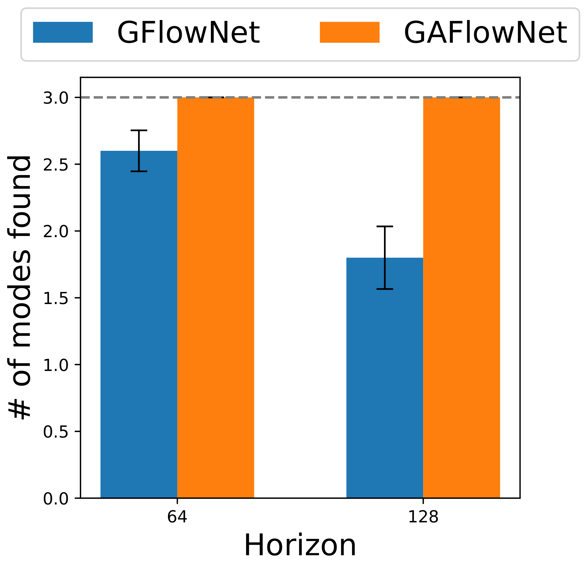
The potential difficulty in learning only from the terminal reward is related to the challenge of sparse rewards in RL, where most states do not provide an informative reward. We demonstrate the sparse reward problem for GFlowNets and reveal interesting findings based on the GridWorld task (as shown in Figure 4) with sparse rewards. Specifically, the agent only receives a reward of +1+1+1 only when it reaches one of the 333 goals located around the corners of the world (except the starting state corner) with size H×HH \times HH×H (with H∈{64,128}H \in \{64, 128\}H∈{64,128}), and the reward is 000 otherwise. A more detailed description of the task can be found in Section 5.1. We evaluate the number of modes discovered by the GFlowNet trained with TB, following [5]. As summarized in Figure 1, GFlowNet training can get trapped in a subset of the modes. Therefore, it remains a critical challenge for GFlowNets to efficiently learn when the reward signal is sparse and non-informative.
On the other hand, there has been recent progress with intrinsic motivation methods ([19, 20]) to improve exploration of RL algorithms, where the agent learns from both a sparse extrinsic reward and a dense intrinsic bonus at each step. Building on this, we aim to address the exploration challenge of GFlowNets by enabling intermediate rewards in GFlowNets and thus intrinsic rewards.
We now propose our learning framework, which is dubbed Generative Augmented Flow Network (GAFlowNet), to take intermediate rewards into consideration.
4.1 Edge-based intermediate reward augmentation
We start our derivation from the flow matching consistency constraint, to take advantage of the insights brought by the water flow metaphor as discussed in Section 2. By incorporating intermediate rewards r(st→st+1)r({\mathbf{s}}_t \to {\mathbf{s}}_{t+1})r(st→st+1) for transitions from states st{\mathbf{s}}_tst to st+1{\mathbf{s}}_{t+1}st+1 into the flow matching constraint, we obtain
by considering an extra flow r(st→st+1)r({\mathbf{s}}_t \to {\mathbf{s}}_{t+1})r(st→st+1) going out of the transition st→st+1{\mathbf{s}}_t \to {\mathbf{s}}_{t+1}st→st+1. Based on Eq. (1), we define the corresponding forward and backward policies
Combining these, we obtain the detailed balance objective with the incorporation of intermediate rewards as
Finally, we have our resulting edge-based reward augmented learning objective for trajectory balance as in Eq. (4) via a telescoping calculation upon Eq. (3), where x=sn{\mathbf{x}}= {\mathbf{s}}_nx=sn, and Z=∑st−1→str(st−1→st)+∑xR(x)Z=\sum_{{\mathbf{s}}_{t-1} \to {\mathbf{s}}_t} r({\mathbf{s}}_{t-1} \to {\mathbf{s}}_t) + \sum_{{\mathbf{x}}} R({\mathbf{x}})Z=∑st−1→str(st−1→st)+∑xR(x) is the augmented total flow.
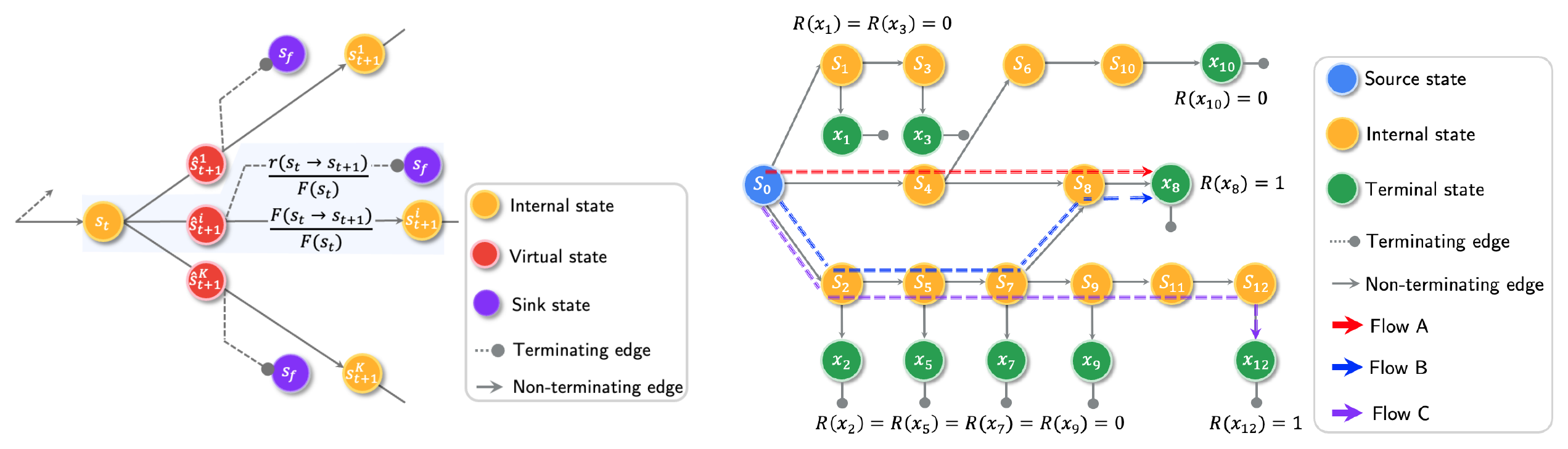
We explain the semantics of Eq. (4) in Figure 2(a). For the transition from an internal state (yellow circles) st{\mathbf{s}}_tst to the iii-th next state st+1i{\mathbf{s}}_{t+1}^ist+1i, we associate st+1i{\mathbf{s}}_{t+1}^ist+1i with a special state s^t+1i\hat{{\mathbf{s}}}_{t+1}^is^t+1i (red circle) with pseudo-exit. Specifically, from the state st{\mathbf{s}}_tst, we choose associated next states s^t+1\hat{{\mathbf{s}}}_{t+1}s^t+1 with probability (F(st→st+1)+r(st→st+1))/F(st)\left(F({\mathbf{s}}_t \to {\mathbf{s}}_{t+1}) + r({\mathbf{s}}_t \to {\mathbf{s}}_{t+1})\right) / F({\mathbf{s}}_t)(F(st→st+1)+r(st→st+1))/F(st) according to the forward policy in Eq. (2). At the associated next state s^t+1\hat{{\mathbf{s}}}_{t+1}s^t+1, we "virtually" choose the sink state (purple circles) sf{\mathbf{s}}_fsf with probability r(st→st+1)/F(st)r({\mathbf{s}}_t \to {\mathbf{s}}_{t+1}) / {F({\mathbf{s}}_t)}r(st→st+1)/F(st), or we choose the next state st+1{\mathbf{s}}_{t+1}st+1 with probability F(st→st+1)/F(st)F({\mathbf{s}}_t \to {\mathbf{s}}_{t+1}) / F({\mathbf{s}}_t)F(st→st+1)/F(st). Adding them together and multiplying these probabilities by the incoming flow F(st)F({\mathbf{s}}_t)F(st), we have F(st→st+1)+r(st→st+1)F({\mathbf{s}}_t \to {\mathbf{s}}_{t+1}) + r({\mathbf{s}}_t \to {\mathbf{s}}_{t+1})F(st→st+1)+r(st→st+1). Therefore, considering all possible next states, we have the augmented flow consistency equation (incoming flow === outgoing flow) as in Eq. (1). The intermediate rewards r(st→st+1)r({\mathbf{s}}_t \to {\mathbf{s}}_{t+1})r(st→st+1) are similar to transitions into a pseudo-exit that is never taken but still attracts larger probabilities into its ancestors in the DAG. From the water analogy, it can be considered that the flow from st{\mathbf{s}}_tst to st+1{\mathbf{s}}_{t+1}st+1 (and thus the probability of choosing that transition) is augmented by all the intermediate rewards due to pseudo-exits in all the accessible downstream transitions.
In contrast to simply adding a constant uniform probability to every action (which is commonly used for exploration with GFlowNets), the pseudo-exit intermediate rewards have an effect that is not local. In addition, we can specify non-uniform intermediate rewards as intrinsic motivation r(st→st+1)r({\mathbf{s}}_t \to {\mathbf{s}}_{t+1})r(st→st+1) with novelty-based methods ([19, 20]) to better tackle exploration in sparse reward tasks. Although how to accurately measure the novelty degree remains an open problem, it has been shown that random network distillation (RND) ([20]) is a simple yet effective method for encouraging the agent to visit states of interest. We use the difference between the predicted features by a trainable state encoder and a random fixed state encoder as the intrinsic rewards based on RND, i.e., ∣∣ϕ(s)−ϕˉrandom(s)∣∣2||\phi({\mathbf{s}}) - \bar{\phi}_{random}({\mathbf{s}})||_2∣∣ϕ(s)−ϕˉrandom(s)∣∣2. The random distillation network is trained by minimizing such differences. Therefore, the novelty measure is generally smaller for more often seen states or similar states. The overall training procedure is shown in Algorithm 1 by substituting the augmented trajectory balance loss according to Eq. (4).
We now demonstrate the conceptual advantage of edge-based reward augmentation in Figure 2(b). It depicts a flow network Markov decision process (MDP) with sparse rewards, where only R(x8)R({\mathbf{x}}_8)R(x8) and R(x12)R({\mathbf{x}}_{12})R(x12) are 111 and other terminal rewards are all 000. Consider the case where the agent had already discovered solution x8{\mathbf{x}}_8x8 with the red flow A. Since the rewards of most other solutions are 000, it can easily get trapped in the mode of x8{\mathbf{x}}_8x8, and thus fails to discover other solutions. Nonetheless, our edge-based reward augmentation could motivate the agent to discover other paths (e.g., the blue flow B) to x8{\mathbf{x}}_8x8, which can be beneficial for the agent to discover other solutions (e.g., x12{\mathbf{x}}_{12}x12) subsequently.
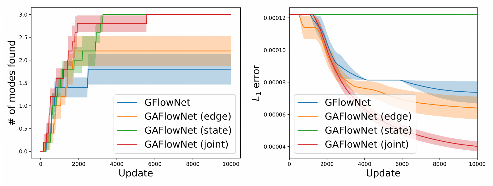
Following the evaluation scheme in ([5]), we summarize the number of discovered modes and the empirical L1L_1L1 error for GFlowNet and GAFlowNet with edge-based reward augmentation in Figure 3. The figure also includes the state-based and joint objectives introduced in later sections (Section 4.2 and Section 4.3) for completeness. The L1L_1L1 error is defined as E[∣p(x)−π(x)∣]\mathbb{E}\left[|p({\mathbf{x}}) - \pi({\mathbf{x}})|\right]E[∣p(x)−π(x)∣], where p(x)=R(x)/Zp({\mathbf{x}})={R({\mathbf{x}})}/{Z}p(x)=R(x)/Z denotes the true reward distribution, and we estimate π\piπ by repeated sampling and summarizing frequencies for visitation of each possible state x{\mathbf{x}}x. As shown, GAFlowNet (edge) is able to discover more modes as opposed to a standard GFlowNet and improves diversity. In addition, it learns more efficiently and leads to a smaller level of L1L_1L1 error.
4.2 State-based intermediate reward augmentation
Although the learning framework of edge-based reward augmentation is able to improve the diversity of solutions found, it still fails to discover all of the modes as shown in Figure 3. We hypothesize that this is due to its "local" exploration ability, where it is able to consider different paths to solution xi{\mathbf{x}}_ixi with non-zero rewards. However, it fails to sufficiently motivate the agent to globally explore solutions whose rewards may be zero. Therefore, it can still get trapped in a few modes, lacking sufficient exploration ability to discover other modes.
Different from the edge-based reward augmentation, [1] defines a trajectory return as the sum of intermediate rewards in a state-based reward augmentation manner. Specifically, state-based reward augmentation for trajectory balance yields the following criterion
and we also use RND for intrinsic rewards. Such an objective directly motivates the agent to explore different terminate states in a more global way (e.g., x2{\mathbf{x}}_2x2, x5{\mathbf{x}}_5x5, x7{\mathbf{x}}_7x7, x9{\mathbf{x}}_9x9 in Figure 2(b), which are beneficial for discovering x12{\mathbf{x}}_{12}x12). As shown in Figure 3(a), it is able to discover all the modes, exhibiting great diversity. However, it explicitly changes the underlying target probability distribution, and is directly and highly affected by the length of the trajectory. Therefore, this leads to much slower convergence as demonstrated in Figure 3(b).
4.3 Joint intermediate reward augmentation
As discussed above, the state-based reward augmentation is effective in improving diversity but fails to fit the target distribution efficiently. On the other hand, edge-based reward augmentation performs more efficiently, but lacks sufficient exploration ability which cannot discover all the modes.
Therefore, we propose a joint method to take both state and edge-based intermediate reward augmentation into account to reap the best from both worlds. Specifically, we redefine the trajectory return as the sum of the terminal reward and the intrinsic reward for the terminal state only. This can be considered as we augment the extrinsic terminal reward with its curiosity degree. On the other hand, we include intrinsic rewards for internal states according to the edge-based reward augmentation. This integration inherits the merits of both state and edge-based reward augmentation, which makes it possible to improve exploration in a more global way while learning more efficiently.
Our resulting flow consistency constraint is shown in Eq. (6) where ZZZ is the augmented total flow ∑xR(x)+∑st−1→str(st−1→st)\sum_{{\mathbf{x}}} R({\mathbf{x}}) + \sum_{{\mathbf{s}}_{t-1} \to {\mathbf{s}}_t} r({\mathbf{s}}_{t-1} \to {\mathbf{s}}_t)∑xR(x)+∑st−1→str(st−1→st). Our new optimization objective LGAFlowNet(τ)\mathcal{L}_{GAFlowNet}(\tau)LGAFlowNet(τ) is Eq. (7) which is trained by Algorithm 1.
In Theorem 1, we theoretically justify that the resulting joint augmentation method leads to an unbiased solution to the original formulation asymptotically. The proof can be found in Appendix A. Note that we employ RND ([20]) for the intrinsic rewards, which decrease as the agent has more knowledge about the state.
Theorem 1
Suppose that ∀τ,LGAFlowNet(τ)=0\forall \tau, \mathcal{L}_{{GAFlowNet}}(\tau)=0∀τ,LGAFlowNet(τ)=0, and ∀x,R(x)+r(x)>0\forall {\mathbf{x}}, R({\mathbf{x}}) + r({\mathbf{x}}) > 0∀x,R(x)+r(x)>0. When edge-based intrinsic rewards converge to 000, we have that (1) P(x)=R(x)+r(x)∑x[R(x)+r(x)]P({\mathbf{x}}) = \frac{R({\mathbf{x}}) + r({\mathbf{x}})}{\sum_{{\mathbf{x}}} \left[R({\mathbf{x}}) + r({\mathbf{x}})\right]}P(x)=∑x[R(x)+r(x)]R(x)+r(x); (2) If state-based intrinsic rewards converge to 000, then P(x)P({\mathbf{x}})P(x) is an unbiased sample distribution.
As shown in Figure 3, the joint method is able to discover all of the modes. In addition, it converges to the smallest level of L1L_1L1 error, and is more efficient than state-based and edge-based formulations, which validates its effectiveness in practice.
5. Experiments
We conduct comprehensive experiments to understand the effectiveness of our method and investigate the following key questions: i) How does GAFlowNet compare against previous baselines? ii) What are the effects of state and edge-based flow augmentation, the form of the intrinsic reward mechanism, and critical hyperparameters? iii) Can it scale to larger-scale and more complex tasks?
5.1 GridWorld
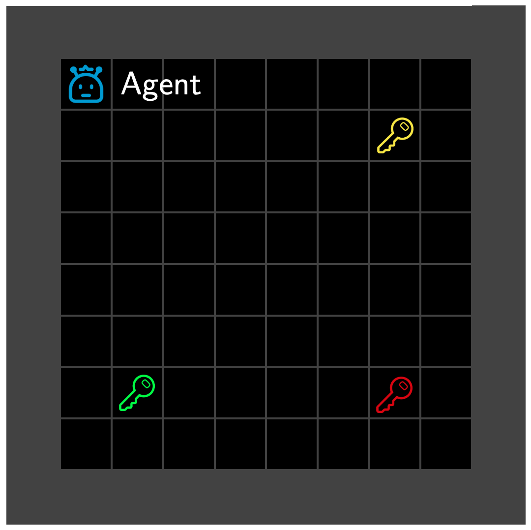
We first conduct a series of experiments based on GridWorld with sparse rewards (Figure 4). The task is the same as introduced in ([5]), except that the reward function is sparse as described in Section 4, which makes it much harder due to the challenge of exploration. With a larger value of the size HHH, it requires the agent to plan in a longer horizon and learn from sparse reward signals. Actions include operations to increase one coordinate as in ([5]), and a stop operation indicating termination to guarantee that the underlying MDP is a directed acyclic graph. We compare GAFlowNet against strong baselines including Metropolis-Hastings-MCMC ([22]), PPO ([23]), and a GFlowNet ([9]). We also include a variant of PPO with intrinsic rewards based on the same intrinsic motivation mechanism using RND ([20]). All baselines are implemented based on the open-source code1. Each algorithm is run for five random seeds, and we report their mean and standard deviation. A detailed description of the hyperparameters and setup can be found in Appendix B.1.
5.1.1 Performance Comparison
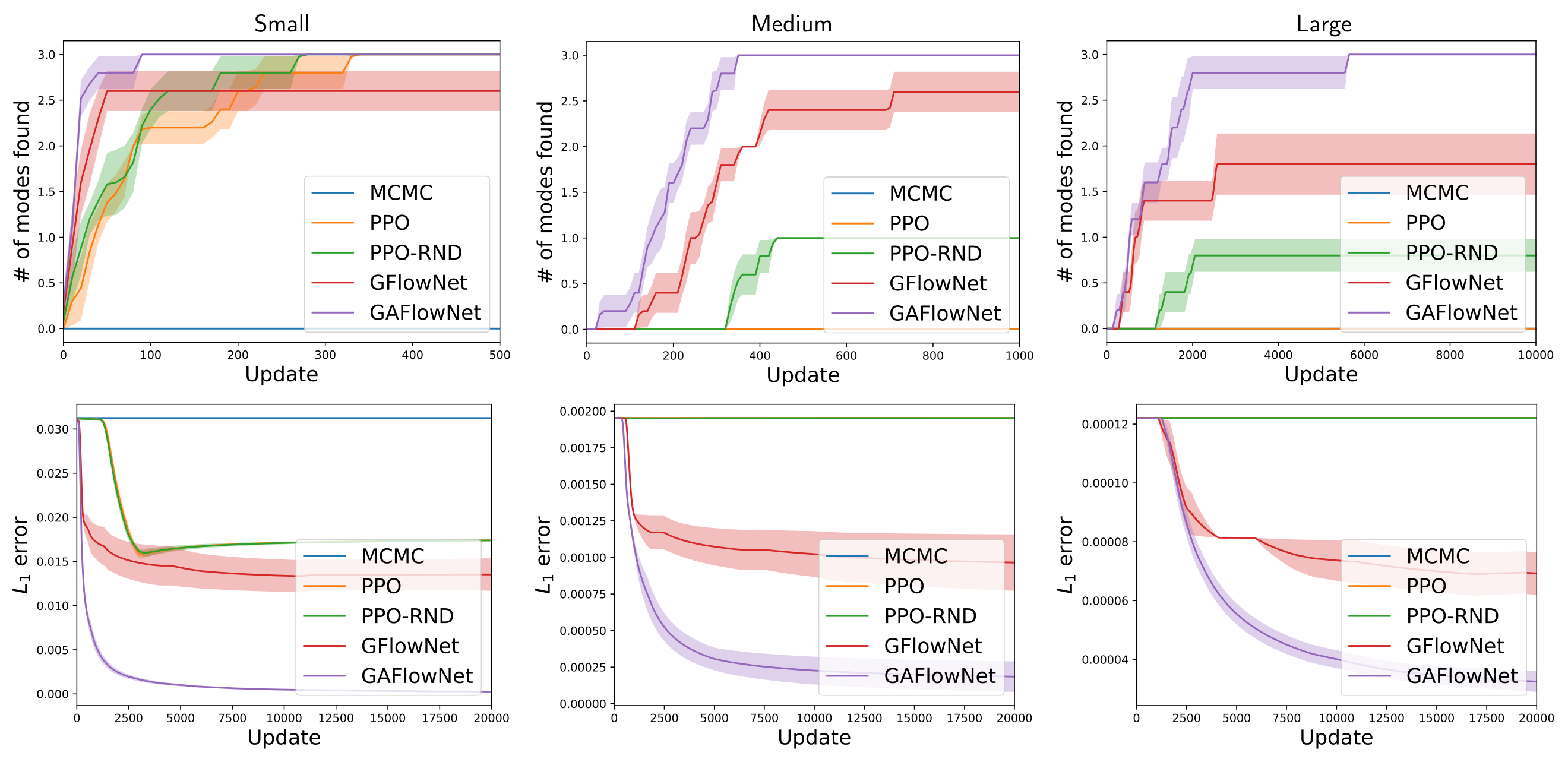
We conduct experiments on small, medium, and large GridWorlds with increasing sizes HHH. Full results of other values of HHH can be found in Appendix B.2. To investigate the effectiveness of GAFlowNet, we first compare it against baselines in terms of the empirical L1L_1L1 error as computed in Section 4. As shown in the first row in Figure 5, MCMC and PPO fail to converge due to the particularly sparse rewards. Although PPO-RND has a smaller L1L_1L1 error, it still underperforms GFlowNets by a large margin. GAFlowNet converges fastest and to the smallest level of L1L_1L1 error, which shows that our method is effective to both explore efficiently and converge to sampling goals with probability proportional to the extrinsic reward function even if the reward signals are sparse.
The number of modes that each method discovers during the course of training is shown in the second row in Figure 5. Although incorporating PPO with intrinsic rewards improves the number of discovered modes compared to that of PPO in larger-scale tasks, it still plateaus quickly. On the other hand, GFlowNets can get trapped in a few modes, while GAFlowNet is able to discover all of the modes efficiently. A detailed comparison in terms of performance can be found in Appendix B.3.
5.1.2 Ablation Study
We now provide an in-depth ablation study on the important components and hyperparameters of GAFlowNet in the large GridWorld task. We also study the effect of different mechanisms of intrinsic rewards besides RND, where results can be found in Appendix B.4.
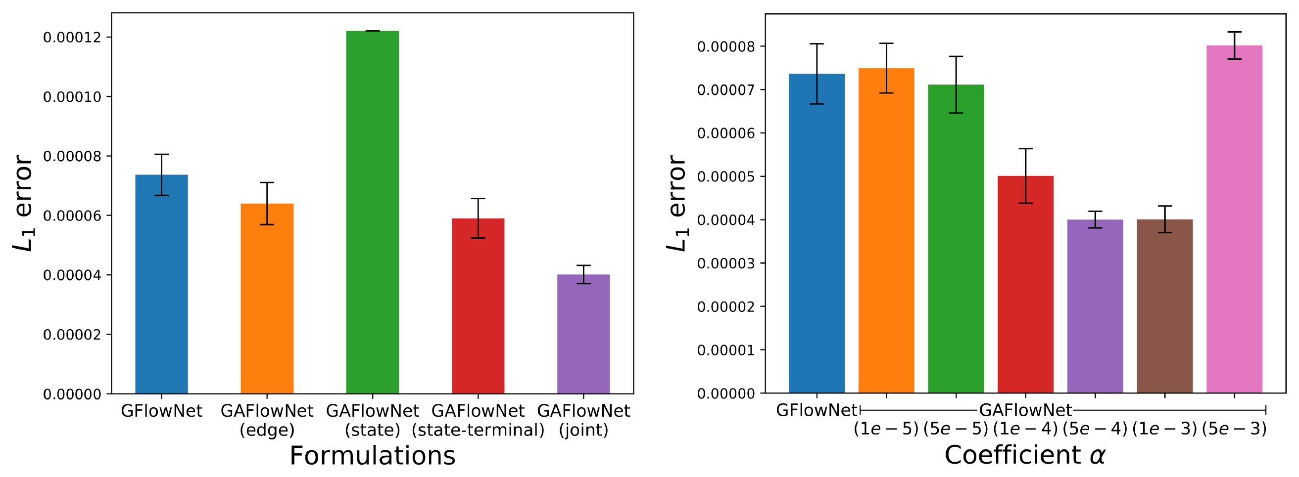
The effect of state-based and edge-based flow augmentation. In Figure 6(a), we investigate the effect of edge-based, state-based, and joint intrinsic rewards. As discussed in Section 4, incorporating intrinsic rewards for the trajectory in a state-based manner can result in slower convergence, which has a large L1L_1L1 error. On the other hand, augmenting the TB objective with intrinsic rewards in an edge-based way still fails to motivate the agent to visit states with zero rewards. In contrast, the joint augmentation mechanism is effective in both diversity and performance, achieving the smallest level of L1L_1L1 error in our experiments. It is also worth noting that only incorporating the intrinsic reward for the terminal state using state-based augmentation is less efficient, which implies the importance of both edge-based and terminal state-based intrinsic rewards.
The effect of the coefficient of intrinsic rewards. In practice, we scale intrinsic rewards by a coefficient. Figure 6(b) illustrates the effect of the coefficient of the intrinsic rewards. A too small coefficient does not improve the performance, while a too large coefficient converges slower. There exists an intermediate value that provides the best trade off.
5.1.3 Versatility
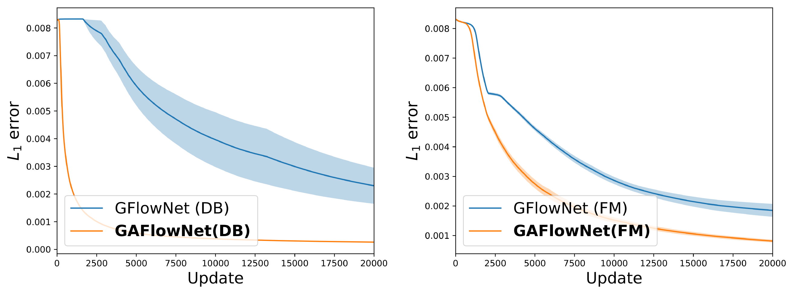
We now demonstrate that our proposed framework is versatile by building it upon the other two GFlowNet objectives based on the detailed balance (DB) ([1]) and flow matching (FM) ([5]) criteria. Comparison of empirical L1L_1L1 error averaged over increasing sizes HHH are summarized in Figure 7. As demonstrated, GAFlowNet also significantly improves training convergence of DB and FM, which provides consistent improvement gains.
5.2 Molecule Generation
5.2.1 Experimental Setup
We now investigate the effectiveness of our method in larger-scale tasks, by evaluating it on the more challenging molecule generation task ([5]) as depicted in Figure 8(a). A molecule is represented by a graph, which consists of a vocabulary of building blocks. The agent sequentially generates the molecule by choosing where to attach a block and also which block to attach at each step considering chemical validity constraints. There is also an exit action indicating whether the agent decides to stop the generation process. This problem is challenging with large state (about 101610^{16}1016) and action (around 100100100 to 200020002000) spaces. The agent aims to discover diverse molecules with high rewards, i.e., low binding energy to the soluble epoxide hydrolase (sEH) protein. We use a pretrained proxy model to compute this binding energy. We consider a sparse reward function here, where the agent only obtains a non-zero reward if the corresponding molecule succeeds to meet a target score, and the reward is 000 otherwise. A detailed description of the environment is in Appendix B.1.1. We compare our method with previous GFlowNet results ([5]), PPO ([23]), PPO with intrinsic rewards based on RND, and MARS ([24]). All baselines are implemented based on the open-source code2 and run with three random seeds as in ([5]). More details for the setup can be found in Appendix B.1.2.
5.2.2 Performance Comparison
We follow the evaluation metric in ([5]) and investigate our method in both performance and diversity. Figure 8(b) demonstrates the average reward of the top-101010 unique molecules generated by each method. The number of modes discovered by each method with rewards above 7.57.57.5 is summarized in Figure 8(c). We compute the average pairwise Tanimoto similarities for the top-101010 samples in Figure 8(d). Additional comparison results can be found in Appendix B.5.

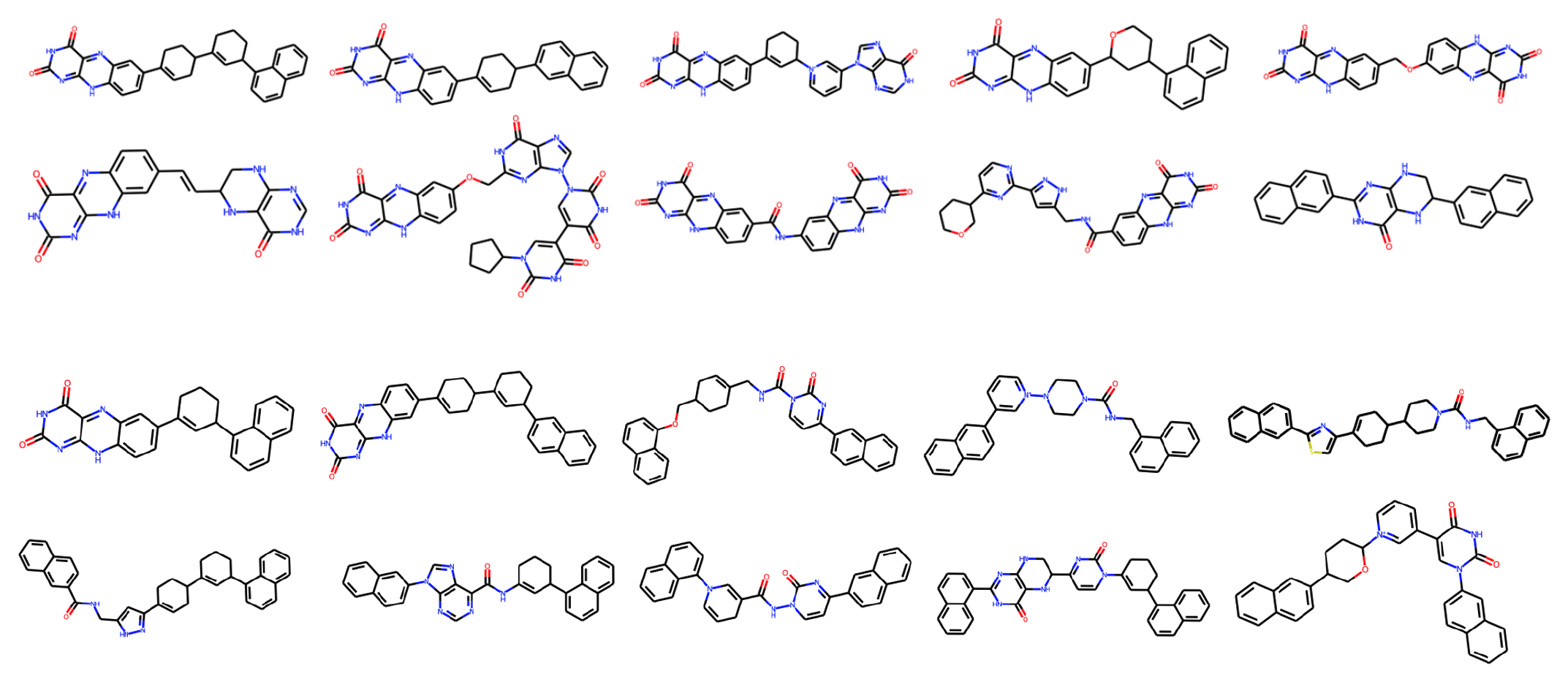
As shown, MARS fails to perform well given sparse rewards since most of the reward signals are non-informative. On the other hand, PPO and its variant with intrinsic rewards are better at finding higher-quality solutions than MARS, but suffer both from high similarities of the samples. The unaugmented GFlowNet is better at discovering more diverse molecules, but does not perform well in terms of solution quality. GAFlowNet significantly outperforms baseline methods in performance and diversity. We also visualize the top-101010 molecules generated by GFlowNet and GAFlowNet in a run in Figure 9. As shown, GAFlowNet is able to generate diverse and high-quality molecules efficiently, which demonstrates consistent and significant performance improvement.

6. Conclusion
In this paper, we propose a new learning framework, GAFlowNet, for GFlowNet to incorporate intermediate rewards. We specify intermediate rewards by intrinsic motivation to tackle the exploration problem of GFlowNets in sparse reward tasks, where it can get trapped in a few modes. We conduct extensive experiments to evaluate the effectiveness of GAFlowNets, which significantly outperforms strong baselines in terms of diversity, convergence, and performance when the rewards are very sparse. GAFlowNet is also scalable to complex tasks like molecular graph generation.
Reproducibility Statement
All details for our experiments are in Appendix B with a detailed description of the task, hyperparameters, network architectures for baselines, and setup. Our implementation for all baselines and environments is based on open-source repositories. The proof of Theorem 1 can be found in Appendix A. The code will be open-sourced upon publication of the work.
Appendix
A. Proof of Theorem 1
Theorem 1. Suppose that ∀τ,LGAFlowNet(τ)=0\forall \tau, \mathcal{L}_{{GAFlowNet}}(\tau)=0∀τ,LGAFlowNet(τ)=0, and ∀x,R(x)+r(x)>0\forall {\mathbf{x}}, R({\mathbf{x}}) + r({\mathbf{x}}) > 0∀x,R(x)+r(x)>0. When edge-based intrinsic rewards converge to 000, we have that (1) P(x)=R(x)+r(x)∑x[R(x)+r(x)]P({\mathbf{x}}) = \frac{R({\mathbf{x}}) + r({\mathbf{x}})}{\sum_{{\mathbf{x}}} \left[R({\mathbf{x}}) + r({\mathbf{x}})\right]}P(x)=∑x[R(x)+r(x)]R(x)+r(x); (2) If state-based intrinsic rewards converge to 000, then P(x)P({\mathbf{x}})P(x) is an unbiased sample distribution.
Proof: By definition, we have that
Since ∀τ,LGAFlowNet(τ)=0\forall \tau, \mathcal{L}_{{GAFlowNet}}(\tau)=0∀τ,LGAFlowNet(τ)=0, we have that
Therefore, we obtain that
When edge-based intrinsic rewards converge to 000 and FFF does not vanish, we have that
Due to the law of total probability, we have that
Therefore, Pθ(x)=R(x)+r(x)ZP_{\theta}({\mathbf{x}}) = \frac{R({\mathbf{x}}) + r({\mathbf{x}})}{Z}Pθ(x)=ZR(x)+r(x). As ∑xPθ(x)=1\sum_x P_{\theta}({\mathbf{x}}) = 1∑xPθ(x)=1, we also get that Z=∑x(R(x)+r(x))Z = \sum_{{\mathbf{x}}} \left(R({\mathbf{x}}) + r({\mathbf{x}})\right)Z=∑x(R(x)+r(x)).
Therefore, we have Part (1) that
Based on the above analysis, P(x)P({\mathbf{x}})P(x) is an unbiased estimation when state-based intrinsic rewards converge to 000, and we have Part (2).
B. Experimental Details
B.1 Experimental Setup
B.1.1 Task
The molecule generation task We adopt a pretrained proxy model for the reward, which is trained on a dataset of 300,000300, 000300,000 molecules that are randomly generated as provided in ([5]). For the original dense reward function, the agent receives a reward based on the normalized score. Here, we use a sparse reward function, where the agent only obtains the original non-zero reward if the normalized score succeeds to meet a target score (7.07.07.0), and the reward is 000 otherwise. As described in Section 5.2.1, the agent can choose one of the blocks to attach from the basic building blocks vocabulary (with a size of 105105105).
B.1.2 Baseline
All baseline methods are implemented based on the open-source implementation as described in the main text, where we follow the default hyperparameters and setup as in ([5]). Specifically, in GridWorld, the GFlowNet model is a feedforward network consisting of two hidden layers with 256256256 hidden units per layer using LeakyReLU activation. We train all models based on samples from a parallel of 161616 rollouts in the environment. We leverage random network distillation (RND) ([20]) as the intrinsic reward mechanism, where the random target network and the predictor network are both feedforward networks consisting of two hidden layers with 256256256 hidden units per layer using LeakyReLU activation. We train the GFlowNet model and RND jointly based on the Adam ([25]) optimizer with a learning rate of 0.0010.0010.001 for the policy models (PFP_FPF and PBP_BPB) and 0.10.10.1 for ZZZ. For the molecule generation task, we use a reward proxy provided in ([5]). As the molecule is represented as an atom graph, we use Message Passing Neural Networks (MPNN) ([26]) as the network architecture for all models. Note that we build our method upon GFlowNet based on the flow matching criterion in the molecule generation task, since it is the most competitive version in this task in terms of finding high-quality and diverse candidates. For GAFlowNet, the only hyperparameter that requires tuning is the coefficient α\alphaα of intrinsic rewards, where we use a same value for state-based and edge-based augmentation. We tune α\alphaα in {0.001,0.005,0.01,0.05,0.1,0.5}\{0.001, 0.005, 0.01, 0.05, 0.1, 0.5\}{0.001,0.005,0.01,0.05,0.1,0.5} with grid search. Specifically, α=0.001\alpha=0.001α=0.001 for GridWorld with all values of horizon except for H=64H=64H=64, where we set α\alphaα to be 0.0050.0050.005. For the molecule generation task, α\alphaα is set to be 0.10.10.1. The code will be released upon publication of the paper.
B.2 Full results in GridWorld
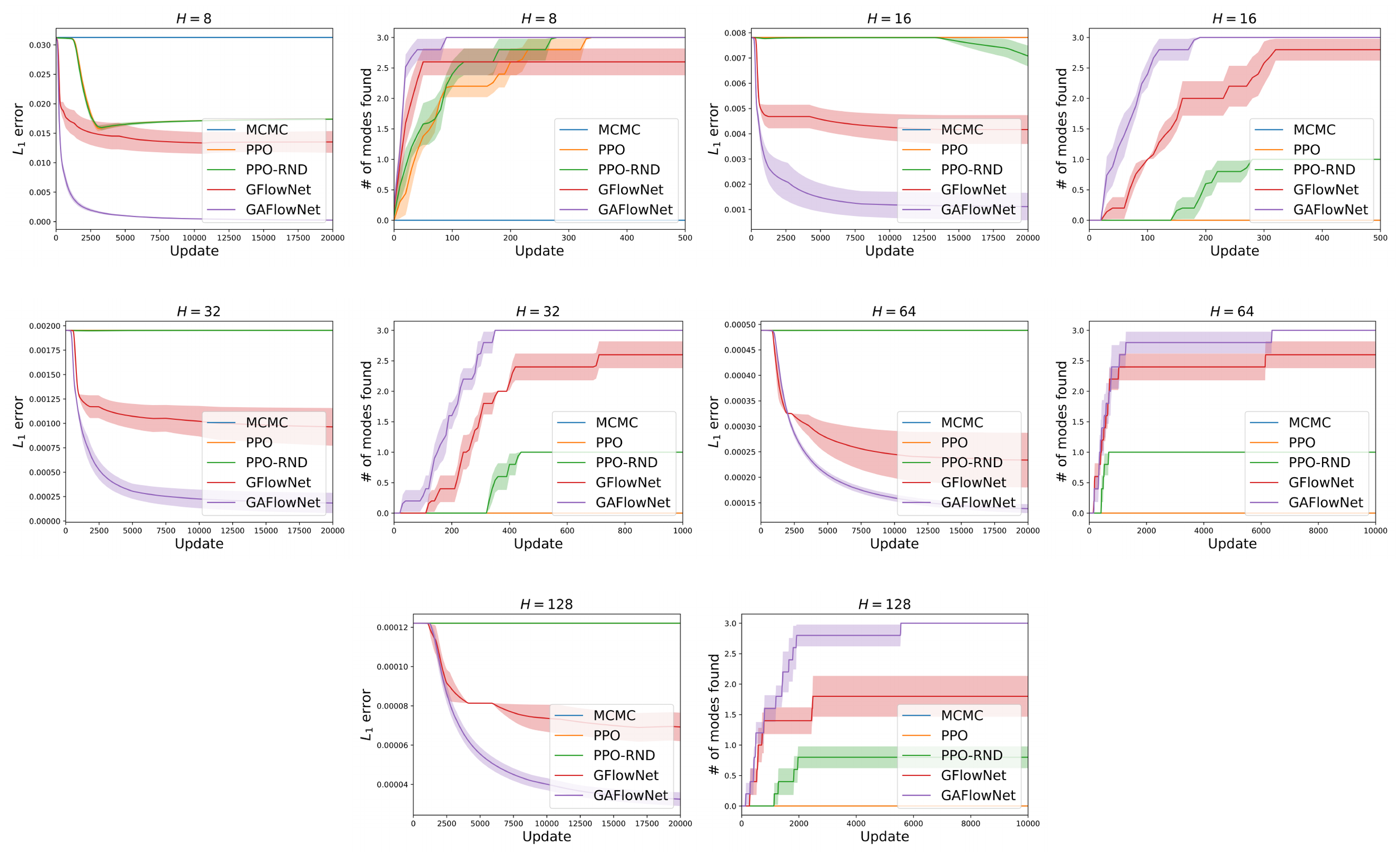
We show in Figure 10 the full comparison results in GridWorld with increasing sizes H{8,16,32,64,128}H \{8, 16, 32, 64, 128\}H{8,16,32,64,128}. As shown, GAFlowNet significantly outperforms baselines in empirical L1L_1L1 error and the number of modes found.
B.3 Performance comparison
Apart from evaluating our method based on the metrics (the number of modes discovered by each method and empirical L1L_1L1 error) as in ([5]), we are also interested in its performance after each update. Here, we evaluate the performance of baselines after each update (instead of throughout the training process) as in the evaluation scheme of RL algorithms. Figure 11 demonstrates the performance for the top-555 solutions among a batch of 161616 parallel rollouts of each method after each update for GridWorld with sizes H∈{8,16,32,64,128}H \in \{8, 16, 32,64, 128\}H∈{8,16,32,64,128}. As shown, although PPO is more efficient than PPO, both of them underperform GFlowNet by a large margin (especially with a larger value of HHH). We find that GAFlowNet significantly outperforms baseline methods, and also performs more efficiently than GFlowNet.

B.4 Additional Ablation Study of GAFlowNet
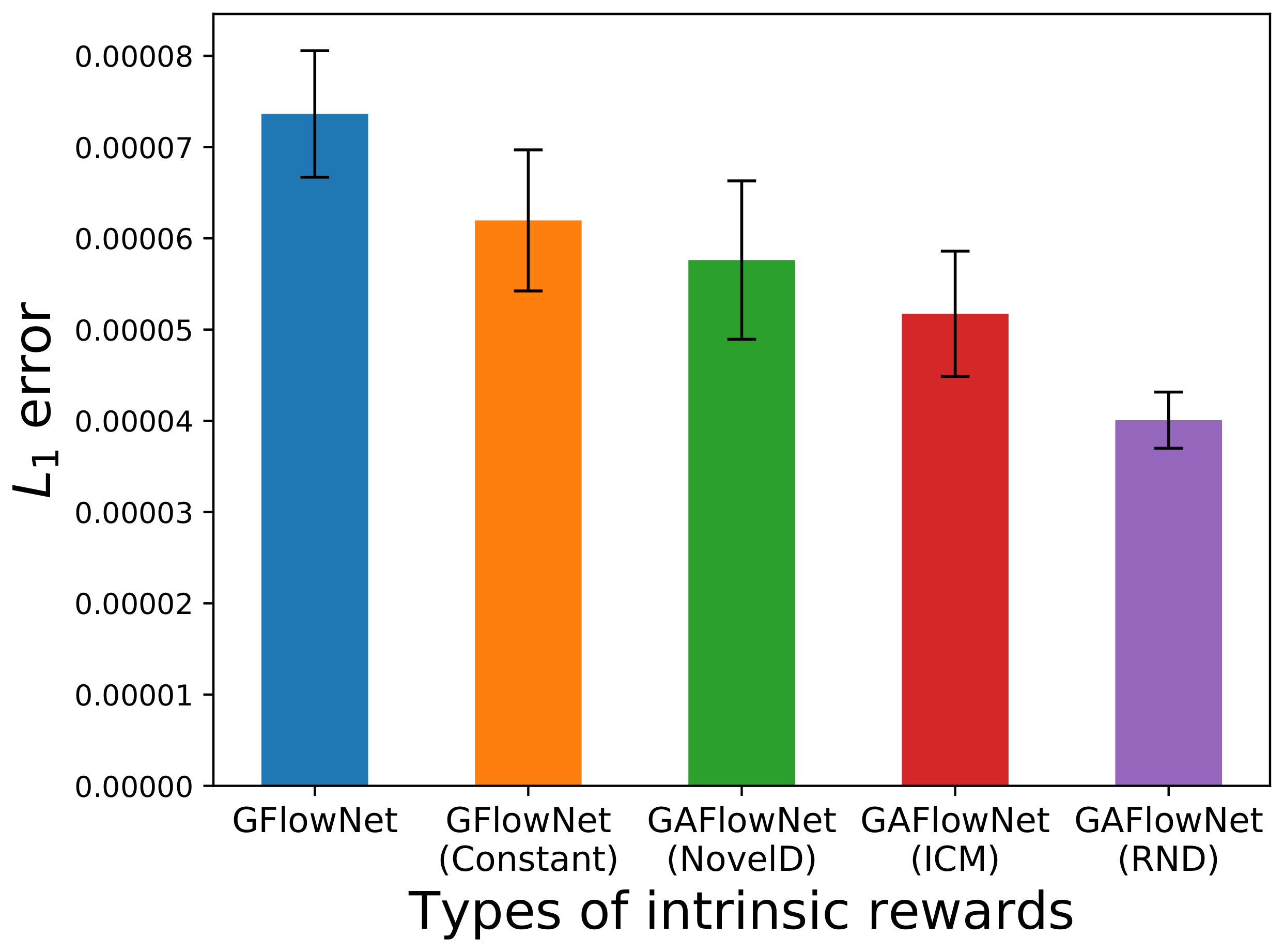
We investigate the effect of different types of intrinsic rewards including Intrinsic Curiosity Module (ICM) ([19]), Novelty Difference (NovelD) ([21]), and Random Network Distillation (RND) ([20]) in Figure 12, with fine-tuned coefficients for intrinsic rewards. We also include a baseline with constant intrinsic rewards in GAFlowNet, which mimics the behavior of ϵ\epsilonϵ-greedy exploration typically used in reinforcement learning algorithms. As demonstrated, GAFlowNet is not sensitive to the forms of intrinsic rewards, but RND enables the fastest convergence in our simulations. It also validates the effectiveness of the novelty-based methods from the comparison of GAFlowNet and GAFlowNet with constant intrinsic rewards. This is because novelty-based methods are more efficient than blindly wandering in the maze.
B.5 Additional Performance Comparison on the Molecule Generation Task
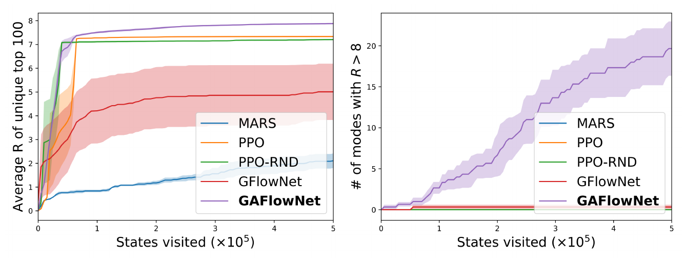
Following the evaluation metrics in ([5]), besides the results in Figure 8 in the main text, we also evaluate the average reward of the top-100100100 molecules and the number of modes with R>8.0R>8.0R>8.0 discovered by each method. As demonstrated in Figure 13, GAFlowNet achieves consistent and significant performance improvement over previous baselines.
B.6 Full visualization of top-101010 molecules
Figure 14 demonstrates the top-101010 molecules generated by GFlowNet and GAFlowNet, where GAFlowNet discovers more diverse and higher-quality solutions.
References
[1] Yoshua Bengio, Tristan Deleu, Edward J Hu, Salem Lahlou, Mo Tiwari, and Emmanuel Bengio. Gflownet foundations. arXiv preprint arXiv:2111.09266, 2021b.
[2] Volodymyr Mnih, Koray Kavukcuoglu, David Silver, Andrei A Rusu, Joel Veness, Marc G Bellemare, Alex Graves, Martin Riedmiller, Andreas K Fidjeland, Georg Ostrovski, et al. Human-level control through deep reinforcement learning. Nature, 518(7540):529–533, 2015.
[3] David Silver, Aja Huang, Chris J Maddison, Arthur Guez, Laurent Sifre, George Van Den Driessche, Julian Schrittwieser, Ioannis Antonoglou, Veda Panneershelvam, Marc Lanctot, et al. Mastering the game of go with deep neural networks and tree search. Nature, 529(7587):484–489, 2016.
[4] Oriol Vinyals, Igor Babuschkin, Wojciech M Czarnecki, Michaël Mathieu, Andrew Dudzik, Junyoung Chung, David H Choi, Richard Powell, Timo Ewalds, Petko Georgiev, et al. Grandmaster level in starcraft ii using multi-agent reinforcement learning. Nature, 575(7782):350–354, 2019.
[5] Emmanuel Bengio, Moksh Jain, Maksym Korablyov, Doina Precup, and Yoshua Bengio. Flow network based generative models for non-iterative diverse candidate generation. Advances in Neural Information Processing Systems, 34:27381–27394, 2021a.
[6] Moksh Jain, Emmanuel Bengio, Alex Hernandez-Garcia, Jarrid Rector-Brooks, Bonaventure FP Dossou, Chanakya Ajit Ekbote, Jie Fu, Tianyu Zhang, Michael Kilgour, Dinghuai Zhang, et al. Biological sequence design with gflownets. In International Conference on Machine Learning, pages 9786–9801. PMLR, 2022b.
[7] Matevž Kunaver and Tomaž Požrl. Diversity in recommender systems–a survey. Knowledge-based systems, 123:154–162, 2017.
[8] Yichi Zhang, Zhijian Ou, and Zhou Yu. Task-oriented dialog systems that consider multiple appropriate responses under the same context. In Proceedings of the AAAI Conference on Artificial Intelligence, volume 34, pages 9604–9611, 2020.
[9] Nikolay Malkin, Moksh Jain, Emmanuel Bengio, Chen Sun, and Yoshua Bengio. Trajectory balance: Improved credit assignment in gflownets. arXiv preprint arXiv:2201.13259, 2022.
[10] David Silver, Satinder Singh, Doina Precup, and Richard S Sutton. Reward is enough. Artificial Intelligence, 299:103535, 2021.
[11] Dinghuai Zhang, Ricky T. Q. Chen, Nikolay Malkin, and Yoshua Bengio. Unifying generative models with gflownets. 2022a.
[12] Dinghuai Zhang, Nikolay Malkin, Z. Liu, Alexandra Volokhova, Aaron C. Courville, and Yoshua Bengio. Generative flow networks for discrete probabilistic modeling. In ICML, 2022b.
[13] Tristan Deleu, Ant'onio G'ois, Chris C. Emezue, Mansi Rankawat, Simon Lacoste-Julien, Stefan Bauer, and Yoshua Bengio. Bayesian structure learning with generative flow networks. ArXiv, abs/2202.13903, 2022.
[14] Moksh Jain, Emmanuel Bengio, Alex García, Jarrid Rector-Brooks, Bonaventure F. P. Dossou, Chanakya Ajit Ekbote, Jie Fu, Tianyu Zhang, Micheal Kilgour, Dinghuai Zhang, Lena Simine, Payel Das, and Yoshua Bengio. Biological sequence design with gflownets. In ICML, 2022a.
[15] Hagai Attias. Planning by probabilistic inference. In AISTATS, 2003.
[16] Brian D. Ziebart. Modeling purposeful adaptive behavior with the principle of maximum causal entropy. 2010.
[17] Tuomas Haarnoja, Haoran Tang, Pieter Abbeel, and Sergey Levine. Reinforcement learning with deep energy-based policies. In International conference on machine learning, pages 1352–1361. PMLR, 2017.
[18] Tuomas Haarnoja, Aurick Zhou, Pieter Abbeel, and Sergey Levine. Soft actor-critic: Off-policy maximum entropy deep reinforcement learning with a stochastic actor. In International conference on machine learning, pages 1861–1870. PMLR, 2018.
[19] Deepak Pathak, Pulkit Agrawal, Alexei A Efros, and Trevor Darrell. Curiosity-driven exploration by self-supervised prediction. In International conference on machine learning, pages 2778–2787. PMLR, 2017.
[20] Yuri Burda, Harrison Edwards, Amos Storkey, and Oleg Klimov. Exploration by random network distillation. In International Conference on Learning Representations, 2018.
[21] Tianjun Zhang, Huazhe Xu, Xiaolong Wang, Yi Wu, Kurt Keutzer, Joseph E Gonzalez, and Yuandong Tian. Noveld: A simple yet effective exploration criterion. Advances in Neural Information Processing Systems, 34:25217–25230, 2021.
[22] Hanjun Dai, Rishabh Singh, Bo Dai, Charles Sutton, and Dale Schuurmans. Learning discrete energy-based models via auxiliary-variable local exploration. Advances in Neural Information Processing Systems, 33:10443–10455, 2020.
[23] John Schulman, Filip Wolski, Prafulla Dhariwal, Alec Radford, and Oleg Klimov. Proximal policy optimization algorithms. arXiv preprint arXiv:1707.06347, 2017.
[24] Yutong Xie, Chence Shi, Hao Zhou, Yuwei Yang, Weinan Zhang, Yong Yu, and Lei Li. Mars: Markov molecular sampling for multi-objective drug discovery. In International Conference on Learning Representations, 2020.
[25] Diederik P Kingma and Jimmy Ba. Adam: A method for stochastic optimization. arXiv preprint arXiv:1412.6980, 2014.
[26] Justin Gilmer, Samuel S Schoenholz, Patrick F Riley, Oriol Vinyals, and George E Dahl. Neural message passing for quantum chemistry. In International conference on machine learning, pages 1263–1272. PMLR, 2017.