Activation-Space Uncertainty Quantification for Pretrained Networks

Richard BergnaStefan DepewegSergio Calvo OrdoñezJonathan PlenkÁlvaro CarteaJose Miguel Hernández-Lobato

article2026arXiv1 citations

Introduces Gaussian Process Activations, a post-hoc method that enables single-pass, closed-form uncertainty quantification for pretrained vision and language models while strictly preserving their original predictions without retraining or sampling.

Listen

Deploying modern pre-trained deep neural networks in risk-sensitive domains requires reliable uncertainty estimation so that systems know when they are likely to be wrong or encountering unfamiliar data. However, existing uncertainty quantification techniques often require costly model retraining, multiple forward passes at test time, or computationally expensive second-order calculations that do not scale well to modern large-scale architectures. Many existing post-hoc methods also alter the base model’s original predictions or struggle when output dimensions become very large.

The article introduces and evaluates Gaussian Process Activations (GAPA), a post-hoc framework designed to provide reliable, single-pass uncertainty estimates for frozen, pre-trained neural networks without altering their baseline point predictions. The objective is to demonstrate that shifting uncertainty modeling from the model's weights to its internal hidden activation space can yield accurate epistemic uncertainty and out-of-distribution detection with minimal computational overhead.

The proposed approach replaces standard deterministic activation functions with Gaussian process modules whose posterior mean exactly matches the original activation function, guaranteeing that the pre-trained network's base outputs remain completely unchanged. To ensure high scalability, GAPA caches training-set activations during a single offline pass, compresses them into representative summary points using clustering techniques, and retrieves only a small local neighborhood of nearest points during evaluation. Uncertainty is then propagated forward analytically through the network layers in a single pass using closed-form variance rules, completely avoiding Monte Carlo sampling, backpropagation, and curvature matrix inversions. The authors evaluate this approach across regression tasks, image classification on standard vision benchmarks, biomedical image segmentation, and large language modeling.

The key findings indicate that GAPA consistently delivers high-quality uncertainty estimates with fast inference speeds. Across regression benchmarks, GAPA achieved the lowest negative log-likelihood and best quantile calibration compared to established baselines. In image classification, GAPA achieved top-tier out-of-distribution detection performance (for instance, an out-of-distribution area under the ROC curve of 0.953 on ResNet-56) while matching the baseline classifier's accuracy and executing in just 3.30 seconds—drastically faster than competitive Bayesian alternatives that require hundreds to thousands of seconds. In large language modeling experiments on LLaMA-3.2-3B, GAPA successfully separated in-distribution from shifted text distributions, outperforming global logit-scaling bounds and conventional last-layer methods.

These results demonstrate that reliable uncertainty quantification can be integrated into high-stakes production pipelines without incurring prohibitive latency, compute costs, or prediction drift. Organizations can safeguard deployment reliability and detect unfamiliar operational environments across diverse modalities without modifying or re-tuning frozen base models.

Moving forward, practitioners should consider activation-space uncertainty modeling as a scalable alternative to sampling-based ensembles or complex weight-space Bayesian methods, selecting moderate inducing points (such as k-means compression) and local neighborhood sizes to balance accuracy with memory. The primary limitation of the method is the memory required to store the cached activation index for large architectures. Additional work is recommended to explore hierarchical indexing schemes and structured inter-neuron dependencies to further reduce storage requirements while maintaining high uncertainty fidelity.

Department of Engineering Mathematical Institute Siemens AG University of Cambridge University of Oxford backpropagation algorithm bayesian methods classification Activation-Space Uncertainty Quantification predictive uncertainty epistemic uncertainty

arXiv: 2602.14934

Paper: A Simple Approach to Improve Single-Model Deep Uncertainty via Distance-Awareness, Jeremiah Zhe Liu et al. (2023). Read this first to understand the distance-aware Gaussian-process approach to single-model uncertainty that GAPA’s activation-space design contrasts with and seeks to scale.

No sufficiently relevant recommendations were found.

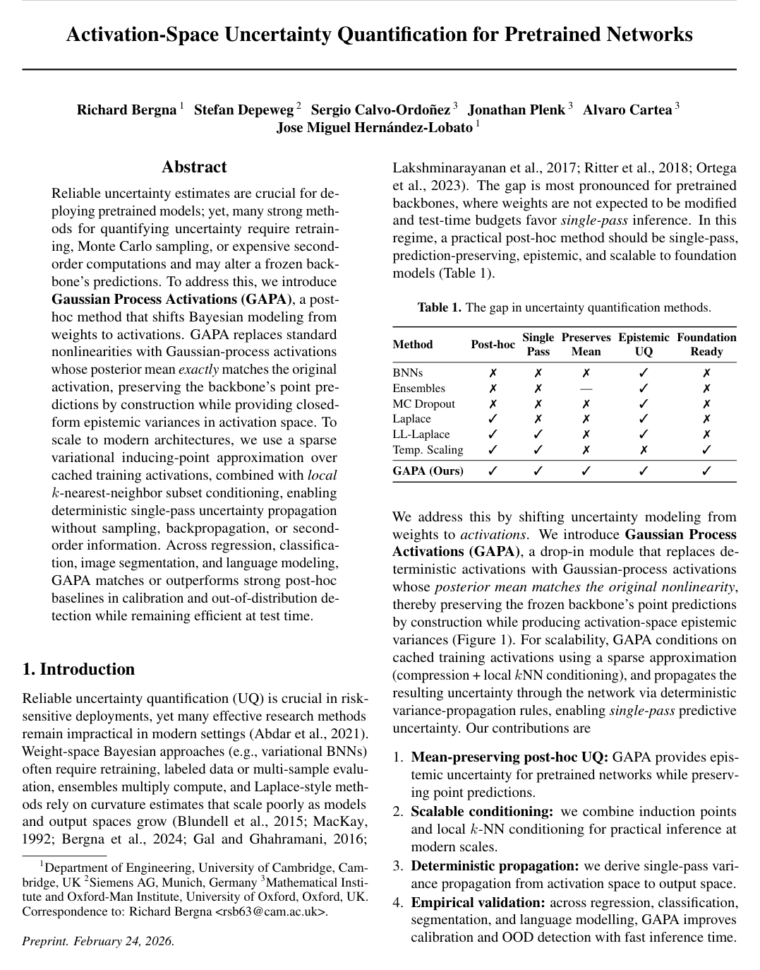
Cover for Activation-Space Uncertainty Quantification for Pretrained Networks

Abstract

Reliable uncertainty estimates are crucial for deploying pretrained models; yet, many strong methods for quantifying uncertainty require retraining, Monte Carlo sampling, or expensive second-order computations and may alter a frozen backbone's predictions. To address this, we introduce Gaussian Process Activations (GAPA), a post-hoc method that shifts Bayesian modeling from weights to activations. GAPA replaces standard nonlinearities with Gaussian-process activations whose posterior mean exactly matches the original activation, preserving the backbone's point predictions by construction while providing closed-form epistemic variances in activation space. To scale to modern architectures, we use a sparse variational inducing-point approximation over cached training activations, combined with local k-nearest-neighbor subset conditioning, enabling deterministic single-pass uncertainty propagation without sampling, backpropagation, or second-order information. Across regression, classification, image segmentation, and language modeling, GAPA matches or outperforms strong post-hoc baselines in calibration and out-of-distribution detection while remaining efficient at test time.

Topics

backpropagation algorithm bayesian methods classification closed-form expression deterministic gaussian processes gaussians image segmentation k-nearest neighbors language model

Keywords

Activation-Space Uncertainty Quantification predictive uncertainty epistemic uncertainty Gaussian-process activations post-hoc uncertainty variance propagation GP conditioning single-pass inference layer covariance

1 Introduction
2 Model Proposition
2.1 Uncertainty Modeling Perspective
2.2 Gaussian Process Activation Function
2.3 Local Inducing-Point Approximation
2.4 Variance Propagation Through the Network
2.5 Hyperparameter Strategy
3 Results
3.1 Regression
3.2 Classification
3.3 Language models
4 Related Work
5 Conclusion
References
A Conservativeness of Subset GP Conditioning
B Variational Inducing-Point Interpretation and Zero-Noise Limit
C Derivation for Stacking GAPA Layers
D ResNets Pretrained Neural Networks
E Image Segmentation
F LLaMA-3.2 Additional Results
G GAPA Hyperparameters
G.1 GAPA Empirical Hyperparameters
G.2 Regression Training Details
H Nearest–Neighbour Retrieval with Faiss
H.1 Index construction
H.2 Query procedure
H.3 Complexity
I Laplace-Bridge Approximation for Classification
J Metrics
J.1 Regression Metrics
J.2 Classification Metrics
K Variance Propagation in Transformer Architectures
K.1 Attention
K.2 RMSNorm
K.3 Softmax
L Tables with Standard Deviations
L.1 Regression
L.2 Feedforward Neural Network Classification
L.3 ResNet
M Ablation Studies
M.1 Where to put GAPA
M.2 Number of inducing inputs
M.3 Inducing point selection: KMeans vs. farthest-point sampling
M.4 Random vs Furthers Point Sampling
M.5 KNN Sweep: K=1K=1 to 500500
N Extended Related Work

Knowls

Knowl 1 — Mean-preserving Gaussian-process activations
model/method
Gaussian Process Activations (GAPA) adds uncertainty to a frozen neural network by replacing an element-wise activation function with a Gaussian-process (GP) activation, while leaving the network weights unchanged. At a selected layer of width $d$ , let $z\in\mathbb{R}^d$ be the pre-activation and let $\phi$ be the original element-wise activation. GAPA assigns the GP prior mean $m(z)=\phi(z)$ and conditions on cached pre-activations $\tilde z^{(m)}$ with pseudo-targets $\tilde y^{(m)}=\phi(\tilde z^{(m)})$ . Because the targets equal the prior mean at every cached input, the residuals in the GP posterior-mean update are zero, so the posterior mean is $\mu(z)=\phi(z)$ for every query $z$ . Replacing the original activation with this GP therefore preserves the frozen network’s deterministic point predictions, while its posterior covariance supplies activation-space epistemic uncertainty.
Knowl 2 — Diagonal activation-space posterior variance
equation
GAPA models each output neuron’s activation as an independent scalar GP, giving a diagonal layer covariance. For neuron $i$ , let $k_i$ be its kernel, let $Z_i$ be the set of conditioning pre-activations, let $K_i$ be the kernel matrix on $Z_i$ , let $k_i(z)$ be the vector of kernel values between query pre-activation $z$ and points in $Z_i$ , and let $\sigma_n^2>0$ be a small numerical-stability jitter. The posterior variance is
$\sigma_i^2(z)=k_i(z,z)-k_i(z)^\top(K_i+\sigma_n^2 I)^{-1}k_i(z).$
The layer covariance is $\Sigma(z)=\operatorname{diag}(\sigma_1^2(z),\ldots,\sigma_d^2(z))$ . This diagonal approximation treats neuron outputs as conditionally independent; it avoids storing and propagating dense $d\times d$ covariances. The variance is the GP’s activation-space epistemic signal, while the posterior mean remains the original activation.
Knowl 3 — Sparse cache and local inducing-point conditioning
model/method
GAPA makes activation-space GP inference practical by compressing cached training pre-activations and conditioning locally at test time. A single offline forward pass through the frozen network collects pre-activations; for a cache of $N$ points at a layer, $k$ -means can reduce them to $M\ll N$ inducing points. For each test pre-activation $z\in\mathbb{R}^d$ , approximate nearest-neighbour search retrieves the $K$ closest inducing points in Euclidean activation space, and the GP conditional-variance calculation is restricted to this local subset. The paper uses $K=50$ as its default. This replaces a solve over the full cache with a $K\times K$ solve: the reported per-query cost is $O(\log M)+O(K^3)$ , with approximate FAISS search and fixed $K$ making dependence on cache size sublinear in practice. With fixed kernel hyperparameters and observation noise, conditioning on a subset cannot reduce posterior variance relative to conditioning on the full inducing set; the local approximation can therefore inflate, but not underestimate, variance relative to that full-set GP. The paper also studies farthest-first inducing-point selection as an alternative to $k$ -means.
Knowl 4 — Deterministic variance propagation through frozen layers
equation
GAPA propagates a Gaussian summary—mean and diagonal variance—through the frozen network without sampling intermediate activations. For a linear layer $z=Wh+b$ , with input variance vector $v_h$ , the output variance vector is $v_z=(W\odot W)v_h$ , where $\odot$ denotes element-wise multiplication. For an element-wise nonlinearity $y=\phi(z)$ , first-order delta-method propagation uses $\mu_y\approx\phi(\mu_z)$ and $v_y\approx(\phi'(\mu_z))^{\odot 2}\odot v_z$ . At a downstream GAPA activation, the neuron-wise variance also includes the local GP epistemic variance and the correction for its uncertain input:
$\operatorname{Var}(y_i)\approx \sigma_{\mathrm{epi},i}^2(\mu_z)+\bigl(\phi'(\mu_{z,i})\bigr)^2v_{z,i}+\sigma_{y,i}^2.$
Here $\sigma_{\mathrm{epi},i}^2(\mu_z)$ is the local GP conditional variance evaluated at the input mean, $v_{z,i}$ is the incoming variance for neuron $i$ , and $\sigma_{y,i}^2$ is optional observation noise (set to zero for classification). Because the GP mean equals $\phi$ , this propagation preserves deterministic mean predictions while carrying uncertainty forward. The regression experiments add a learned heteroscedastic noise component.
Knowl 5 — Task-agnostic kernel settings and regression noise head
model/method
GAPA fixes its GP hyperparameters from cached activation statistics rather than optimizing them with a task-specific objective. The paper uses an RBF kernel, $k_i(z,z')=\sigma_{k,i}^2\exp(-\|z-z'\|_2^2/(2\ell_i^2))$ : the length scale is set to the empirical median of pairwise distances between cached training inputs, approximated from $10^6$ sampled pairs, and the neuron-specific signal scale is set from the standard deviation of that neuron’s training pre-activations, with a minimum of $10^{-6}$ . Inducing points are selected with $k$ -means or, in the alternative procedure studied, farthest-first traversal. For regression, the paper additionally trains only a small noise head $s_\psi$ ; the frozen backbone supplies the unchanged mean $\mu(x)$ , while the head sets $\sigma_{\mathrm{ale}}^2(x)=\operatorname{softplus}(s_\psi(x))+10^{-6}$ . The total predictive variance is the GAPA epistemic variance plus this aleatoric variance, and the noise-head parameters $\psi$ are fit by Gaussian negative log-likelihood. Thus the general attachment is post-hoc, but the reported regression setup includes this separate noise-head fitting.
Knowl 6 — Converting logit moments to classification probabilities
equation
For classification, let $\mu_c$ and $v_c$ be the propagated mean and variance of the logit for class $c$ , among $C$ classes. GAPA converts these moments into approximate predictive probabilities with the Laplace-bridge approximation:
$p(y=c\mid x)\approx\frac{\exp\!\left(\mu_c/\sqrt{1+(\pi/8)v_c}\right)}{\sum_{c'=1}^{C}\exp\!\left(\mu_{c'}/\sqrt{1+(\pi/8)v_{c'}}\right)}.$
The adjustment is applied element-wise before softmax and approximates integrating Gaussian logit uncertainty without sampling. Predictive entropy and BALD are then used as uncertainty scores, including for out-of-distribution detection. Since the propagated logit means are those of the frozen backbone, the class predictions’ mean logits are preserved; the uncertainty-aware probability calculation can nevertheless change predictive probabilities and their calibration.
Knowl 7 — Regression benchmarks: best negative log-likelihood on all three datasets
empirical result
On YEAR Prediction MSD, Airline, and Taxi regression benchmarks, results averaged over five random seeds show that GAPA achieved the lowest negative log-likelihood (NLL) among the compared methods on every dataset. Its respective NLL, continuous ranked probability score (CRPS), and centered quantile metric (CQM) were: Airline, $4.946$ , $18.068$ , and $0.103$ ; YEAR, $3.470$ , $4.663$ , and $0.014$ ; Taxi, $3.112$ , $4.035$ , and $0.104$ . GAPA also had the lowest CRPS on Airline and YEAR, but not Taxi, where ELLA scored $3.680$ ; its CQM was best on YEAR and Taxi, while VaLLA-200 scored better on Airline with $0.098$ . The results support strong predictive-distribution fit overall, but show that GAPA does not dominate every metric on every dataset.
Knowl 8 — MNIST and Fashion-MNIST: calibration, OOD detection, and runtime
empirical result
On two-layer, 200-hidden-unit tanh MLPs trained on MNIST and Fashion-MNIST, GAPA retained the backbone’s accuracy while improving uncertainty-based out-of-distribution (OOD) detection over the deterministic backbone. For MNIST, GAPA-Diag achieved accuracy $0.978$ , NLL $0.073$ , ECE $0.016$ , entropy-based OOD AUROC $0.963$ , and BALD AUROC $0.976$ ; GAPA-Full achieved $0.978$ , $0.072$ , $0.013$ , $0.969$ , and $0.983$ , respectively. For Fashion-MNIST, GAPA-Diag achieved $0.859$ , $0.390$ , $0.009$ , $0.941$ , and $0.993$ , while GAPA-Full achieved $0.859$ , $0.388$ , $0.009$ , $0.990$ , and $0.997$ . The deterministic backbone’s corresponding entropy AUROCs were $0.919$ and $0.846$ . GAPA-Diag’s test time was $2.05$ seconds on each dataset, compared with $1.24$ seconds on MNIST and $1.20$ seconds on Fashion-MNIST for the backbone; GAPA-Full took $8.92$ and $8.91$ seconds. These experiments also found competitive NLL under increasing image-rotation shifts, with uncertainty increasing as inputs moved farther from the training distribution.
Knowl 9 — CIFAR-10 ResNets: strong OOD detection at low inference cost
empirical result
For pretrained CIFAR-10 ResNet-44 and ResNet-56 classifiers, evaluated with SVHN as the OOD dataset, GAPA achieved OOD AUROCs of $0.931$ and $0.953$ with test times of $2.85$ and $3.30$ seconds, respectively. Accuracy remained at the deterministic backbone’s reported values: $94.0\%$ for ResNet-44 and $94.4\%$ for ResNet-56. GAPA’s NLL was $0.230$ on both models. VaLLA achieved a higher OOD AUROC on ResNet-56 ( $0.960$ versus $0.953$ ), but required $363.8$ seconds of test time; on ResNet-44 it achieved $0.928$ AUROC with $272.9$ seconds of test time. Thus GAPA’s result is a favorable OOD-detection/inference-cost trade-off, not uniformly the highest OOD score or lowest NLL.
Knowl 10 — Language-model OOD scoring from propagated activation uncertainty
empirical result
The authors attached GAPA post-hoc to LLaMA-3.2-3B (hidden size $3072$ ), caching about $12$ million pre-activations from WikiText-103 training sequences of length $96$ . For language-model propagation, they used deterministic attention weights and propagated uncertainty through the values; they also supplied rules for transformer components including RMSNorm. At each position, output logit means and variances were used to draw $S=512$ Gaussian logit samples over the top $k=512$ tokens, without additional network evaluations. Total uncertainty was predictive entropy, aleatoric uncertainty was the mean sample entropy, and epistemic uncertainty was their difference. The evaluation classified WikiText-103 validation sequences as in-distribution and OpenWebText sequences as OOD, averaging uncertainty scores over sequence positions. At layer $27$ with $K=50$ local neighbours, epistemic-uncertainty AUROC exceeded the study’s test-tuned global logit-temperature oracle once the inducing-point count was about $10^3$ or higher; later layers generally performed better than middle layers, and random inducing-point selection underperformed $k$ -means. The authors caution that OpenWebText is likely not OOD for the pretrained LLaMA model itself, but is OOD relative to the evaluated method.
Knowl 11 — High-dimensional segmentation via a compressed embedding
empirical result
As a proof of concept for dense prediction, the authors applied GAPA to a pretrained U-Net for three-class Oxford-IIIT Pet segmentation, using images resized to $128\times128$ . GAPA was inserted at the $64$ -dimensional embedding at the network bottleneck, after pooling and projection; the mean-preserving, variance-augmented embedding was then passed through the unchanged decoder. Qualitative validation examples showed accurate masks and spatially localized epistemic-uncertainty maps that highlighted regions of segmentation error. The experiment demonstrates a way to obtain uncertainty for a high-dimensional segmentation output by applying the GP at a compact internal representation, rather than forming a posterior over the full pixelwise output.
Knowl 12 — Limitations of diagonal covariance and inducing-cache storage
limitation
GAPA’s scalable propagation relies on a diagonal covariance approximation, which omits structured dependencies between neurons; extending the method to capture those dependencies while remaining computationally practical is left for future work. The paper identifies storage of inducing activations as its primary limitation and suggests compressed or hierarchical indexing as possible remedies. For transformer propagation, the authors also report that variances can compound across layers, particularly when uncertainty is propagated through attention scores as well as queries, keys, and values; their implemented attention rule therefore treats attention weights as deterministic and propagates variance through the values.

Coverage note — Detailed numerical ablations over inducing-set size, neighbour count, layer placement, and inducing-point selection are omitted to prioritize the central method and primary task results; their broad trends are included where most consequential.

References

1.Moloud Abdar, Farhad Pourpanah, Sadiq Hussain, Dana Rezazadegan, Li Liu, Mohammad Ghavamzadeh, Paul Fieguth, Xiaochun Cao, Abbas Khosravi, U Rajendra Acharya, et al. A review of uncertainty quantification in deep learning: Techniques, applications and challenges. Information fusion, 76:243–297, 2021.
2.Guillaume Alain and Yoshua Bengio. Understanding intermediate layers using linear classifier probes. arXiv preprint arXiv:1610.01644, 2016.
3.Richard Bergna, Sergio Calvo-Ordonez, Felix L Opolka, Pietro Liò, and Jose Miguel Hernandez-Lobato. Uncertainty modeling in graph neural networks via stochastic differential equations. arXiv preprint arXiv:2408.16115, 2024.
4.Charles Blundell, Julien Cornebise, Koray Kavukcuoglu, and Daan Wierstra. Weight uncertainty in neural network. In International conference on machine learning, pages 1613–1622. PMLR, 2015.
5.Erik Daxberger, Agustinus Kristiadi, Alexander Immer, Runa Eschenhagen, Matthias Bauer, and Philipp Hennig. Laplace redux-effortless bayesian deep learning. Advances in neural information processing systems, 34:20089–20103, 2021.
6.Zhijie Deng, Feng Zhou, and Jun Zhu. Accelerated linearized Laplace approximation for Bayesian deep learning. Advances in Neural Information Processing Systems, 35:2695–2708, 2022.
7.Matthijs Douze, Alexandr Guzhva, Chengqi Deng, Jeff Johnson, Gergely Szilvasy, Pierre-Emmanuel Mazaré, Maria Lomeli, Lucas Hosseini, and Hervé Jégou. The faiss library. IEEE Transactions on Big Data, 2025.
8.Yarin Gal and Zoubin Ghahramani. Dropout as a bayesian approximation: Representing model uncertainty in deep learning. In international conference on machine learning, pages 1050–1059. PMLR, 2016.
9.Tilmann Gneiting and Adrian E Raftery. Strictly proper scoring rules, prediction, and estimation. Journal of the American statistical Association, 102(477):359–378, 2007.
10.Robert B Gramacy and Daniel W Apley. Local Gaussian process approximation for large computer experiments. Journal of Computational and Graphical Statistics, 24(2):561–578, 2015.
11.Chuan Guo, Geoff Pleiss, Yu Sun, and Kilian Q Weinberger. On calibration of modern neural networks. In International conference on machine learning, pages 1321–1330. PMLR, 2017.
12.James Harrison, John Willes, and Jasper Snoek. Variational Bayesian last layers. arXiv preprint arXiv:2404.11599, 2024.
13.Kaiming He, Xiangyu Zhang, Shaoqing Ren, and Jian Sun. Deep residual learning for image recognition. In Proceedings of the IEEE conference on computer vision and pattern recognition, pages 770–778, 2016.
14.James Hensman, Nicolo Fusi, and Neil D Lawrence. Gaussian processes for big data. arXiv preprint arXiv:1309.6835, 2013.
15.Neil Houlsby, Ferenc Huszár, Zoubin Ghahramani, and Máté Lengyel. Bayesian active learning for classification and preference learning. arXiv preprint arXiv:1112.5745, 2011.
16.Arthur Jacot, Franck Gabriel, and Clément Hongler. Neural tangent kernel: Convergence and generalization in neural networks. Advances in neural information processing systems, 31, 2018.
17.Balaji Lakshminarayanan, Alexander Pritzel, and Charles Blundell. Simple and scalable predictive uncertainty estimation using deep ensembles. Advances in neural information processing systems, 30, 2017.
18.Yann LeCun, Léon Bottou, Yoshua Bengio, and Patrick Haffner. Gradient-based learning applied to document recognition. Proceedings of the IEEE, 86(11):2278–2324, 2002.
19.Jaehoon Lee, Yasaman Bahri, Roman Novak, Samuel S Schoenholz, Jeffrey Pennington, and Jascha Sohl-Dickstein. Deep neural networks as Gaussian processes. arXiv preprint arXiv:1711.00165, 2017.
20.Jeremiah Liu, Zi Lin, Shreyas Padhy, Dustin Tran, Tania Bedrax Weiss, and Balaji Lakshminarayanan. Simple and principled uncertainty estimation with deterministic deep learning via distance awareness. Advances in neural information processing systems, 33:7498–7512, 2020.
21.David JC MacKay. A practical Bayesian framework for backpropagation networks. Neural computation, 4(3):448–472, 1992.
22.Wesley J Maddox, Pavel Izmailov, Timur Garipov, Dmitry P Vetrov, and Andrew Gordon Wilson. A simple baseline for bayesian uncertainty in deep learning. Advances in neural information processing systems, 32, 2019.
23.Andrew McHutchon and Carl Rasmussen. Gaussian process training with input noise. Advances in neural information processing systems, 24, 2011.
24.Jishnu Mukhoti, Andreas Kirsch, Joost Van Amersfoort, Philip HS Torr, and Yarin Gal. Deep deterministic uncertainty: A new simple baseline. In Proceedings of the IEEE/CVF Conference on Computer Vision and Pattern Recognition, pages 24384–24394, 2023.
25.Luis A Ortega, Simón Rodríguez Santana, and Daniel Hernández-Lobato. Variational linearized Laplace approximation for Bayesian deep learning. arXiv preprint arXiv:2302.12565, 2023.
26.Omkar M Parkhi, Andrea Vedaldi, Andrew Zisserman, and CV Jawahar. Cats and dogs. In 2012 IEEE conference on computer vision and pattern recognition, pages 3498–3505. IEEE, 2012.
27.Hippolyt Ritter, Aleksandar Botev, and David Barber. A scalable laplace approximation for neural networks. In 6th international conference on learning representations, ICLR 2018-conference track proceedings, volume 6. International Conference on Representation Learning, 2018.
28.Olaf Ronneberger, Philipp Fischer, and Thomas Brox. U-net: Convolutional networks for biomedical image segmentation. In Medical image computing and computer-assisted intervention–MICCAI 2015: 18th international conference, Munich, Germany, October 5-9, 2015, proceedings, part III 18, pages 234–241. Springer, 2015.
29.Hugh Salimbeni and Marc Deisenroth. Doubly stochastic variational inference for deep Gaussian processes. Advances in neural information processing systems, 30, 2017.
30.Michalis Titsias. Variational learning of inducing variables in sparse Gaussian processes. In Artificial intelligence and statistics, pages 567–574. PMLR, 2009.
31.Christopher Williams and Matthias Seeger. Using the nyström method to speed up kernel machines. Advances in neural information processing systems, 13, 2000.
32.Han Xiao, Kashif Rasul, and Roland Vollgraf. Fashion-mnist: a novel image dataset for benchmarking machine learning algorithms. arXiv preprint arXiv:1708.07747, 2017.

Citation

MLA

Bergna, R., et al. “Activation-Space Uncertainty Quantification for Pretrained Networks”. arXiv, 2026, http://arxiv.org/abs/2602.14934v2.

APA

Bergna, R., Depeweg, S., Calvo-Ordoñez, S., Plenk, J., Cartea, A., & Hernández-Lobato, J. M. (2026). Activation-Space Uncertainty Quantification for Pretrained Networks. arXiv. http://arxiv.org/abs/2602.14934v2

Chicago

Bergna, R., S. Depeweg, S. Calvo-Ordoñez, J. Plenk, A. Cartea, and J. M. Hernández-Lobato. 2026. “Activation-Space Uncertainty Quantification for Pretrained Networks”. arXiv. http://arxiv.org/abs/2602.14934v2.

Harvard

Bergna, R. et al. (2026) “Activation-Space Uncertainty Quantification for Pretrained Networks”, arXiv [Preprint]. Available at: http://arxiv.org/abs/2602.14934v2.

Vancouver

1. Bergna R, Depeweg S, Calvo-Ordoñez S, Plenk J, Cartea A, Hernández-Lobato JM (2026) Activation-Space Uncertainty Quantification for Pretrained Networks. arXiv

BibTeX

@article{bergna2026activation,
  title = {Activation-Space Uncertainty Quantification for Pretrained Networks},
  author = {Bergna, Richard and Depeweg, Stefan and Calvo-Ordoñez, Sergio and Plenk, Jonathan and Cartea, Alvaro and Hernández-Lobato, Jose Miguel},
  year = {2026},
  journal = {arXiv},
  url = {http://arxiv.org/abs/2602.14934v2},
  eprint = {2602.14934}
}

Metadata:arXiv

Access the Paper

This paper is available from its original source. Click below to access the PDF.

Open PDF

License: https://creativecommons.org/licenses/by/4.0/

Activation-Space Uncertainty Quantification for Pretrained Networks

Abstract

Topics

Keywords

Table of Contents

Knowls

Knowl 1 — Mean-preserving Gaussian-process activations

Knowl 2 — Diagonal activation-space posterior variance

Knowl 3 — Sparse cache and local inducing-point conditioning

Knowl 4 — Deterministic variance propagation through frozen layers

Knowl 5 — Task-agnostic kernel settings and regression noise head

Knowl 6 — Converting logit moments to classification probabilities

Knowl 7 — Regression benchmarks: best negative log-likelihood on all three datasets

Knowl 8 — MNIST and Fashion-MNIST: calibration, OOD detection, and runtime

Knowl 9 — CIFAR-10 ResNets: strong OOD detection at low inference cost

Knowl 10 — Language-model OOD scoring from propagated activation uncertainty

Knowl 11 — High-dimensional segmentation via a compressed embedding

Knowl 12 — Limitations of diagonal covariance and inducing-cache storage

References

Citation

BibTeX

Access the Paper