Image Representation Using 2D Gabor Wavelets

Tai-Sing Lee

article1996TPAMI1,869 citations

Establishes mathematical completeness conditions and tight frame bounds for 2D Gabor wavelets, demonstrating how biologically plausible visual cortex filters enable stable image reconstruction even from coarsely quantized neural responses.

Listen

Biological vision systems process high-resolution visual scenes using individual neurons that possess very limited precision. While neurophysiological studies have established that simple cells in the primary visual cortex can be modeled as two-dimensional Gabor filters, practical questions have persisted regarding how biological systems and artificial computer vision models allocate orientation, frequency, and spatial sampling budgets to achieve complete and stable image representations without loss of detail.

The article establishes mathematical completeness criteria for two-dimensional Gabor wavelets by extending one-dimensional wavelet frame theory to two dimensions. It evaluates the exact sampling conditions under which these non-orthogonal wavelets form a "tight frame"—a mathematical property ensuring that an image can be stably and accurately reconstructed through direct linear addition of wavelet responses.

The analysis combined theoretical derivations constrained by cortical neurophysiology (including elliptical receptive field aspect ratios and zero-mean admissibility requirements) with numerical calculations of frame bounds across various orientation, frequency, and spatial sampling lattices. The resulting models were validated through image reconstruction experiments comparing direct linear summation against iterative error-minimization reconstruction, including tests where filter response coefficients were severely quantized down to low-bit precisions.

The findings demonstrate three key insights. First, complete image representation requires relatively minimal sampling: as few as three orientations can guarantee completeness when using iterative reconstruction. Second, increasing sampling density—specifically utilizing 1.5-octave bandwidth wavelets with suboctave frequency scaling (two to three frequency steps per octave), eight to twenty orientations, and spatial spacing under 0.8 wavelengths—produces an almost tight frame that eliminates the need for complex, costly mathematical inversions. Third, this redundant, tight-frame oversampling allows high-resolution visual details to be preserved even when individual filter coefficients are degraded to coarse, low-bit precision (such as three to four bits).

These results demonstrate that the extensive oversampling observed in the mammalian visual cortex serves a critical operational role: it compensates for the coarse, noisy resolution of individual neurons by enabling robust coarse-coding and direct linear readout. For engineering and computer vision systems, this means that highly accurate image representations and texture segmentations can be designed using simple linear reconstruction architectures, reducing computational complexity and improving tolerance to hardware or transmission noise.

Developers and modelers of vision systems are advised to employ 1.5-octave bandwidth Gabor wavelets with fractional frequency dilation (two to three voices per octave) and at least eight orientations to achieve near-optimal reconstruction efficiency. While further empirical research is needed to explore cortical computations beyond early representation (such as scene segmentation and boundary grouping), there is high analytical and experimental confidence in these parameter thresholds for stable, low-precision visual encoding.

Carnegie Mellon University Center for the Neural Basis of Cognition computer vision computer vision applications daubechies 2D Gabor wavelets image representation wavelet transforms

Lee (1996).pdf

No sufficiently relevant recommendations were found.

Cover for Image Representation Using 2D Gabor Wavelets

Abstract

This paper extends to two dimensions the frame criterion developed by Daubechies for one-dimensional wavelets, and it computes the frame bounds for the particular case of 2D Gabor wavelets. Completeness criteria for 2D Gabor image representations are important because of their increasing role in many computer vision applications and also in modeling biological vision, since recent neurophysiological evidence from the visual cortex of mammalian brains suggests that the filter response profiles of the main class of linearly-responding cortical neurons (called simple cells) are best modeled as a family of self-similar 2D Gabor wavelets. We therefore derive the conditions under which a set of continuous 2D Gabor wavelets will provide a complete representation of any image, and we also find self-similar wavelet parameterizations which allow stable reconstruction by summation as though the wavelets formed an orthonormal basis. Approximating a “tight frame” generates redundancy which allows low-resolution neural responses to represent high-resolution images, as we illustrate by image reconstructions with severely quantized 2D Gabor coefficients.

1 INTRODUCTION
2 DERIVATION OF THE 2D GABOR WAVELETS
3 NONORTHOGONAL WAVELETS AND FRAMES
4 2D GENERALIZATION OF DAUBECHIES'S FRAME CRITERION
5 FRAME BOUNDS FOR FRACTIONALLY DILATED 2D WAVELETS
6 FRAME BOUNDS FOR VARIOUS SAMPLING SCHEMES
7 ILLUSTRATIVE EXPERIMENTAL RESULTS
8 CONCLUSION
ACKNOWLEDGMENTS
REFERENCES

Knowls

Knowl 1 — Admissible Family of 2D Gabor Wavelets
model/method
A family of continuous 2D Gabor wavelets modeling the receptive fields of simple cells in the visual cortex is derived under four neurophysiological and mathematical constraints:
1. The aspect ratio $\beta / \sigma$ of the elliptical Gaussian envelope is $2:1$ , where $\sigma$ and $\beta$ are the standard deviations along the minor and major axes, respectively.
2. The plane wave modulation propagates along the short axis of the elliptical Gaussian: $\xi_0 = \omega_0 \cos\theta$ and $\nu_0 = \omega_0 \sin\theta$ , where $\omega_0 = \sqrt{\xi_0^2 + \nu_0^2}$ is the radial center frequency in radians per unit length and $\theta$ is the filter orientation in radians.
3. The half-amplitude spatial frequency bandwidth $\phi$ (in octaves) sets $\sigma = \kappa / \omega_0$ , where $\kappa = \sqrt{2\ln 2} \left( \frac{2^\phi + 1}{2^\phi - 1} \right)$ For a bandwidth of $\phi = 1.0$ octave, $\kappa \approx \pi$ ; for $\phi = 1.5$ octaves, $\kappa \approx 2.5$ .
4. Wavelet admissibility requires zero DC response ( $\hat{\psi}(0,0) = 0$ ), accomplished by subtracting the DC component of the cosine term.
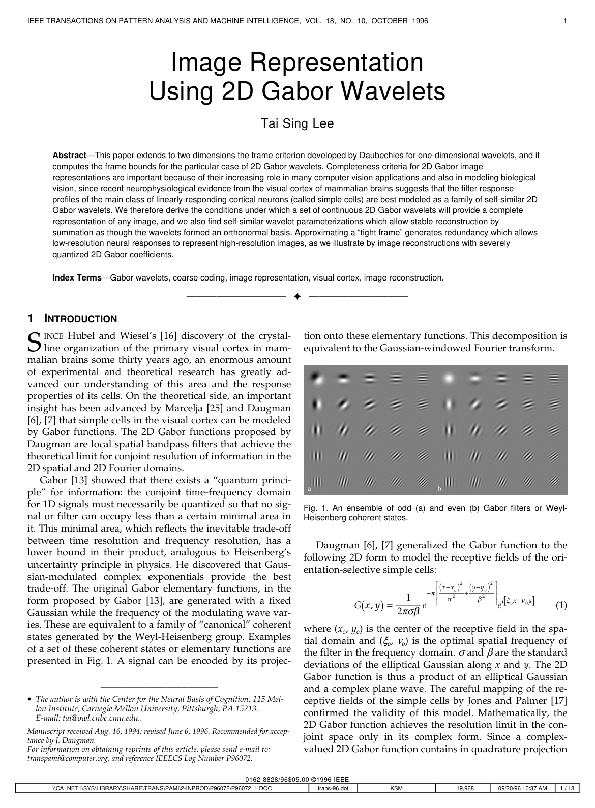
The resulting $L^2$ -normalized 2D Gabor wavelet centered at the origin is: $\psi(x, y, \omega_0, \theta) = \frac{\omega_0}{\sqrt{2\pi}\kappa} e^{-\frac{\omega_0^2}{8\kappa^2} \left( 4(x\cos\theta + y\sin\theta)^2 + (-x\sin\theta + y\cos\theta)^2 \right)} \left[ e^{i\omega_0(x\cos\theta + y\sin\theta)} - e^{-\frac{\kappa^2}{2}} \right]$

Its 2D Fourier transform is given by: $\hat{\psi}(\xi, \nu, \xi_0, \nu_0) = \frac{\sqrt{8\pi}\kappa}{\omega_0} \left[ e^{-\frac{2\kappa^2}{\omega_0^2} \left( [(\xi-\xi_0)\cos\theta + (\nu-\nu_0)\sin\theta]^2 + 4[-(\xi-\xi_0)\sin\theta + (\nu-\nu_0)\cos\theta]^2 \right)} - e^{-\frac{2\kappa^2}{\omega_0^2} \left( [\xi\cos\theta + \nu\sin\theta]^2 + 4[-\xi\sin\theta + \nu\cos\theta]^2 + \omega_0^2 \right)} \right]$

The entire family is generated by dilating and rotating the mother wavelet: $\psi(x,y) = \frac{1}{\sqrt{2\pi}} e^{-\frac{1}{8}(4x^2 + y^2)} \left[ e^{i\kappa x} - e^{-\frac{\kappa^2}{2}} \right]$ whose 2D Fourier transform is: $\hat{\psi}(\xi, \nu) = \sqrt{8\pi} \left[ e^{-\frac{1}{2}\left( (\xi-\kappa)^2 + 4\nu^2 \right)} - e^{-\frac{1}{2}\left( \xi^2 + 4\nu^2 + \kappa^2 \right)} \right]$
Knowl 2 — 2D Extension of Daubechies's Frame Criterion for Wavelet Representations
theoretical result
A discrete set of continuous 2D wavelets $\psi_{m,n,k,l}(x,y) = a_0^{-m} \psi_{\theta_l}(a_0^{-m}x - n b_0, a_0^{-m}y - k b_0)$ sampled at dilation step $a_0 > 1$ , orientation step $\theta_0 = \pi / K$ ( $l \in Q = \{0, 1, \dots, K-1\}$ ), and spatial translation steps $a_0^m b_0$ ( $m, n, k \in \mathbb{Z}$ ) constitutes a frame for $L^2(\mathbb{R}^2)$ with frame bounds $A > 0$ and $B < \infty$ if: $A \|f\|^2 \le \sum_{m,n,k,l} |\langle f, \psi_{m,n,k,l} \rangle|^2 \le B \|f\|^2$

For real-valued signals $f$ decomposed with complex 2D wavelets, the frame bounds are determined over the fundamental frequency sector $S = \{ (\xi, \nu) \in \mathbb{R}^2 \mid 1 \le \sqrt{\xi^2 + \nu^2} \le a_0, \, 0 \le \arctan(\nu / \xi) \le \pi / K \}$ : $A = \frac{1}{b_0^2} \left[ \inf_{(\xi,\nu) \in S} \sum_{m \in \mathbb{Z}, l \in Q} \frac{1}{2} \left( |\hat{\psi}_{\theta_l}(a_0^m\xi, a_0^m\nu)|^2 + |\hat{\psi}_{\theta_l}(-a_0^m\xi, -a_0^m\nu)|^2 \right) - R \right]$ $B = \frac{1}{b_0^2} \left[ \sup_{(\xi,\nu) \in S} \sum_{m \in \mathbb{Z}, l \in Q} \frac{1}{2} \left( |\hat{\psi}_{\theta_l}(a_0^m\xi, a_0^m\nu)|^2 + |\hat{\psi}_{\theta_l}(-a_0^m\xi, -a_0^m\nu)|^2 \right) + R \right]$

where the interference residue term $R$ is: $R = \sum_{\epsilon = \pm} \sum_{(p,q) \in \mathbb{Z}^2 \setminus \{(0,0)\}} \left[ \beta_\epsilon\left( \frac{2\pi p}{b_0}, \frac{2\pi q}{b_0} \right) \beta_\epsilon\left( -\frac{2\pi p}{b_0}, -\frac{2\pi q}{b_0} \right) \right]^{1/2}$ and the cross-product function $\beta_\epsilon(s,t)$ is defined as: $\beta_\epsilon(s,t) = \frac{1}{4} \sup_{(\xi,\nu) \in S} \sum_{m \in \mathbb{Z}, l \in Q} \left| \hat{\psi}_{\theta_l}(a_0^m\xi, a_0^m\nu) + \epsilon \hat{\psi}_{\theta_l}(-a_0^m\xi, -a_0^m\nu) \right| \cdot \left| \hat{\psi}_{\theta_l}(a_0^m\xi + s, a_0^m\nu + t) + \epsilon \hat{\psi}_{\theta_l}(-a_0^m\xi - s, -a_0^m\nu - t) \right|$
Knowl 3 — Frame Bounds for Multivoice Fractionally Dilated 2D Wavelets
theoretical result
When frequency space is sampled suboctavely with $N$ voices (frequency steps) per octave, the fractionally dilated 2D wavelets are defined by: $\psi^{\eta}(x, y) = 2^{-2\eta / N} \psi(2^{-\eta / N}x, 2^{-\eta / N}y), \quad \eta = 0, \dots, N-1$ with 2D Fourier transform $\hat{\psi}^\eta(\xi, \nu) = \hat{\psi}(2^{\eta/N}\xi, 2^{\eta/N}\nu)$ . The scaling parameter is $a_0 = 2$ , orientation step is $\theta_0 = \pi / K$ , and unit spatial translation step is $b_0$ .

For real signals represented by complex wavelets $\{\psi^{\eta}_{m,n,k,l}\}$ , the frame bounds are: $A = \frac{1}{b_0^2} \left[ \inf_{(\xi,\nu) \in S} \sum_{\eta=0}^{N-1} \sum_{m \in \mathbb{Z}, l \in Q} \frac{1}{2} \left( |\hat{\psi}^\eta_{\theta_l}(a_0^m\xi, a_0^m\nu)|^2 + |\hat{\psi}^\eta_{\theta_l}(-a_0^m\xi, -a_0^m\nu)|^2 \right) - R \right]$ $B = \frac{1}{b_0^2} \left[ \sup_{(\xi,\nu) \in S} \sum_{\eta=0}^{N-1} \sum_{m \in \mathbb{Z}, l \in Q} \frac{1}{2} \left( |\hat{\psi}^\eta_{\theta_l}(a_0^m\xi, a_0^m\nu)|^2 + |\hat{\psi}^\eta_{\theta_l}(-a_0^m\xi, -a_0^m\nu)|^2 \right) + R \right]$

where the cross-product residue term $R$ accounts for all $N$ suboctave voices: $R = \sum_{\epsilon = \pm} \sum_{\eta = 0}^{N-1} \sum_{(p,q) \in \mathbb{Z}^2 \setminus \{(0,0)\}} \left[ \beta_\epsilon^\eta\left( \frac{2\pi p}{b_0}, \frac{2\pi q}{b_0} \right) \beta_\epsilon^\eta\left( -\frac{2\pi p}{b_0}, -\frac{2\pi q}{b_0} \right) \right]^{1/2}$ and $\beta_\epsilon^\eta(s,t) = \frac{1}{4} \sup_{(\xi,\nu) \in S} \sum_{m \in \mathbb{Z}} \sum_{l=0}^{K-1} \left| \hat{\psi}^\eta_{\theta_l}(a_0^m\xi, a_0^m\nu) + \epsilon \hat{\psi}^\eta_{\theta_l}(-a_0^m\xi, -a_0^m\nu) \right| \cdot \left| \hat{\psi}^\eta_{\theta_l}(a_0^m\xi + s, a_0^m\nu + t) + \epsilon \hat{\psi}^\eta_{\theta_l}(-a_0^m\xi - s, -a_0^m\nu - t) \right|$

These wavelets form a valid frame ( $A > 0, B < \infty$ ) provided $b_0$ and $\theta_0$ are chosen small enough that $R$ is strictly smaller than the infimum of the principal spectral power sum.
Knowl 4 — Approximate Image Reconstruction via Linear Summation in Tight Gabor Frames
model/method
When a discrete family of 2D Gabor wavelets $\{\psi_{m,n,k,l}\}$ forms a tight or reasonably tight frame ( $B/A \approx 1$ ), an image $f(x,y)$ can be reconstructed directly by linear superposition using its own projection coefficients without requiring dual frame functions: $f_{\text{approx}}(x, y) = \frac{2}{A + B} \sum_{m,n,k,l} \langle f, \psi_{m,n,k,l} \rangle \psi_{m,n,k,l}(x, y)$

Here, $(A+B)/2$ represents the redundancy of the frame, and $B/A$ is the tightness ratio. In this formulation:
- The input image $f$ is projected onto the continuous wavelet functions via inner product $\langle f, \psi_{m,n,k,l} \rangle$ .
- As frame redundancy increases, the lower bound $A$ and upper bound $B$ increase and converge toward each other ( $B/A \to 1$ ), rendering the non-orthogonality cross-interference term negligible.
- When $B/A = 1$ (exact tight frame), this linear summation formula yields exact reconstruction, acting as an orthonormal basis expansion. When $B/A \approx 1$ , it provides a high-fidelity approximation.
Knowl 5 — Dual Frame Coefficient Estimation via Iterative Error Minimization
algorithm
When a 2D Gabor wavelet family forms a complete frame that is loose ( $B/A \gg 1$ ), direct linear summation introduces nonorthogonality artifacts. Exact reconstruction requires the projection coefficients $c_{m,n,k,l} = \langle f, \tilde{\psi}_{m,n,k,l} \rangle$ corresponding to the dual frame $\{\tilde{\psi}_{m,n,k,l}\}$ . These coefficients can be estimated iteratively by minimizing the squared reconstruction error functional $E$ .
Input: Image $f(x,y)$ , Gabor wavelet family $\{\psi_{m,n,k,l}(x,y)\}$ , step size $\mu$ , convergence threshold $\delta$
Output: Dual frame projection coefficients $c_{m,n,k,l}$
Initialize $c_{m,n,k,l} \leftarrow \langle f, \psi_{m,n,k,l} \rangle$ for all $m,n,k,l$
repeat
     $f_{\text{rec}}(x,y) \leftarrow \sum_{m,n,k,l} c_{m,n,k,l} \psi_{m,n,k,l}(x,y)$
     $e(x,y) \leftarrow f(x,y) - f_{\text{rec}}(x,y)$
     $E \leftarrow \iint |e(x,y)|^2 dx dy$
    for each index $(m,n,k,l)$ do
         $g_{m,n,k,l} \leftarrow -2 \iint e(x,y) \psi_{m,n,k,l}^*(x,y) dx dy$
         $c_{m,n,k,l} \leftarrow c_{m,n,k,l} - \mu \cdot g_{m,n,k,l}$
    end for
until $\Delta E < \delta$
return $c_{m,n,k,l}$
The image is subsequently synthesized as $f(x,y) = \sum_{m,n,k,l} c_{m,n,k,l} \psi_{m,n,k,l}(x,y)$ . If the wavelet family forms a complete frame, $E \to 0$ ; if the family is incomplete, residual error remains non-zero.
Knowl 6 — Phase-Space Sampling Constraints and Critical Bounds for 2D Gabor Frames
theoretical result
Because every 2D Gabor wavelet in the proposed family contains a line of zeros in the spatial frequency plane: $\xi \xi_0 + \nu \nu_0 = 0$ all wavelets sharing the same orientation $\theta$ share the exact same line of zeros where $\hat{\psi}(\xi, \nu) = 0$ . Consequently:
1. At least two distinct sampling orientations ( $K \ge 2$ ) are required to span the 2D frequency domain (except at the origin $(0,0)$ ). The critical orientation step $\theta_0^c$ is strictly upper bounded by: $\theta_0^c < \frac{\pi}{2}$
2. For single-voice sampling ( $N = 1$ ), the Nyquist criterion imposes a maximum spatial sampling interval $\Delta x \le \lambda / 2$ where $\lambda$ is the filter wavelength. Since $\Delta x = a_0 b_0$ with $a_0 = \sigma = \lambda / 2$ , the upper bound on the unit spatial translation step is $b_0^c \le 1$ . For multivoice fractionally dilated lattices ( $N > 1$ ), $b_0^c$ can exceed $1$ because fractional scales interleave onto denser combined spatial lattices.
3. The critical parameter bounds $b_0^c$ , $\theta_0^c$ , and $a_0^c$ mark the exact transition points where the lower frame bound $A$ becomes non-positive ( $A \le 0$ ), beyond which the wavelet set ceases to be a complete frame.

Knowl 7 — Frame Bounds and Tightness Ratios for 1.5-Octave Bandwidth 2D Gabor Wavelets

data/table

Numerical computation of the frame bounds $A$ and $B$ , together with the tightness ratio $B/A$ , demonstrates how frame tightness depends on the number of sampling orientations $K$ , suboctave voices $N$ , and spatial sampling interval $b_0 = \Delta x / a_0$ for 2D Gabor wavelets with a 1.5-octave bandwidth.

	$N = 1, b_0 = 0.8$			$N = 3, b_0 = 0.8$
$K$	$A$	$B$	$B/A$	$A$	$B$	$B/A$
4	2.502	54.388	21.739	19.273	136.424	7.079
6	17.131	56.965	3.325	67.908	144.066	2.122
8	32.107	62.141	1.935	118.664	161.044	1.357
12	57.150	81.810	1.432	201.665	217.529	1.079
16	78.494	107.516	1.370	272.766	286.155	1.049
20	98.499	134.178	1.362	341.454	357.199	1.046
	$N = 1, K = 20$			$N = 3, K = 20$
$b_0$	$A$	$B$	$B/A$	$A$	$B$	$B/A$
0.25	1087.822	1294.789	1.190	3576.876	3577.334	1.000
0.50	271.955	323.697	1.190	894.219	894.333	1.000
0.75	117.261	147.473	1.258	393.801	401.112	1.019
0.80	98.499	134.178	1.362	341.454	357.200	1.046
1.00	33.033	115.880	3.508	184.056	263.082	1.429
1.25	-	-	-	65.683	220.456	3.357

Key takeaways:

When $N=1$ , the frame cannot become perfectly tight ( $B/A$ plateaus around $1.19$ even as $b_0 \to 0$ ).
Adding suboctave voices ( $N=3$ ) enables near-perfect tightness ( $B/A = 1.000$ for $b_0 \le 0.50$ , and $B/A = 1.046$ for $K=20, b_0=0.80$ ).
For $N=1, b_0=1.25$ , the parameters fail to form a frame (denoted by '-').

Knowl 8 — Frame Bounds and Tightness Ratios for 1.0-Octave Bandwidth 2D Gabor Wavelets

data/table

Numerical computation of frame bounds $A, B$ and tightness ratio $B/A$ for 1.0-octave bandwidth 2D Gabor wavelets shows that narrower spectral bandwidth filters require denser sampling to achieve frame tightness compared to 1.5-octave filters.

	$N = 1, b_0 = 0.8$			$N = 3, b_0 = 0.8$
$K$	$A$	$B$	$B/A$	$A$	$B$	$B/A$
4	-	-	-	-	-	-
6	-	-	-	2.727	125.798	46.137
8	-	-	-	34.536	129.686	3.755
12	7.266	74.224	10.215	92.217	152.605	1.655
16	15.765	92.388	5.860	134.362	192.045	1.429
20	21.068	114.444	5.432	170.087	237.924	1.398
	$N = 1, K = 20$			$N = 3, K = 20$
$b_0$	$A$	$B$	$B/A$	$A$	$B$	$B/A$
0.25	543.289	844.349	1.554	2087.619	2090.410	1.001
0.50	135.817	211.093	1.554	521.899	522.608	1.001
0.75	39.490	114.692	2.904	210.553	253.672	1.205
0.80	21.067	114.444	5.432	170.087	237.924	1.399
1.00	-	-	-	57.254	203.873	3.561
1.25	-	-	-	1.550	165.572	106.846

Key takeaways:

The notation '-' indicates parameter combinations where $A \le 0$ , meaning the wavelets fail to form a frame.
For $N=1, b_0=0.8$ , $K \le 8$ does not form a frame; at $K=20$ , $B/A$ is $5.432$ (compared to $1.362$ for the 1.5-octave family).
Narrower bandwidths create steeper spectral gaps between adjacent scales and orientations, requiring greater numbers of voices and orientations to ensure coverage and frame tightness.

Knowl 9 — Robust High-Resolution Image Representation from Severely Quantized Wavelet Coefficients
empirical result
Image reconstruction experiments on standard 8-bit images (e.g., 'Lena') demonstrate that overcomplete tight Gabor wavelet frames allow high-resolution signals to be accurately represented by low-precision, coarse-quantized wavelet coefficients:
- The wavelet coefficients $\langle f, \psi_{m,n,k,l} \rangle$ are computed with sampling density parameters $K = 8$ orientations, $N = 1$ voice, $b_0 = 0.8$ (spatial step $\Delta x = 0.4\lambda$ ), and 7 scales in a pyramid scheme.
- Quantization is applied independently per scale to resolutions of 4 bits, 3 bits, and 2 bits.
- Reconstructing the image using simple linear summation $\frac{2}{A+B}\sum \hat{c}_{m,n,k,l} \psi_{m,n,k,l}$ yields faithful image approximations at 4-bit and 3-bit precision, showing that redundancy in a tight frame compensates for severe coefficient quantization error (coarse coding).
- Representation quality degrades gracefully when resolution drops to 2 bits per coefficient.

Coverage note — None was omitted. All key theoretical formulations, frame bound equations, parameter constraints, numerical tables, and experimental results from the paper have been extracted as self-contained knowls.

References

1.Z. Li and J.J. Atick, “ Towards a Theory of the Striate Cortex,” Neural Computation, vol. 6, pp. 127-146, 1994.
2.V. Bargmann, P. Butera, L. Girardello, and J.R. Klauder, “ On the Completeness of Coherent States,” Rep. Math. Phys., vol. 2, pp. 221-228, 1989.
3.A.C. Bovik, M. Clark, and W.S. Geisler, “ Multichannel Texture Analysis Using Localized Spatial Filters,” IEEE Trans. Pattern Analysis and Machine Intelligence, vol. 12, no. 1, pp. 55-73, Jan. 1990.
4.F.W. Campbell and J.G. Robson, “ Application of Fourier Analysis to the Visibility of Gratings,” J. Physiology, vol. 197, pp. 551-566, 1968.
5.I. Daubechies, “ The Wavelet Transform, Time-Frequency Localization and Signal Analysis,” IEEE Trans. Information Theory, vol. 36, no. 5, pp. 961-1004, 1990.
6.J.G. Daugman, “ Two-Dimensional Spectral Analysis of Cortical Receptive Field Profile,” Vision Research, vol. 20, pp. 847-856, 1980.
7.J.G. Daugman, “ Uncertainty Relation for Resolution in Space, Spatial Frequency, and Orientation Optimized by Two-Dimensional Visual Cortical Filters,” J. Optical Soc. Amer., vol. 2, no. 7, pp. 1,160-1,169, 1985.
8.J.G. Daugman, “ Complete Discrete 2-D Gabor Transforms by Neural Networks for Image Analysis and Compression,” IEEE Trans. Acoustics, Speech, and Signal Processing, vol. 36, no. 7, pp. 1,169-1,179, 1988.
9.J.G. Daugman, “ Quadrature-Phase Simple-Cell Pairs Are Appropriately Described in Complex Analytic Form,” J. Optical Soc. Am., vol. 10, no. 7, pp. 375-377, 1993.
10.R.L. De Valois, D.G. Albrecht, and L.G. Thorell, “ Spatial Frequency Selectivity of Cells in Macaque Visual Cortex,” Vision Research, vol. 22, pp. 545-559, 1982.
11.R.L. De Valois and K.K. De Valois, Spatial Vision. New York: Oxford Univ. Press, 1988.
12.R.J. Duffin and A.C. Schaeffer, “ A Class of Nonharmonic Fourier Series,” Trans. Am. Math. Soc., vol. 72, pp. 341-366, 1952.
13.D. Gabor, “ Theory of Communication,” J. IEE, vol. 93, pp. 429-459, 1946.
14.A. Grossmann, R. Kronland-Martinet, and J. Morlet, “Reading and Understanding Continuous Wavelet Transforms,” Wavelets, J.M. Combes, A. Grossmann, and P. Tchamitchian, eds., pp. 2-20. Berlin: Springer-Verlag, 1989.
15.C.E. Heil and D.F. Walnut, “ Continuous and Discrete Wavelet Transforms,” SIAM Review, vol. 31, no. 4, pp. 628-666, 1989.
16.D.H. Hubel and T.N. Wiesel, “ Functional Architecture of Macaque Monkey Visual Cortex,” Proc. Royal Soc. B (London), vol. 198, pp. 1-59, 1978.
17.J.P. Jones and L.A. Palmer, “ An Evaluation of the Two-Dimensional Gabor Filter Model of Simple Receptive Fields in the Cat Striate Cortex,” J. Neurophysiology, vol. 58, pp. 1,233-1,258, 1987.
18.J.J. Kulikowski and P.O. Bishop, “ Fourier Analysis and Spatial Representation in the Visual Cortex,” Experientia, vol. 37, pp. 160-163, 1981.
19.V.A.F. Lamme, “ The Neurophysiology of Figure-Ground Segregation in Primary Visual Cortex,” J. Neuroscience, vol. 10, no. 2, pp. 649-669, 1995.
20.T.S. Lee, D. Mumford, and A.L. Yuille, “ Texture Segmentation by Minimizing Vector-Valued Energy Functionals: The Couple-Membrane Model,” Lecture Notes in Computer Science, 588, G. Sandini, ed., Computer Vision ECCV ’92, pp. 165-173. Springer-Verlag, 1992.
21.T.S. Lee, “ A Bayesian Framework for Understanding the Texture Segmentation in the Primary Visual Cortex,” Vision Research, vol. 35, no. 18, pp. 2,643-2,657, 1995.
22.T.S. Lee, D. Mumford, and P.H. Schiller, “ Neural Correlates of Boundary and Medial Axis Representations in Primate Visual Cortex.” Invest. Opth. Vis. Sci, vol. 36, p. 477, 1995.
23.T.S. Lee, V.A.F. Lamme, and D. Mumford, “ The Role of V1 in Scene Segmentation and Shape Representation,” unpublished manuscript.
24.S. Mallat, “ A Theory for Multiresolution Signal Decomposition: The Wavelet Representation,” IEEE Trans. Pattern Analysis and Machine Intelligence, vol. 31, pp. 674-693, 1989.
25.S. Marcelja, “ Mathematical Description of the Responses of Simple Cortical Cells,” J. Optical Soc. Am., vol. 70, pp. 1,297-1,300, 1980.
26.Y. Meyer, Wavelets and Operators. New York: Cambridge Univ. Press, 1992.
27.J. Morlet, G. Arens, E. Fourgeau, and D. Giard, “ Wave Propagation and Sampling Theory— Part II: Sampling Theory and Complex Waves,” Geophysics, vol. 47, no. 2, pp. 222-236, 1982.
28.J.A. Movshon and D.J. Tolhurst, “ On the Response Linearity of Neurons in Cat Visual Cortex,” J. Physiology (London), vol. 249, pp. 56P-57P, 1975.
29.D. Mumford, “ Neuronal Architectures for Pattern-Theoretic Problems,” Large Scale Neuronal Theories of the Brain, C. Koch, ed. MIT Press, 1993.
30.B.A. Olshausen and D.J. Field, “ Sparse Coding of Natural Images Produces Localized, Oriented, Bandpass Receptive Fields,” unpublished manuscript.
31.L.M. Optican and B.J. Richmond, “ Temporal Encoding of Two-Dimensional Patterns by Single Units in Primate Inferior Temporal Cortex. III. Information Theoretic Analysis,” J. Neurophyisology, vol. 57, pp. 162-178, 1987.
32.D.A. Pollen and S.E. Feldon, “ Spatial Periodicities of Periodic Complex Cells in the Visual Cortex Cluster at One-Half Octave Intervals,” Invest. Ophth. Vis. Sci, pp. 429-434, Apr. 1979.
33.D.A. Pollen and S.F. Ronner, “ Phase Relationship Between Adjacent Simple Cells in the Visual Cortex,” Science, vol. 212, pp. 1,409-1,411, 1981.
34.M. Porat and Y. Zeevi, “ The Generalized Gabor Scheme of Image Representation in Biological and Machine Vision,” IEEE Trans. Pattern Analysis and Machine Intelligence, vol. 10, no. 4, pp. 452-468, 1988.
35.J. Segman and Y.Y. Zeevi, “ A Wavelet-Type Approach to Image Analysis and Vision,” Brussels: NATO Book on Wavelets, Aug. 1992.
36.M.S. Silverman, D.H. Grosof, R.L. De Valois, and S.D. Elfar, “ Spatial-Frequency Organization in Primate Striate Cortex,” Proc. Nat’l Academy of Science U.S.A., vol. 86, Jan. 1989.
37.D.J. Tolhurst, “ The Amount of Information Transmitted About Contrast by Neurons in the Cat’s Visual Cortex,” Visual Neuroscience, vol. 2, pp. 409-413, 1989.
38.M.A. Webster and R.L. De Valois, “Relationship Between Spatial Frequency and Orientation Tuning of Striate Cortex Cells,” J. Optical Soc. Am., vol. A2, no. 7, July 1985.
39.G. Werner and V.B. Mountcastle, “ Neural Activity in Mechano-Receptive Cutaneous Afferents: Stimulus-Response Relations, Weber Functions, and Information Transmission,” J. Neurophysiology, vol. 28, pp. 359-397, 1965.

Citation

MLA

Tai Sing Lee. “Image Representation Using 2D Gabor Wavelets”. IEEE Transactions on Pattern Analysis and Machine Intelligence, vol. 18, no. 10, 1996, pp. 959–71, https://doi.org/10.1109/34.541406.

APA

Tai Sing Lee. (1996). Image representation using 2D Gabor wavelets. IEEE Transactions on Pattern Analysis and Machine Intelligence, 18(10), 959–971. https://doi.org/10.1109/34.541406

Chicago

Tai Sing Lee. 1996. “Image Representation Using 2D Gabor Wavelets”. IEEE Transactions on Pattern Analysis and Machine Intelligence 18 (10): 959–71. https://doi.org/10.1109/34.541406.

Harvard

Tai Sing Lee (1996) “Image representation using 2D Gabor wavelets”, IEEE Transactions on Pattern Analysis and Machine Intelligence, 18(10), pp. 959–971. Available at: https://doi.org/10.1109/34.541406.

Vancouver

1. Tai Sing Lee (1996) Image representation using 2D Gabor wavelets. IEEE Transactions on Pattern Analysis and Machine Intelligence 18:959–971

BibTeX

@article{Tai_Sing_Lee_1996, title={Image representation using 2D Gabor wavelets}, volume={18}, ISSN={0162-8828}, url={http://dx.doi.org/10.1109/34.541406}, DOI={10.1109/34.541406}, number={10}, journal={IEEE Transactions on Pattern Analysis and Machine Intelligence}, publisher={Institute of Electrical and Electronics Engineers (IEEE)}, author={Tai Sing Lee}, year={1996}, pages={959–971} }

Metadata:Crossref

Access the Paper

This paper is available from its original source. Click below to access the PDF.

Open PDF

Image Representation Using 2D Gabor Wavelets

Abstract

Topics

Keywords

Table of Contents

Knowls

Knowl 1 — Admissible Family of 2D Gabor Wavelets

Knowl 2 — 2D Extension of Daubechies's Frame Criterion for Wavelet Representations

Knowl 3 — Frame Bounds for Multivoice Fractionally Dilated 2D Wavelets

Knowl 4 — Approximate Image Reconstruction via Linear Summation in Tight Gabor Frames

Knowl 5 — Dual Frame Coefficient Estimation via Iterative Error Minimization

Knowl 6 — Phase-Space Sampling Constraints and Critical Bounds for 2D Gabor Frames