Recurrent World Models Facilitate Policy Evolution

article2018NeurIPS1,416 citations

Demonstrates that compact policies can be trained entirely inside hallucinated environments generated by an unsupervised recurrent world model and successfully transferred to complex control tasks.

Listen

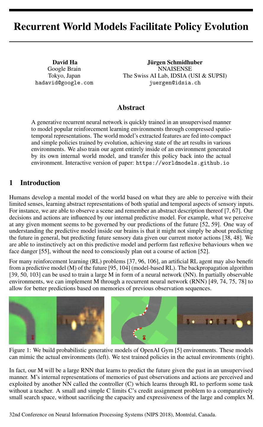
Training autonomous artificial intelligence systems directly within complex real-world or computationally heavy simulated environments is often expensive, slow, and resource intensive. The article investigates whether an agent can learn compact internal models of its environment and whether a decision-making policy trained entirely inside such an internally generated virtual world can successfully transfer back to the actual task.

The article demonstrates a modular architecture inspired by human cognition that separates visual perception, temporal prediction, and decision-making. High-dimensional visual observations are compressed into a compact spatial code using a vision model, while a recurrent memory model predicts future states and uncertainties based on past interactions. A very small, linear controller model with fewer than 1,100 parameters then determines actions based on these combined spatial and temporal representations. The controller is optimized using evolution strategies across simulated environments, including a continuous car racing benchmark and a survival simulation task.

The findings establish that the full predictive model solves the continuous car racing task from raw pixels, achieving a state-of-the-art score of 906, substantially outperforming existing deep reinforcement learning baselines that scored between 591 and 652. In contrast, an agent restricted to visual perception without temporal memory scored only 632. Furthermore, in the survival task, the agent was trained completely inside its own internally generated simulation and successfully transferred to the actual environment, achieving an average survival score of 1,092 steps against a passing threshold of 750 and exceeding the existing leaderboard record of 820. The evaluation also revealed that agents trained in deterministic simulations tend to exploit model inaccuracies; introducing controlled random uncertainty into the internal simulation prevented this gaming behavior and produced robust real-world policies.

These results indicate that decoupling complex world modeling from policy decision-making can significantly cut the computational cost of running heavy simulation engines. Instead of expending heavy resources on repeated real-world interactions, agents can train quickly in efficient, compressed latent spaces. Decision-makers should evaluate this architecture for continuous control and simulation-to-real workflows, particularly where real-world training is costly or risky. Future development must incorporate iterative data collection and curiosity-driven exploration, as the current unsupervised setup relies on initial datasets gathered by random policies and may struggle with highly complex, state-dependent environments.

Dalle Molle Institute for Artificial Intelligence Research Google NNAISENSE learning environments recurrent neural networks reinforcement learning world models policy evolution evolution strategies

arXiv: 1809.01999 hardmaru/WorldModelsExperiments

Paper: Tutorial on Variational Autoencoders, Carl Doersch (2016). This tutorial covers the theoretical formulation and reparameterization trick of Variational Autoencoders, which serve as the spatial perception component (the V model) used to compress observations in recurrent world models.
Paper: A Recurrent Latent Variable Model for Sequential Data, Junyoung Chung et al. (2015). This work introduces Variational Recurrent Neural Networks that combine recurrent models with latent variables for sequential data, establishing the architectural foundation for the MDN-RNN predictive dynamics model (the M model).
Paper: Unsupervised Learning of Video Representations using LSTMs, Nitish Srivastava et al. (2015). It provides key foundational methods for unsupervised predictive modeling of video frames using recurrent neural networks to capture spatio-temporal representations.
Paper: Self-improving reactive agents based on reinforcement learning, planning and teaching, Longxin Lin (1992). This classic paper introduces the foundational concept of training reactive policies within learned environmental transition models via relaxation planning.
Paper: Deep Recurrent Q-Learning for Partially Observable MDPs, Matthew Hausknecht et al. (2015). It demonstrates how recurrent neural memory layers can integrate visual observations over time to manage partially observable environments.

Paper: Learning Latent Dynamics for Planning from Pixels, Danijar Hafner et al. (2018). This work directly builds upon World Models by introducing the Recurrent State-Space Model (RSSM) to learn latent dynamics and plan directly from pixel inputs using online trajectory optimization.
Paper: Dream to Control: Learning Behaviors by Latent Imagination, Danijar Hafner et al. (2019). Dreamer generalizes policy training inside world models by using analytic gradient backpropagation through latent imagination rather than evolutionary search.
Paper: Mastering Atari with Discrete World Models, Danijar Hafner et al. (2021). DreamerV2 extends the latent imagination paradigm established by World Models and Dreamer to discrete categorical latents, mastering complex Atari benchmarks.
Paper: LeWorldModel: Stable End-to-End Joint-Embedding Predictive Architecture from Pixels, Lucas Maes et al. (2026). This work explores stable, reward-free joint-embedding predictive architectures (JEPAs) for predictive world modeling directly from raw visual inputs.
Paper: Next-Latent Prediction Transformers Learn Compact World Models, Jayden Teoh et al. (2025). This paper advances world modeling by equipping modern transformer architectures with next-latent prediction objectives to learn compact internal state dynamics.

Cover for Recurrent World Models Facilitate Policy Evolution

Abstract

A generative recurrent neural network is quickly trained in an unsupervised manner to model popular reinforcement learning environments through compressed spatio-temporal representations. The world model's extracted features are fed into compact and simple policies trained by evolution, achieving state of the art results in various environments. We also train our agent entirely inside of an environment generated by its own internal world model, and transfer this policy back into the actual environment. Interactive version of paper at this https URL

Topics

learning environments recurrent neural networks reinforcement learning feedforward neural networks unsupervised learning method evolutionary process

Keywords

world models policy evolution evolution strategies deep reinforcement learning recurrent neural networks policy network policy search generative models hierarchical planning intrinsic motivation

1 Introduction
2 Agent Model
3 Car Racing Experiment: World Model for Feature Extraction
3.1 Experiment Results
4 VizDoom Experiment: Learning Inside of a Generated Environment
4.1 Experiment Setup
4.2 Cheating the World Model
5 Related Work
6 Discussion
A Supplementary Materials
A.1 Comparing V, M, C Model Sizes
A.2 Variational Autoencoder
A.3 Mixture Density Network + Recurrent Neural Network
A.4 Controller
A.5 Evolution Strategies
A.6 DoomRNN
References

Knowls

Knowl 1 — Modular V-M-C Architecture for Reinforcement Learning
model/method
The World Model agent architecture divides reinforcement learning into three decoupled components:
1. Vision Model ( $V$ ): A Convolutional Variational Autoencoder (ConvVAE) that compresses high-dimensional visual observations $o_t$ (such as $64 \times 64 \times 3$ RGB pixel images) at each time step $t$ into a low-dimensional latent representation vector $z_t \in \mathbb{R}^{N_z}$ .
2. Memory Model ( $M$ ): A recurrent neural network combined with a Mixture Density Network (MDN-RNN), implemented using Long Short-Term Memory (LSTM) units. It acts as a predictive dynamics model that outputs the conditional probability distribution $P(z_{t+1} \mid a_t, z_t, h_t)$ of the next latent state $z_{t+1}$ given the current action $a_t$ , the current latent representation $z_t$ , and the hidden state $h_t$ of the LSTM.
3. Controller ( $C$ ): A compact decision-making policy that determines the action $a_t$ based on the combined representations of the current visual encoding $z_t$ and the recurrent temporal memory $h_t$ .
By delegating visual abstraction to $V$ and temporal predictive dynamics to $M$ , the credit assignment problem for the policy is confined to the low-dimensional parameter space of $C$ , allowing $C$ to be trained effectively using derivative-free evolutionary strategies while $V$ and $M$ are trained using standard gradient-based backpropagation.
Knowl 2 — Four-Stage Training Procedure for World Model Agents
algorithm
The agent is trained in four sequential, decoupled stages using an unsupervised dataset collected from the environment:
Input: Environment $\mathcal{E}$ with image observations, action dimension $N_a$ , latent dimension $N_z$
Output: Trained Vision model $V$ , Memory model $M$ , and Controller policy $C$
1. Data Collection:
   Collect 10,000 episode rollouts from $\mathcal{E}$ using a uniform random action policy
   Store recorded observation frames $o_t$ and actions $a_t$
2. Train Vision Model ( $V$ ):
   Train a Convolutional Variational Autoencoder (ConvVAE) on the collected frames
   Optimize reconstruction loss ( $L^2$ error) plus Kullback-Leibler (KL) divergence to map frames $o_t \mapsto z_t \in \mathbb{R}^{N_z}$
3. Train Memory Model ( $M$ ):
   Pre-compute latent vectors $z_t$ for all recorded frames using $V$
   Train an MDN-RNN via teacher forcing to predict $P(z_{t+1} \mid a_t, z_t, h_t)$ as a mixture of Gaussians (and binary termination probability $P(\text{done}_{t+1})$ where applicable)
4. Policy Evolution ( $C$ ):
   Evolve parameters $W_c, b_c$ of Controller $C$ using Covariance-Matrix Adaptation Evolution Strategy (CMA-ES) to maximize cumulative expected rollout rewards
This decoupled procedure avoids end-to-end backpropagation through time across raw image frames and enables training $M$ on long sequence rollouts (e.g., 1000 frames) on a single GPU.
Knowl 3 — MDN-RNN Predictive Latent Dynamics Model
model/method
The memory component $M$ models the transition dynamics of the environment in latent space. At each time step $t$ , the recurrent network (LSTM) updates its internal state and outputs the parameters of a Mixture Density Network (MDN) representing $P(z_{t+1} \mid a_t, z_t, h_t)$ .

The output distribution is modeled as a factored mixture of $K$ Gaussian components with diagonal covariance matrices:

$P(z_{t+1} \mid a_t, z_t, h_t) = \sum_{k=1}^{K} \pi_k(h_t) \, \mathcal{N}\left(z_{t+1} \;\middle|\; \mu_k(h_t), \sigma_k(h_t)^2 I\right)$

where $\pi_k(h_t)$ is the mixture weight of the $k$ -th Gaussian component (satisfying $\sum_{k=1}^K \pi_k = 1$ and $\pi_k \ge 0$ ), $\mu_k(h_t) \in \mathbb{R}^{N_z}$ is the mean vector, and $\sigma_k(h_t) \in \mathbb{R}^{N_z}$ is the vector of standard deviations, all parameterized as linear projections from the LSTM hidden state $h_t$ .

During autoregressive rollout sampling, a temperature hyperparameter $\tau > 0$ scales the standard deviation and mixture logits to adjust sampling randomness:

$\hat{\sigma}_k = \sigma_k \cdot \tau^{1/2}, \quad \hat{\pi}_k = \frac{\exp(\ell_k / \tau)}{\sum_{j=1}^K \exp(\ell_j / \tau)}$

where $\ell_k$ is the unnormalized logit for mixture component $k$ .
Knowl 4 — Linear Controller Model and Evolutionary Optimization
model/method
The controller $C$ is a minimal linear mapping from the concatenated spatial latent code $z_t$ and temporal hidden state $h_t$ to the continuous action vector $a_t$ :

$a_t = \tanh\left(W_c \begin{bmatrix} z_t \\ h_t \end{bmatrix} + b_c\right)$

where $W_c \in \mathbb{R}^{N_a \times (N_z + N_h)}$ is the weight matrix, $b_c \in \mathbb{R}^{N_a}$ is the bias vector, $N_z$ is the latent space dimension, $N_h$ is the recurrent hidden state dimension (or the concatenated hidden and cell states $[h_t, c_t]$ ), and $N_a$ is the action dimension. Bounding nonlinearities ( $anh$ or scaled shifts) clip each action dimension into its valid control range.

The parameter vector $\theta = \{W_c, b_c\}$ contains very few parameters (e.g., 867 parameters for CarRacing-v0 and 1,088 parameters for DoomTakeCover-v0). It is optimized using Covariance-Matrix Adaptation Evolution Strategy (CMA-ES) with a population size of 64. Fitness evaluation for each candidate solution is computed as the average cumulative reward across 16 independent environment rollouts with different initial random seeds.

Knowl 5 — CarRacing-v0 Continuous Control Benchmark Evaluation

data/table

The CarRacing-v0 benchmark requires an agent to steer, accelerate, and brake on top-down randomly generated race tracks directly from $64 \times 64 \times 3$ pixel inputs. A score of 900 or higher over 100 consecutive trials is defined as solving the environment.

Method	Average Score
DQN	$343 \pm 18$
A3C (continuous)	$591 \pm 45$
A3C (discrete)	$652 \pm 10$
Gym Leader	$838 \pm 11$
$V$ model only ( $a_t = W_c z_t + b_c$ )	$632 \pm 251$
$V$ model with hidden layer	$788 \pm 141$
Full World Model ( $V$ and $M$ )	$906 \pm 21$

The controller utilizing only the static latent representation $z_t$ from $V$ struggles on sharp corners due to lack of temporal context, achieving $632 \pm 251$ (or $788 \pm 141$ with an added hidden layer of 40 tanh units). Providing the controller access to both current latent state $z_t$ and recurrent hidden state $h_t$ enables instinctive predictive driving, attaining a score of $906 \pm 21$ over 100 random trials (and $900.46$ averaged over 1,024 trials), successfully solving the benchmark without task-specific image preprocessing.

Knowl 6 — Policy Training Entirely Inside a Hallucinated Latent Environment
model/method
Instead of interacting with a physical environment or simulator during reinforcement learning, the controller $C$ can be trained entirely inside a virtual environment simulated by the predictive model $M$ (termed DoomRNN for VizDoom).

The virtual environment operates as follows:
1. The simulation state consists exclusively of the latent vector $z_t$ and the recurrent hidden state $h_t$ , removing the requirement to render or encode $64 \times 64 \times 3$ pixel frames during rollout generation.
2. Given action $a_t$ from $C$ , the MDN-RNN transitions the hidden state to $h_{t+1}$ and samples $z_{t+1} \sim P(z_{t+1} \mid a_t, z_t, h_t)$ .
3. In addition to predicting $z_{t+1}$ , the MDN-RNN predicts the probability of episode termination $P(\text{done}_{t+1} \mid a_t, z_t, h_t)$ . The episode in the hallucinated environment terminates when this probability exceeds a fixed threshold of $0.5$ .
4. The environment is wrapped in a standard gym.Env interface. After evolutionary policy optimization completes entirely inside this virtual latent world, the trained controller is transferred directly to the actual environment without fine-tuning.
Knowl 7 — Temperature Regulation to Prevent Exploitation of Imperfect World Models
model/method
When an agent trains inside its own learned world model $M$ , it can discover adversarial policies that exploit model inaccuracies. In a deterministic or low-entropy simulation (such as sampling with temperature $\tau \le 0.1$ ), the learned dynamics model suffers from mode collapse: enemies fail to fire projectiles regardless of the agent's actions, or specific adversarial agent movement patterns cause projectiles to extinguish. The controller learns an exploit that achieves maximum survival scores (e.g., 2,100 steps) inside the hallucinated model but catastrophically fails when deployed in the actual environment.

To prevent exploitation:
1. $M$ is parameterized as a Mixture Density Network (MDN-RNN), modeling multi-modal probability distributions rather than deterministic point estimates.
2. The sampling temperature parameter $\tau$ is adjusted during generation. Setting $\tau > 1.0$ (e.g., $\tau = 1.15$ ) injects controlled stochasticity, forcing fireballs and state transitions to behave with higher uncertainty.
3. Training in a noisier and more uncertain virtual world prevents $C$ from relying on fragile, model-specific simulation exploits, yielding conservative and robust policies that transfer successfully to the real environment.

Knowl 8 — DoomTakeCover-v0 Virtual Training and Zero-Shot Transfer Performance

data/table

In DoomTakeCover-v0, an agent must dodge fireballs shot by monsters across a room to maximize survival time (maximum episode length is 2,100 steps; the task is considered solved if mean survival over 100 consecutive rollouts exceeds 750 steps). Controllers are trained entirely inside the virtual world model (DoomRNN) across varying temperature values $\tau$ and evaluated in both virtual and actual environments.

Temperature $\tau$	Virtual Score	Actual Score
0.10	$2086 \pm 140$	$193 \pm 58$
0.50	$2060 \pm 277$	$196 \pm 50$
1.00	$1145 \pm 690$	$868 \pm 511$
1.15	$918 \pm 546$	$1092 \pm 556$
1.30	$732 \pm 269$	$753 \pm 139$
Random Policy	N/A	$210 \pm 108$
Gym Leader	N/A	$820 \pm 58$

At low temperatures ( $\tau \le 0.50$ ), the controller exploits mode-collapsed hallucinations to score near the maximum ( $\approx 2086$ ), but fails completely in the real environment ( $\approx 193$ , worse than a random policy at $210 \pm 108$ ). At $\tau = 1.15$ , the virtual environment becomes harder than reality ( $918 \pm 546$ ), forcing the policy to learn robust dodging behaviors that achieve an average survival score of $1092 \pm 556$ in the actual game, solving the benchmark and outperforming the existing Gym Leader baseline ( $820 \pm 58$ ).

Knowl 9 — Architectural Specifications of V, M, and C Networks
model/method
The network dimensions and parameter counts for the CarRacing-v0 and DoomTakeCover-v0 tasks are structured as follows:
1. ConvVAE ( $V$ ):
  - Input: $64 \times 64 \times 3$ RGB image frames normalized to $[0, 1]$ .
  - Encoder: 4 convolutional layers with stride 2 and ReLU activations ( $32 \times \text{conv } 4\times 4$ , $64 \times \text{conv } 4\times 4$ , $128 \times \text{conv } 4\times 4$ , $256 \times \text{conv } 4\times 4$ ). Dense layers output mean $\mu$ and log-variance vectors of size $N_z$ .
  - Latent size $N_z$ : 32 for CarRacing-v0; 64 for DoomTakeCover-v0.
  - Decoder: Dense layer expanding $z$ to $1 \times 1 \times 1024$ , followed by 4 deconvolutional layers with stride 2 ( $128 \times \text{deconv } 5\times 5$ , $64 \times \text{deconv } 5\times 5$ , $32 \times \text{deconv } 6\times 6$ , and output $3 \times \text{deconv } 6\times 6$ with sigmoid activation).
  - Parameter count: 4,348,547 (CarRacing) / 4,446,915 (Doom).
2. MDN-RNN ( $M$ ):
  - Recurrent core: LSTM with 256 hidden units (CarRacing) / 512 hidden units (Doom).
  - MDN output: 5 Gaussian mixture components with factored diagonal covariance (no cross-correlation parameter $\rho$ ). Doom also includes a logistic output predicting termination $P(\text{done})$ .
  - Parameter count: 422,368 (CarRacing) / 1,678,785 (Doom).
3. Controller ( $C$ ):
  - CarRacing-v0: Linear model mapping $[z_t, h_t] \in \mathbb{R}^{32 + 256}$ to 3 continuous actions (steering, gas, brake), totaling 867 parameters.
  - DoomTakeCover-v0: Linear model mapping $[z_t, h_t, c_t] \in \mathbb{R}^{64 + 512 + 512}$ to 1 continuous action divided into 3 movement intervals (left, stay, right), totaling 1,088 parameters.
Knowl 10 — Limitations of Unsupervised Latent World Models
limitation
The decoupled V-M-C world model framework exhibits several key limitations:
1. Task-Agnostic Representation Loss: Because the ConvVAE ( $V$ ) is trained purely via pixel-level reconstruction and KL divergence without reward signals, it may prioritize encoding task-irrelevant visual patterns (such as detailed brick wall textures in Doom) while failing to encode small, task-critical features (such as distant track tiles or small obstacles).
2. Exploration Dependency on Random Rollouts: Training $V$ and $M$ on data collected from a uniform random exploration policy succeeds only in simple environments. In complex tasks where meaningful states can only be accessed through strategic navigation, the world model cannot learn dynamics for unvisited regions without an iterative exploration mechanism (e.g., curiosity-driven intrinsic motivation).
3. Limited Long-Term Memory Capacity: Fixed-size LSTM hidden states have finite memory capacity and are susceptible to catastrophic forgetting over long episodes.
4. Step-by-Step Simulation Without Hierarchical Planning: The MDN-RNN generates future states step-by-step at a low level of abstraction, lacking hierarchical planning or abstract multi-step reasoning capabilities.

Coverage note — No substantial contributed material was omitted. All primary model formulations, training algorithms, benchmark experimental results on CarRacing-v0 and DoomTakeCover-v0, temperature-exploitation analyses, and model architecture details are covered.

References

1.S. Alvernaz and J. Togelius. Autoencoder-augmented neuroevolution for visual doom playing. In Computational Intelligence and Games (CIG), 2017 IEEE Conference on, pages 1–8. IEEE, 2017.
2.T. M. Bartol Jr, C. Bromer, J. Kinney, M. A. Chirillo, J. N. Bourne, K. M. Harris, and T. J. Sejnowski. Nanoconnectomic upper bound on the variability of synaptic plasticity. Elife, 4, 2015.
3.C. M. Bishop. Neural networks for pattern recognition (chapter 6). Oxford university press, 1995.
4.K. Bousmalis, A. Irpan, P. Wohlhart, Y. Bai, M. Kelcey, M. Kalakrishnan, L. Downs, J. Ibarz, P. Pastor, K. Konolige, S. Levine, and V. Vanhoucke. Using simulation and domain adaptation to improve efficiency of deep robotic grasping. Preprint arXiv:1709.07857, Sept. 2017.
5.G. Brockman, V. Cheung, L. Pettersson, J. Schneider, J. Schulman, J. Tang, and W. Zaremba. OpenAI Gym. Preprint arXiv:1606.01540, June 2016.
6.S. Carter, D. Ha, I. Johnson, and C. Olah. Experiments in handwriting with a neural network. Distill, https://distill.pub/2016/handwriting, 2016.
7.L. Chang and D. Y. Tsao. The code for facial identity in the primate brain. Cell, 169(6):1013–1028, 2017.
8.S. Chiappa, S. Racaniere, D. Wierstra, and S. Mohamed. Recurrent environment simulators. Preprint arXiv:1704.02254, Apr. 2017.
9.M. Consalvo. Cheating: Gaining Advantage in Videogames (Chapter 5). The MIT Press, 2007.
10.M. Deisenroth and C. E. Rasmussen. PILCO: A model-based and data-efficient approach to policy search. In Proceedings of the 28th International Conference on machine learning (ICML-11), pages 465–472, 2011.
11.E. L. Denton et al. Unsupervised learning of disentangled representations from video. In Advances in Neural Information Processing Systems, pages 4417–4426, 2017.
12.S. Depeweg, J. M. Hernández-Lobato, F. Doshi-Velez, and S. Udluft. Learning and policy search in stochastic dynamical systems with bayesian neural networks. Preprint arXiv:1605.07127, May 2016.
13.A. Dosovitskiy and V. Koltun. Learning to act by predicting the future. Preprint arXiv:1611.01779, Nov. 2016.
14.C. Fernando, D. Banarse, C. Blundell, Y. Zwols, D. Ha, A. Rusu, A. Pritzel, and D. Wierstra. Pathnet: Evolution channels gradient descent in super neural networks. Preprint arXiv:1701.08734, Jan. 2017.
15.C. Finn, X. Y. Tan, Y. Duan, T. Darrell, S. Levine, and P. Abbeel. Deep spatial autoencoders for visuomotor learning. In Robotics and Automation (ICRA), 2016 IEEE International Conference on, pages 512–519. IEEE, 2016.
16.R. M. French. Catastrophic interference in connectionist networks: Can it be predicted, can it be prevented? In J. D. Cowan, G. Tesauro, and J. Alspector, editors, Advances in Neural Information Processing Systems 6, pages 1176–1177. Morgan-Kaufmann, 1994.
17.Y. Gal, R. McAllister, and C. E. Rasmussen. Improving PILCO with bayesian neural network dynamics models. In Data-Efficient Machine Learning workshop, ICML, 2016.
18.J. Gauci and K. O. Stanley. Autonomous evolution of topographic regularities in artificial neural networks. Neural Computation, 22(7):1860–1898, July 2010.
19.M. Gemici, C. Hung, A. Santoro, G. Wayne, S. Mohamed, D. Rezende, D. Amos, and T. Lillicrap. Generative temporal models with memory. Preprint arXiv:1702.04649, Feb. 2017.
20.F. Gers, J. Schmidhuber, and F. Cummins. Learning to forget: Continual prediction with LSTM. Neural Computation, 12(10):2451–2471, Oct. 2000.
21.F. Gomez and J. Schmidhuber. Co-evolving recurrent neurons learn deep memory POMDPs. Proceedings of the 7th Annual Conference on Genetic and Evolutionary Computation, pages 491–498, 2005.
22.F. Gomez, J. Schmidhuber, and R. Miikkulainen. Accelerated neural evolution through cooperatively coevolved synapses. Journal of Machine Learning Research, 9:937–965, June 2008.
23.J. Gottlieb, P.-Y. Oudeyer, M. Lopes, and A. Baranes. Information-seeking, curiosity, and attention: computational and neural mechanisms. Trends in cognitive sciences, 17(11):585–593, 2013.
24.A. Graves. Generating sequences with recurrent neural networks. Preprint arXiv:1308.0850, 2013.
25.A. Graves. Hallucination with recurrent neural networks. https://youtu.be/-yX1SYeDHbg, 2015.
26.D. Ha. Evolving stable strategies. http://blog.otoro.net/, 2017.
27.D. Ha, A. Dai, and Q. V. Le. Hypernetworks. In International Conference on Learning Representations, 2017.
28.D. Ha and D. Eck. A neural representation of sketch drawings. In International Conference on Learning Representations, 2018.
29.N. Hansen. The CMA evolution strategy: A tutorial. Preprint arXiv:1604.00772, 2016.
30.N. Hansen and A. Ostermeier. Completely derandomized self-adaptation in evolution strategies. Evolutionary Computation, 9(2):159–195, June 2001.
31.M. Hausknecht, J. Lehman, R. Miikkulainen, and P. Stone. A neuroevolution approach to general Atari game playing. IEEE Transactions on Computational Intelligence and AI in Games, 6(4):355–366, 2014.
32.D. Hein, S. Depeweg, M. Tokic, S. Udluft, A. Hentschel, T. Runkler, and V. Sterzing. A benchmark environment motivated by industrial control problems. Preprint arXiv:1709.09480, Sept. 2017.
33.I. Higgins, A. Pal, A. A. Rusu, L. Matthey, C. P. Burgess, A. Pritzel, M. Botvinick, C. Blundell, and A. Lerchner. DARLA: Improving zero-shot transfer in reinforcement learning. Preprint arXiv:1707.08475, 2017.
34.S. Hochreiter and J. Schmidhuber. Long short-term memory. Neural computation, 9(8):1735–1780, 1997.
35.J. Hünermann. Self-driving cars in the browser. http://janhuenermann.com/, 2017.
36.S. Jang, J. Min, and C. Lee. Reinforcement car racing with A3C. https://goo.gl/58SKBp, 2017.
37.L. P. Kaelbling, M. L. Littman, and A. W. Moore. Reinforcement learning: a survey. Journal of AI research, 4:237–285, 1996.
38.G. Keller, T. Bonhoeffer, and M. Hübener. Sensorimotor mismatch signals in primary visual cortex of the behaving mouse. Neuron, 74(5):809 – 815, 2012.
39.H. J. Kelley. Gradient theory of optimal flight paths. ARS Journal, 30(10):947–954, 1960.
40.M. Kempka, M. Wydmuch, G. Runc, J. Toczek, and W. Jaskowski. VizDoom: A Doom-based AI research platform for visual reinforcement learning. In IEEE Conference on Computational Intelligence and Games, pages 341–348, Santorini, Greece, Sep 2016. IEEE. The best paper award.
41.M. Khan and O. Elibol. Car racing using reinforcement learning. https://goo.gl/neSBSx, 2016.
42.D. Kingma and M. Welling. Auto-encoding variational bayes. Preprint arXiv:1312.6114, 2013.
43.J. Kirkpatrick, R. Pascanu, N. Rabinowitz, J. Veness, G. Desjardins, A. A. Rusu, K. Milan, J. Quan, T. Ramalho, A. Grabska-Barwinska, et al. Overcoming catastrophic forgetting in neural networks. Proceedings of the National Academy of Sciences, 114(13):3521–3526, 2017.
44.O. Klimov. CarRacing-v0. http://gym.openai.com/, 2016.
45.J. Koutnik, G. Cuccu, J. Schmidhuber, and F. Gomez. Evolving large-scale neural networks for vision-based reinforcement learning. Proceedings of the 15th Annual Conference on Genetic and Evolutionary Computation, pages 1061–1068, 2013.
46.B. Lau. Using Keras and deep deterministic policy gradient to play TORCS. https://yanpanlau.github.io/, 2016.
47.J. Lehman and K. Stanley. Abandoning objectives: Evolution through the search for novelty alone. Evolutionary Computation, 19(2):189–223, 2011.
48.M. Leinweber, D. R. Ward, J. M. Sobczak, A. Attinger, and G. B. Keller. A sensorimotor circuit in mouse cortex for visual flow predictions. Neuron, 95(6):1420 – 1432.e5, 2017.
49.L. Lin. Reinforcement Learning for Robots Using Neural Networks. PhD thesis, Carnegie Mellon University, Pittsburgh, January 1993.
50.S. Linnainmaa. The representation of the cumulative rounding error of an algorithm as a taylor expansion of the local rounding errors. Master’s thesis, Univ. Helsinki, 1970.
51.M. O. R. Matthew Guzdial, Boyang Li. Game engine learning from video. In Proceedings of the Twenty-Sixth International Joint Conference on Artificial Intelligence, IJCAI-17, pages 3707–3713, 2017.
52.G. W. Maus, J. Fischer, and D. Whitney. Motion-dependent representation of space in area MT+. Neuron, 78(3):554–562, 2013.
53.R. McAllister and C. E. Rasmussen. Data-efficient reinforcement learning in continuous state-action Gaussian-POMDPs. In Advances in Neural Information Processing Systems, pages 2037–2046, 2017.
54.V. Mnih, K. Kavukcuoglu, D. Silver, A. Graves, I. Antonoglou, D. Wierstra, and M. Riedmiller. Playing Atari with deep reinforcement learning. Preprint arXiv:1312.5602, Dec. 2013.
55.D. Mobbs, C. C. Hagan, T. Dalgleish, B. Silston, and C. Prévost. The ecology of human fear: survival optimization and the nervous system. Frontiers in neuroscience, 9:55, 2015.
56.P. W. Munro. A dual back-propagation scheme for scalar reinforcement learning. Proceedings of the Ninth Annual Conference of the Cognitive Science Society, Seattle, WA, pages 165–176, 1987.
57.A. Nagabandi, G. Kahn, R. Fearing, and S. Levine. Neural network dynamics for model-based deep reinforcement learning with model-free fine-tuning. Preprint arXiv:1708.02596, Aug. 2017.
58.N. Nguyen and B. Widrow. The truck backer-upper: An example of self learning in neural networks. In Proceedings of the International Joint Conference on Neural Networks, pages 357–363. IEEE Press, 1989.
59.N. Nortmann, S. Rekauzke, S. Onat, P. König, and D. Jancke. Primary visual cortex represents the difference between past and present. Cerebral Cortex, 25(6):1427–1440, 2015.
60.J. Oh, X. Guo, H. Lee, R. L. Lewis, and S. Singh. Action-conditional video prediction using deep networks in Atari games. In Advances in Neural Information Processing Systems, pages 2863–2871, 2015.
61.P.-Y. Oudeyer, F. Kaplan, and V. V. Hafner. Intrinsic motivation systems for autonomous mental development. IEEE transactions on evolutionary computation, 11(2):265–286, 2007.
62.P. Paquette. DoomTakeCover-v0. https://gym.openai.com/, 2016.
63.M. Parker and B. D. Bryant. Neurovisual control in the Quake II environment. IEEE Transactions on Computational Intelligence and AI in Games, 4(1):44–54, 2012.
64.D. Pathak, P. Agrawal, A. A. Efros, and T. Darrell. Curiosity-driven exploration by self-supervised prediction. In International Conference on Machine Learning (ICML), volume 2017, 2017.
65.H.-J. Pi, B. Hangya, D. Kvitsiani, J. I. Sanders, Z. J. Huang, and A. Kepecs. Cortical interneurons that specialize in disinhibitory control. Nature, 503(7477):521, 2013.
66.L. Prieur. Deep-Q Learning for racecar reinforcement learning problem. https://goo.gl/VpDqSw, 2017.
67.R. Q. Quiroga, L. Reddy, G. Kreiman, C. Koch, and I. Fried. Invariant visual representation by single neurons in the human brain. Nature, 435(7045):1102, 2005.
68.S. Racanière, T. Weber, D. Reichert, L. Buesing, A. Guez, D. J. Rezende, A. P. Badia, O. Vinyals, N. Heess, Y. Li, et al. Imagination-augmented agents for deep reinforcement learning. In Advances in Neural Information Processing Systems, pages 5694–5705, 2017.
69.R. M. Ratcliff. Connectionist models of recognition memory: constraints imposed by learning and forgetting functions. Psychological review, 97 2:285–308, 1990.
70.I. Rechenberg. Evolutionsstrategien. In Simulationsmethoden in der Medizin und Biologie, pages 83–114. Springer, 1978.
71.D. Rezende, S. Mohamed, and D. Wierstra. Stochastic backpropagation and approximate inference in deep generative models. Preprint arXiv:1401.4082, 2014.
72.T. Robinson and F. Fallside. Dynamic reinforcement driven error propagation networks with application to game playing. In Proceedings of the 11th Conference of the Cognitive Science Society, Ann Arbor, pages 836–843, 1989.
73.T. Salimans, J. Ho, X. Chen, S. Sidor, and I. Sutskever. Evolution strategies as a scalable alternative to reinforcement learning. Preprint arXiv:1703.03864, 2017.
74.J. Schmidhuber. Making the world differentiable: On using supervised learning fully recurrent neural networks for dynamic reinforcement learning and planning in non-stationary environments. Technische Universität München Tech. Report: FKI-126-90, 1990.
75.J. Schmidhuber. An on-line algorithm for dynamic reinforcement learning and planning in reactive environments. In Neural Networks, 1990., 1990 IJCNN International Joint Conference on, pages 253–258. IEEE, 1990.
76.J. Schmidhuber. A possibility for implementing curiosity and boredom in model-building neural controllers. Proceedings of the First International Conference on Simulation of Adaptive Behavior on From Animals to Animats, pages 222–227, 1990.
77.J. Schmidhuber. Curious model-building control systems. In Neural Networks, 1991. 1991 IEEE International Joint Conference on, pages 1458–1463. IEEE, 1991.
78.J. Schmidhuber. Reinforcement learning in markovian and non-markovian environments. In Advances in neural information processing systems, pages 500–506, 1991.
79.J. Schmidhuber. Learning complex, extended sequences using the principle of history compression. Neural Computation, 4(2):234–242, 1992. (Based on TR FKI-148-91, TUM, 1991).
80.J. Schmidhuber. Developmental robotics, optimal artificial curiosity, creativity, music, and the fine arts. Connection Science, 18(2):173–187, 2006.
81.J. Schmidhuber. Formal theory of creativity, fun, and intrinsic motivation (1990–2010). IEEE Transactions on Autonomous Mental Development, 2(3):230–247, 2010.
82.J. Schmidhuber. Powerplay: Training an increasingly general problem solver by continually searching for the simplest still unsolvable problem. Frontiers in Psychology, 4:313, 2013.
83.J. Schmidhuber. On learning to think: Algorithmic information theory for novel combinations of reinforcement learning controllers and recurrent neural world models. Preprint arXiv:1511.09249, 2015.
84.J. Schmidhuber. One big net for everything. Preprint arXiv:1802.08864, Feb. 2018.
85.J. Schmidhuber and R. Huber. Learning to generate artificial fovea trajectories for target detection. International Journal of Neural Systems, 2(1-2):125–134, 1991.
86.J. Schmidhuber, J. Storck, and S. Hochreiter. Reinforcement driven information acquisition in nondeterministic environments. Technical Report FKI- -94, TUM Department of Informatics, 1994.
87.H. Schwefel. Numerical Optimization of Computer Models. John Wiley and Sons, Inc., New York, NY, USA, 1977.
88.F. Sehnke, C. Osendorfer, T. Rückstieß, A. Graves, J. Peters, and J. Schmidhuber. Parameter-exploring policy gradients. Neural Networks, 23(4):551–559, 2010.
89.N. Shazeer, A. Mirhoseini, K. Maziarz, A. Davis, Q. Le, G. Hinton, and J. Dean. Outrageously large neural networks: The sparsely-gated mixture-of-experts layer. In International Conference on Learning Representations, 2017.
90.D. Silver, H. van Hasselt, M. Hessel, T. Schaul, A. Guez, T. Harley, G. Dulac-Arnold, D. Reichert, N. Rabinowitz, A. Barreto, and T. Degris. The predictron: End-to-end learning and planning. Preprint arXiv:1612.08810, Dec. 2016.
91.R. K. Srivastava, B. R. Steunebrink, and J. Schmidhuber. First experiments with powerplay. Neural Networks, 41:130–136, 2013.
92.K. O. Stanley and R. Miikkulainen. Evolving neural networks through augmenting topologies. Evolutionary computation, 10(2):99–127, 2002.
93.J. Suarez. Language modeling with recurrent highway hypernetworks. In I. Guyon, U. V. Luxburg, S. Bengio, H. Wallach, R. Fergus, S. Vishwanathan, and R. Garnett, editors, Advances in Neural Information Processing Systems 30, pages 3269–3278. Curran Associates, Inc., 2017.
94.F. P. Such, V. Madhavan, E. Conti, J. Lehman, K. O. Stanley, and J. Clune. Deep neuroevolution: Genetic algorithms are a competitive alternative for training deep neural networks for reinforcement learning. Preprint arXiv:1712.06567, Dec. 2017.
95.R. S. Sutton. Integrated architectures for learning, planning, and reacting based on approximating dynamic programming. In Machine Learning Proceedings 1990, pages 216–224. Elsevier, 1990.
96.R. S. Sutton and A. G. Barto. Introduction to Reinforcement Learning. MIT Press, Cambridge, MA, USA, 1st edition, 1998.
97.A. van den Oord, S. Dieleman, H. Zen, K. Simonyan, O. Vinyals, A. Graves, N. Kalchbrenner, A. Senior, and K. Kavukcuoglu. Wavenet: A generative model for raw audio. Preprint arXiv:1609.03499, Sept. 2016.
98.A. Vaswani, N. Shazeer, N. Parmar, J. Uszkoreit, L. Jones, A. N. Gomez, Ł. Kaiser, and I. Polosukhin. Attention is all you need. In Advances in Neural Information Processing Systems, pages 6000–6010, 2017.
99.N. Wahlström, T. B. Schön, and M. P. Desienroth. Learning deep dynamical models from image pixels. In 17th IFAC Symposium on System Identification (SYSID), October 19-21, Beijing, China, 2015.
100.N. Wahlström, T. Schön, and M. Deisenroth. From pixels to torques: Policy learning with deep dynamical models. Preprint arXiv:1502.02251, June 2015.
101.M. Watter, J. Springenberg, J. Boedecker, and M. Riedmiller. Embed to control: A locally linear latent dynamics model for control from raw images. In Advances in neural information processing systems, pages 2746–2754, 2015.
102.N. Watters, A. Tacchetti, T. Weber, R. Pascanu, P. Battaglia, and D. Zoran. Visual interaction networks. Preprint arXiv:1706.01433, June 2017.
103.P. J. Werbos. Applications of advances in nonlinear sensitivity analysis. In System modeling and optimization, pages 762–770. Springer, 1982.
104.P. J. Werbos. Learning how the world works: Specifications for predictive networks in robots and brains. In Proceedings of IEEE International Conference on Systems, Man and Cybernetics, N.Y., 1987.
105.P. J. Werbos. Neural networks for control and system identification. In Decision and Control, 1989., Proceedings of the 28th IEEE Conference on, pages 260–265. IEEE, 1989.
106.M. Wiering and M. van Otterlo. Reinforcement Learning. Springer, 2012.
107.Y. Wu, G. Wayne, A. Graves, and T. Lillicrap. The Kanerva machine: A generative distributed memory. In International Conference on Learning Representations, 2018.

Citation

MLA

Ha, D., and J. Schmidhuber. “Recurrent World Models Facilitate Policy Evolution”. arXiv, 2018, http://arxiv.org/abs/1809.01999v1.

APA

Ha, D., & Schmidhuber, J. (2018). Recurrent World Models Facilitate Policy Evolution. arXiv. http://arxiv.org/abs/1809.01999v1

Chicago

Ha, D., and J. Schmidhuber. 2018. “Recurrent World Models Facilitate Policy Evolution”. arXiv. http://arxiv.org/abs/1809.01999v1.

Harvard

Ha, D. and Schmidhuber, J. (2018) “Recurrent World Models Facilitate Policy Evolution”, arXiv [Preprint]. Available at: http://arxiv.org/abs/1809.01999v1.

Vancouver

1. Ha D, Schmidhuber J (2018) Recurrent World Models Facilitate Policy Evolution. arXiv

BibTeX

@article{ha2018recurrent,
  title = {Recurrent World Models Facilitate Policy Evolution},
  author = {Ha, David and Schmidhuber, Jürgen},
  year = {2018},
  journal = {arXiv},
  url = {http://arxiv.org/abs/1809.01999v1},
  eprint = {1809.01999}
}

Metadata:arXiv

Source Code

This paper has an official code repository available. Click below to access the source code.

View Repository

Access the Paper

This paper is available from its original source. Click below to access the PDF.

Open PDF

License: https://creativecommons.org/licenses/by/4.0/

Recurrent World Models Facilitate Policy Evolution

Abstract

Topics

Keywords

Table of Contents

Knowls

Knowl 1 — Modular V-M-C Architecture for Reinforcement Learning

Knowl 2 — Four-Stage Training Procedure for World Model Agents

Knowl 3 — MDN-RNN Predictive Latent Dynamics Model

Knowl 4 — Linear Controller Model and Evolutionary Optimization

Knowl 5 — CarRacing-v0 Continuous Control Benchmark Evaluation

Knowl 6 — Policy Training Entirely Inside a Hallucinated Latent Environment

Knowl 7 — Temperature Regulation to Prevent Exploitation of Imperfect World Models