
Binarized Neural Networks: Training Neural Networks with Weights and Activations Constrained to $+1$ or $-1$
Matthieu Courbariaux$^{*}$ $^{1}$
$^{1}$Université de Montréal
Itay Hubara$^{*}$ $^{2}$
$^{2}$Technion - Israel Institute of Technology
Daniel Soudry$^{3}$
$^{3}$Columbia University
Ran El-Yaniv$^{2}$
$^{2}$Technion - Israel Institute of Technology
Yoshua Bengio$^{1,4}$
$^{1}$Université de Montréal $^{4}$CIFAR Senior Fellow
$^{*}$Indicates equal contribution. Ordering determined by coin flip.
Abstract
We introduce a method to train Binarized Neural Networks (BNNs) - neural networks with binary weights and activations at run-time. At training-time the binary weights and activations are used for computing the parameters gradients. During the forward pass, BNNs drastically reduce memory size and accesses, and replace most arithmetic operations with bit-wise operations, which is expected to substantially improve power-efficiency. To validate the effectiveness of BNNs we conduct two sets of experiments on the Torch7 and Theano frameworks. On both, BNNs achieved nearly state-of-the-art results over the MNIST, CIFAR-10 and SVHN datasets. Last but not least, we wrote a binary matrix multiplication GPU kernel with which it is possible to run our MNIST BNN 7 times faster than with an unoptimized GPU kernel, without suffering any loss in classification accuracy. The code for training and running our BNNs is available on-line.
Executive Summary: Deep neural networks deliver state-of-the-art accuracy across computer vision and language tasks, but their substantial computational and power demands present major operational bottlenecks. Today, these models rely heavily on power-intensive graphics processors, limiting practical deployment on low-power, mobile, and embedded hardware. As operational energy and memory access costs increasingly limit hardware performance, discovering ways to drastically compress neural networks without sacrificing accuracy has become an urgent industry and engineering priority.
The article demonstrates a method to train Binarized Neural Networks, in which weights and activations are constrained to binary values of plus one or minus one during both training-time gradient calculations and run-time inference. It evaluates whether drastically reducing arithmetic precision to single-bit representations can maintain competitive predictive accuracy while reducing memory overhead and accelerating computation.
To establish credibility across distinct environments, the approach was tested across two widely used software frameworks on three standard image classification benchmarks: MNIST handwritten digits, CIFAR-10 object images, and Street View House Numbers. The training algorithm maintains full-precision weight accumulators to capture small gradient updates while applying a straight-through estimator to pass gradients through discontinuous thresholding steps. To eliminate power-hungry arithmetic operations, the authors also developed multiplier-free training variants for normalization and optimization using bit-shift logic, and implemented a dedicated binary matrix multiplication GPU kernel leveraging single-instruction-multiple-data registers.
The findings show that highly quantized networks perform remarkably well. First, binarized models achieved classification error rates close to unconstrained, 32-bit floating-point networks across all tested datasets (achieving test error rates of 0.96% to 1.40% on MNIST, 2.53% to 2.80% on SVHN, and 10.15% to 11.40% on CIFAR-10). Second, by replacing 32-bit values with single-bit variables, memory footprints and memory access volumes shrink by a factor of 32, which directly mitigates the most energy-intensive component of modern computing hardware. Third, standard multiply-accumulate arithmetic is replaced by bitwise logic gates, enabling dedicated hardware to substitute heavy floating-point multipliers with compact single-slice logic. Fourth, the custom binary matrix multiplication GPU kernel executed an MNIST network 7 times faster than a baseline kernel without any loss in accuracy, while accelerating raw matrix multiplication by 23 times over a baseline kernel and 3.4 times over standard cuBLAS routines. Finally, analyzing convolutional layers revealed that only 42% of 2D binary filters were unique, allowing dedicated architectures to reduce convolutional time complexity by roughly 60% by eliminating redundant operations.
These results provide a viable path to dramatically reduce infrastructure costs, power consumption, and hardware real estate for machine learning inference. The binarization process acts as a form of regularizing noise, explaining why accuracy remains competitive rather than degrading severely. For engineering teams and edge deployments, this approach shifts the computational burden from complex arithmetic units to power-efficient bitwise operations, unlocking high-performance deep learning on battery-constrained devices.
Decision-makers and engineering teams exploring edge AI or hardware-accelerated inference should evaluate binarization techniques and custom bitwise kernels for inference workloads. Hardware teams designing application-specific integrated circuits should leverage bitwise logic and filter-reuse architectures to maximize throughput. Before enterprise-wide adoption across all domains, research and development teams should conduct pilot evaluations to extend these methods to recurrent models and larger, complex datasets such as ImageNet.
Confidence in these findings is strong for standard image classification benchmarks on both Torch7 and Theano frameworks. However, readers should note current limitations: full-precision weights are still required in memory during the training phase to accumulate gradients, and the benchmarks evaluated in the article were restricted to small-scale image classification tasks. Ongoing research into binary gradient propagation and larger architectures will clarify performance at broader enterprise scale.
1. Binarized Neural Networks
Section Summary: Binarized neural networks constrain both weights and activations to values of +1 or −1 during training and inference. This is achieved through a deterministic sign function or a stochastic version based on a hard-sigmoid probability, with the deterministic approach used in most cases except for certain activations at training time. Although forward and backward passes rely on these binary values, real-valued gradients are still accumulated to enable stable stochastic gradient descent, while the binarization itself introduces a regularization effect similar to dropout.
In this section, we detail our binarization function, show how we use it to compute the parameters gradients, and how we backpropagate through it.
1.1 Deterministic vs Stochastic Binarization
When training a BNN, we constrain both the weights and the activations to either $+1$ or $-1$. Those two values are very advantageous from a hardware perspective, as we explain in Section 4. In order to transform the real-valued variables into those two values, we use two different binarization functions, as in ([25]). Our first binarization function is deterministic:
$ x^b = {Sign}(x) = \left{ \begin{array}{ll} +1 & \text{if }x \geq 0,\ -1 & \text{otherwise},\end{array} \right. $
where $x^b$ is the binarized variable (weight or activation) and $x$ the real-valued variable. It is very straightforward to implement and works quite well in practice. Our second binarization function is stochastic:
$ \begin{aligned} x^b = \left{ \begin{array}{ll} +1 & \text{with probability }p = \sigma(x),\ -1 & \text{with probability }1-p,\end{array} \right. \end{aligned} $
where $\sigma$ is the "hard sigmoid" function:
$ \sigma(x) = {clip}(\frac{x+1}{2},0,1) = \max(0,\min(1,\frac{x+1}{2})). $
The stochastic binarization is more appealing than the sign function, but harder to implement as it requires the hardware to generate random bits when quantizing. As a result, we mostly use the deterministic binarization function (i.e, the sign function), with the exception of activations at train-time in some of our experiments.
1.2 Gradient Computation and Accumulation
Although our BNN training method uses binary weights and activation to compute the parameters gradients, the real-valued gradients of the weights are accumulated in real-valued variables, as per Algorithm 1. Real-valued weights are likely required for Stochasic Gradient Descent (SGD) to work at all. SGD explores the space of parameters in small and noisy steps, and that noise is averaged out by the stochastic gradient contributions accumulated in each weight. Therefore, it is important to keep sufficient resolution for these accumulators, which at first glance suggests that high precision is absolutely required.
Moreover, adding noise to weights and activations when computing the parameters gradients provide a form of regularization that can help to generalize better, as previously shown with variational weight noise ([26]), Dropout ([27, 28]) and DropConnect ([29]). Our method of training BNNs can be seen as a variant of Dropout, in which instead of randomly setting half of the activations to zero when computing the parameters gradients, we binarize both the activations and the weights.
Require: a minibatch of inputs and targets $(a_0,a^*)$,
previous weights $W$, previous BatchNorm parameters $\theta$,
weights initialization coefficients from ([32]) $\gamma$,
and previous learning rate $\eta$.
Ensure: updated weights $W^{t+1}$, updated BatchNorm parameters $\theta^{t+1}$ and updated learning rate $\eta^{t+1}$.
// 1. Computing the parameters gradients:
// 1.1. Forward propagation:
for $k=1$ to $L$ do
  $W_k^b \leftarrow Binarize(W_k)$
  $s_k \leftarrow a_{k-1}^b W_k^b$
  $a_k \leftarrow BatchNorm(s_k, \theta_k)$
  if $k < L$ then
    $a_k^b \leftarrow Binarize(a_k)$
  end if
end for
// 1.2. Backward propagation:
// Please note that the gradients are not binary.
Compute $g_{a_L}=\frac{\partial C}{\partial a_L}$ knowing $a_L$ and $a^*$
for $k=L$ to $1$ do
  if $k < L$ then
    $g_{a_k} \leftarrow g_{a_k^b} \circ 1_{|a_k|\leq 1}$
  end if
  $(g_{s_k}, g_{\theta_k}) \leftarrow BackBatchNorm(g_{a_k}, s_k,\theta_k)$
  $g_{a_{k-1}^b} \leftarrow g_{s_k} W_k^{b}$
  $g_{W_k^b} \leftarrow g_{s_k}^{\top} a_{k-1}^b$
end for
// 2. Accumulating the parameters gradients:
for $k=1$ to $L$ do
  $\theta_k^{t+1} \leftarrow Update(\theta_k, \eta, g_{\theta_k})$
  $W_k^{t+1} \leftarrow Clip(Update(W_k, \gamma_k \eta, g_{W_k^b}),-1,1)$
  $\eta^{t+1} \leftarrow \lambda \eta$
end for
[h]
Require: Values of $x$ over a mini-batch: $B=\{x_{1\ldots m}\}$;
Parameters to be learned: $\gamma$, $\beta$
Ensure: $\{y_i = BN(x_i,{\gamma,\beta})\}$
$\mu_B \leftarrow \frac{1}m\sum_{i=1}^m x_i$ // mini-batch mean
$C(x_i) \leftarrow (x_i-\mu_B)$
// centered input
 $\sigma_B^2\! \leftarrow \!\! \frac{1}m\sum_{i=1}^m\! (C(x_i)\!\!\ll\gg\!\! AP2(C(x_i)))\!$ // apx variance
$\hat{x_i} \leftarrow C(x_i)\ll\gg AP2((\sqrt{\sigma_B^2+\epsilon})^{-1})$ // normalize
$y_i \leftarrow AP2(\gamma)\ll\gg\hat{x_i}$ // scale and shift
Note: Hardware implementation of AP2 is as simple as extracting the index of the most significant bit from the number's binary representation.
Require: Values of $x$ over a mini-batch: $B=\{x_{1\ldots m}\}$;
Parameters to be learned: $\gamma$, $\beta$
Ensure: $\{y_i = BN(x_i,{\gamma,\beta})\}$
$\mu_B \leftarrow \frac{1}m\sum_{i=1}^m x_i$ // mini-batch mean
$C(x_i) \leftarrow (x_i-\mu_B)$
// centered input
 $\sigma_B^2\! \leftarrow \!\! \frac{1}m\sum_{i=1}^m\! (C(x_i)\!\!\ll\gg\!\! AP2(C(x_i)))\!$ // apx variance
$\hat{x_i} \leftarrow C(x_i)\ll\gg AP2((\sqrt{\sigma_B^2+\epsilon})^{-1})$ // normalize
$y_i \leftarrow AP2(\gamma)\ll\gg\hat{x_i}$ // scale and shift
Require: Previous parameters $\theta_{t-1}$ and their gradient $g_t$, and learning rate $\alpha$.
Ensure: Updated parameters $\theta_t$
// Biased 1st and 2nd raw moment estimates:
$m_t \gets \beta_1 \cdot m_{t-1} + (1-\beta_1) \cdot g_t$
$v_t \gets \max (\beta_2 \cdot v_{t-1} , |g_t| )$
// Updated parameters:
$\theta_t \gets \theta_{t-1} - (\alpha \ll\gg (1-\beta_1)) \cdot \hat{m}\ll\gg v_t^{-1})$
Require: a vector of 8-bit inputs $a_0$,
the binary weights $W^b$, and the BatchNorm parameters $\theta$.
Ensure: the MLP output $a_L$.
// 1. First layer:
$a_1 \leftarrow 0$
for $n=1$ to $8$ do
  $a_1 \leftarrow a_1 + 2^{n-1} \times {XnorDotProduct(a_0^n,W^b_1)}$
end for
$a_1^b \leftarrow {Sign(BatchNorm}(a_1,\theta_1))$
// 2. Remaining hidden layers:
for $k=2$ to $L-1$ do
  $a_k \leftarrow XnorDotProduct(a_{k-1}^b,W^b_k)$
  $a_k^b \leftarrow {Sign(BatchNorm}(a_k,\theta_k))$
end for
// 3. Output layer:
$a_L \leftarrow XnorDotProduct(a_{L-1}^b,W^b_L)$
$a_L \leftarrow BatchNorm(a_L,\theta_L)$
1.3 Propagating Gradients Through Discretization
The derivative of the sign function is zero almost everywhere, making it apparently incompatible with backpropagation, since the exact gradient of the cost with respect to the quantities before the discretization (pre-activations or weights) would be zero. Note that this remains true even if stochastic quantization is used. [33] studied the question of estimating or propagating gradients through stochastic discrete neurons. They found in their experiments that the fastest training was obtained when using the "straight-through estimator," previously introduced in [34]'s lectures.
We follow a similar approach but use the version of the straight-through estimator that takes into account the saturation effect, and does use deterministic rather than stochastic sampling of the bit. Consider the sign function quantization
$ q = {Sign}(r), $
and assume that an estimator $g_q$ of the gradient $\frac{\partial C}{\partial q}$ has been obtained (with the straight-through estimator when needed). Then, our straight-through estimator of $\frac{\partial C}{\partial r}$ is simply
$ g_r = g_q 1_{|r|\leq 1}. $
Note that this preserves the gradient's information and cancels the gradient when $r$ is too large. Not cancelling the gradient when $r$ is too large significantly worsens the performance. The use of this straight-through estimator is illustrated in Algorithm 1. The derivative $1_{|r|\leq 1}$ can also be seen as propagating the gradient through hard tanh, which is the following piece-wise linear activation function:
$ {Htanh}(x) = {Clip}(x,-1,1) = \max(-1,\min(1,x)). $
For hidden units, we use the sign function non-linearity to obtain binary activations, and for weights we combine two ingredients:
- Constrain each real-valued weight between -1 and 1, by projecting $w^r$ to -1 or 1 when the weight update brings $w^r$ outside of $[-1,1]$, i.e., clipping the weights during training, as per Algorithm 1. The real-valued weights would otherwise grow very large without any impact on the binary weights.
- When using a weight $w^r$, quantize it using $w^b = {Sign}(w^r)$.
This is consistent with the gradient canceling when $|w^r|>1$, according to 4.
1.4 Shift based Batch Normalization
Batch Normalization (BN) ([30]), accelerates the training and also seems to reduces the overall impact of the weights' scale. The normalization noise may also help to regularize the model. However, at train-time, BN requires many multiplications (calculating the standard deviation and dividing by it), namely, dividing by the running variance (the weighted mean of the training set activation variance). Although the number of scaling calculations is the same as the number of neurons, in the case of ConvNets this number is quite large. For example, in the CIFAR-10 dataset (using our architecture), the first convolution layer, consisting of only $128\times3\times3$ filter masks, converts an image of size $3\times32\times32$ to size $3\times128\times28\times28$, which is two orders of magnitude larger than the number of weights. To achieve the results that BN would obtain, we use a shift-based batch normalization (SBN) technique. detailed in Algorithm 2. SBN approximates BN almost without multiplications. In the experiment we conducted we did not observe accuracy loss when using the shift based BN algorithm instead of the vanilla BN algorithm.
1.5 Shift based AdaMax
The ADAM learning rule ([31]) also seems to reduce the impact of the weight scale. Since ADAM requires many multiplications, we suggest using instead the shift-based AdaMax we detail in Algorithm 3. In the experiment we conducted we did not observe accuracy loss when using the shift-based AdaMax algorithm instead of the vanilla ADAM algorithm.
1.6 First Layer
In a BNN, only the binarized values of the weights and activations are used in all calculations. As the output of one layer is the input of the next, all the layers inputs are binary, with the exception of the first layer. However, we do not believe this to be a major issue. First, in computer vision, the input representation typically has much fewer channels (e.g, Red, Green and Blue) than internal representations (e.g, 512). As a result, the first layer of a ConvNet is often the smallest convolution layer, both in terms of parameters and computations ([2]).
Second, it is relatively easy to handle continuous-valued inputs as fixed point numbers, with $m$ bits of precision. For example, in the common case of $8$-bit fixed point inputs:
$ \begin{aligned} s & = x \cdot w^b \ s & = \sum_{n=1}^{8} {2^{n-1} (x^n \cdot w^b),} \end{aligned} $
where $x$ is a vector of 1024 8-bit inputs, $x_1^8$ is the most significant bit of the first input, $w^b$ is a vector of 1024 1-bit weights, and $s$ is the resulting weighted sum. This trick is used in Algorithm 4.
2. Benchmark Results
Section Summary: The section reports benchmark tests of binary neural networks on standard image classification tasks using MLPs for MNIST digits and convolutional networks for CIFAR-10 and SVHN images. Across two software frameworks with minor differences in how activations were binarized and how training was optimized, the networks reached near state-of-the-art accuracy on all three datasets while using far less computation than full-precision models. Results are shown in a summary table of error rates along with plots of training progress and examples of the learned binary filters.
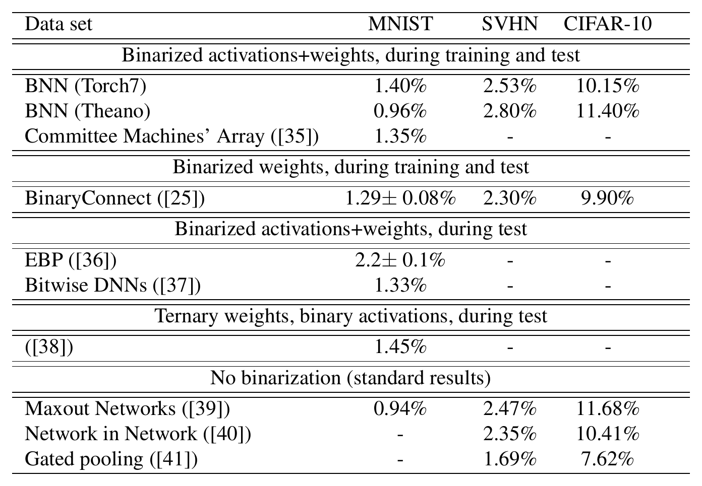
::: {caption="Table 1: Classification test error rates of DNNs trained on MNIST (MLP architecture without unsupervised pretraining), CIFAR-10 (without data augmentation) and SVHN."}
:::
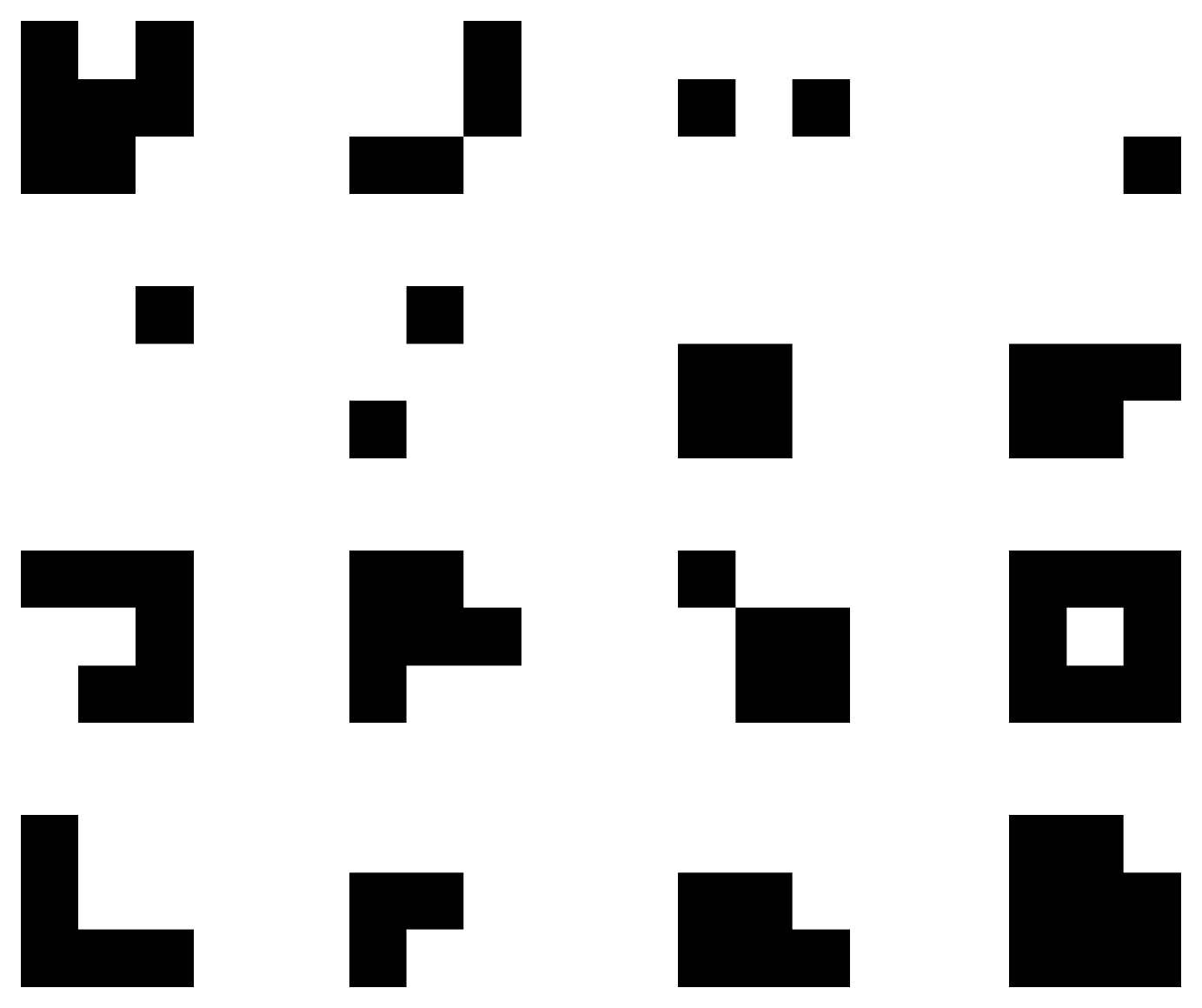
We conduct two sets of experiments, each based on a different framework, namely Torch7 ([22]) and Theano ([23, 24]). Other than the framework, the two sets of experiments are very similar:
- In both sets of experiments, we obtain near state-of-the-art results with BNNs on MNIST, CIFAR-10 and the SVHN benchmark datasets.
- In our Torch7 experiments, the activations are stochastically binarized at train-time, whereas in our Theano experiments they are deterministically binarized.
- In our Torch7 experiments, we use the shift-based BN and AdaMax variants, which are detailed in Algorithm 2 and Algorithm 3, whereas in our Theano experiments, we use vanilla BN and ADAM.
2.1 MLP on MNIST (Theano)
MNIST is an image classification benchmark dataset ([42]). It consists of a training set of 60K and a test set of 10K 28 $\times$ 28 gray-scale images representing digits ranging from 0 to 9. In order for this benchmark to remain a challenge, we did not use any convolution, data-augmentation, preprocessing or unsupervised learning. The MLP we train on MNIST consists of 3 hidden layers of 4096 binary units (see Section 1) and a L2-SVM output layer; L2-SVM has been shown to perform better than Softmax on several classification benchmarks ([43, 44]). We regularize the model with Dropout ([27, 28]). The square hinge loss is minimized with the ADAM adaptive learning rate method ([31]). We use an exponentially decaying global learning rate, as per Algorithm 1, and also scale the learning rates of the weights with their initialization coefficients from ([32]), as suggested by [25]. We use Batch Normalization with a minibatch of size 100 to speed up the training. As is typical, we use the last 10K samples of the training set as a validation set for early stopping and model selection. We report the test error rate associated with the best validation error rate after 1000 epochs (we do not retrain on the validation set). The results are reported in Table 1.
2.2 MLP on MNIST (Torch7)
We use a similar architecture as in our Theano experiments, without dropout, and with 2048 binary units per layer instead of 4096. Additionally, we use the shift base AdaMax and BN (with a minibatch of size 100) instead of the vanilla implementations, to reduce the number of multiplications. Likewise, we decay the learning rate by using a 1-bit right shift every 10 epochs. The results are presented in Table 1.
2.3 ConvNet on CIFAR-10 (Theano)
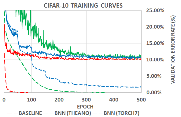
CIFAR-10 is an image classification benchmark dataset. It consists of a training set of size 50K and a test set of size 10K, where instance are 32 $\times$ 32 color images representing airplanes, automobiles, birds, cats, deer, dogs, frogs, horses, ships and trucks. We do not use any preprocessing or data-augmentation (which can really be a game changer for this dataset ([45])). The architecture of our ConvNet is the same architecture as [46]'s except for the binarization of the activations. [25]'s architecture is itself mainly inspired by VGG ([47]). The square hinge loss is minimized with ADAM. We use an exponentially decaying learning rate, as we did for MNIST. We scale the learning rates of the weights with their initialization coefficients from ([32]). We use Batch Normalization with a minibatch of size 50 to speed up the training. We use the last 5000 samples of the training set as a validation set. We report the test error rate associated with the best validation error rate after 500 training epochs (we do not retrain on the validation set). The results are presented in Table 1 and Figure 1.
2.4 ConvNet on CIFAR-10 (Torch7)
We use the same architecture as in our Theano experiments. We apply shift-based AdaMax and BN (with a minibatch of size 200) instead of the vanilla implementations to reduce the number of multiplications. Likewise, we decay the learning rate by using a 1-bit right shift every 50 epochs. The results are presented in Table 1 and Figure 1.
2.5 ConvNet on SVHN
SVHN is also an image classification benchmark dataset. It consists of a training set of size 604K examples and a test set of size 26K, where instances are 32 $\times$ 32 color images representing digits ranging from 0 to 9. In both sets of experiments, we follow the same procedure used for the CIFAR-10 experiments, with a few notable exceptions: we use half the number of units in the convolution layers, and we train for 200 epochs instead of 500 (because SVHN is a much larger dataset than CIFAR-10). The results are given in Table 1.
3. Very Power Efficient in Forward Pass
Section Summary: Binary neural networks slash energy use in the forward pass by shrinking memory size and accesses by a factor of 32 relative to ordinary 32-bit networks, an important saving because moving data to and from memory costs far more power than arithmetic itself. They also swap most floating-point multiplications for cheap single-bit XNOR and pop-count operations that need only minimal hardware. On top of this, binary weights produce many repeated two-dimensional filter patterns that can be reused, cutting the total number of operations by roughly 60 percent in practice.
: Table 2: Energy consumption of multiply-accumulations ([48])
| Operation | MUL | ADD |
|---|---|---|
| 8bit Integer | 0.2pJ | 0.03pJ |
| 32bit Integer | 3.1pJ | 0.1pJ |
| 16bit Floating Point | 1.1pJ | 0.4pJ |
| 32tbit Floating Point | 3.7pJ | 0.9pJ |
: Table 3: Energy consumption of memory accesses ([48])
| Memory size | 64-bit memory access |
|---|---|
| 8K | 10pJ |
| 32K | 20pJ |
| 1M | 100pJ |
| DRAM | 1.3-2.6nJ |
Computer hardware, be it general-purpose or specialized, is composed of memories, arithmetic operators and control logic. During the forward pass (both at run-time and train-time), BNNs drastically reduce memory size and accesses, and replace most arithmetic operations with bit-wise operations, which might lead to a great increase in power-efficiency. Moreover, a binarized CNN can lead to binary convolution kernel repetitions, and we argue that dedicated hardware could reduce the time complexity by $60%$ .
3.1 Memory Size and Accesses
Improving computing performance has always been and remains a challenge. Over the last decade, power has been the main constraint on performance ([48]). This is why much research effort has been devoted to reducing the energy consumption of neural networks. [48] provides rough numbers for the computations' energy consumption (the given numbers are for 45nm technology) as summarized in Table 2 and Table 3. Importantly, we can see that memory accesses typically consume more energy than arithmetic operations, and memory access' cost augments with memory size. In comparison with 32-bit DNNs, BNNs require 32 times smaller memory size and 32 times fewer memory accesses. This is expected to reduce energy consumption drastically (i.e., more than 32 times).
3.2 XNOR-Count
Applying a DNN mainly consists of convolutions and matrix multiplications. The key arithmetic operation of deep learning is thus the multiply-accumulate operation. Artificial neurons are basically multiply-accumulators computing weighted sums of their inputs. In BNNs, both the activations and the weights are constrained to either $-1$ or $+1$. As a result, most of the 32-bit floating point multiply-accumulations are replaced by 1-bit XNOR-count operations. This could have a big impact on deep learning dedicated hardware. For instance, a 32-bit floating point multiplier costs about 200 Xilinx FPGA slices ([49, 50]), whereas a 1-bit XNOR gate only costs a single slice.
3.3 Exploiting Filter Repetitions
When using a ConvNet architecture with binary weights, the number of unique filters is bounded by the filter size. For example, in our implementation we use filters of size $3\times3$, so the maximum number of unique 2D filters is $2^{9}=512$. However, this should not prevent expanding the number of feature maps beyond this number, since the actual filter is a 3D matrix. Assuming we have $M_{\ell}$ filters in the $\ell$ convolutional layer, we have to store a 4D weight matrix of size $M_{\ell}\times M_{\ell-1}\times k\times k$. Consequently, the number of unique filters is $2^{k^{2}M_{\ell-1}}$. When necessary, we apply each filter on the map and perform the required multiply-accumulate (MAC) operations (in our case, using XNOR and popcount operations). Since we now have binary filters, many 2D filters of size $k\times k$ repeat themselves. By using dedicated hardware/software, we can apply only the unique 2D filters on each feature map and sum the result wisely to receive each 3D filter's convolutional result. Note that an inverse filter (i.e., [-1,1, -1] is the inverse of [1, -1,1]) can also be treated as a repetition; it is merely a multiplication of the original filter by -1. For example, in our ConvNet architecture trained on the CIFAR-10 benchmark, there are only 42% unique filters per layer on average. Hence we can reduce the number of the XNOR-popcount operations by 3.
4. Seven Times Faster on GPU at Run-Time
Section Summary: By packing groups of 32 binary values into single registers, the SWAR technique lets GPUs perform many connections at once through simple bitwise operations such as XNOR and bit counting, yielding a theoretical speedup of roughly five times. In practice, a custom XNOR kernel built on this approach runs more than twenty times faster than a basic matrix-multiplication routine and over three times faster than the standard cuBLAS library when multiplying large binary matrices. When the same kernel is used inside the MNIST network, the full model finishes about seven times quicker than the unoptimized version while keeping identical accuracy.
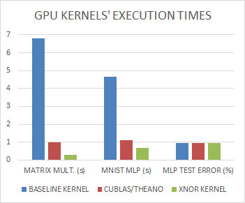
It is possible to speed up GPU implementations of BNNs, by using a method sometimes called SIMD (single instruction, multiple data) within a register (SWAR). The basic idea of SWAR is to concatenate groups of 32 binary variables into 32-bit registers, and thus obtain a 32-times speed-up on bitwise operations (e.g, XNOR). Using SWAR, it is possible to evaluate 32 connections with only 3 instructions:
$ a_1 += {popcount(xnor}(a_0^{32b},w^{32b}_1)), $
where $a_1$ is the resulting weighted sum, and $a_0^{32b}$ and $w^{32b}_1$ are the concatenated inputs and weights. Those 3 instructions (accumulation, popcount, xnor) take $1+4+1=6$ clock cycles on recent Nvidia GPUs (and if they were to become a fused instruction, it would only take a single clock cycle). Consequently, we obtain a theoretical Nvidia GPU speed-up of factor of $32/6 \approx 5.3$. In practice, this speed-up is quite easy to obtain as the memory bandwidth to computation ratio is also increased by 6 times.
In order to validate those theoretical results, we programed two GPU kernels:
- The first kernel (baseline) is a quite unoptimized matrix multiplication kernel.
- The second kernel (XNOR) is nearly identical to the baseline kernel, except that it uses the SWAR method, as in Equation (6).
The two GPU kernels return identical outputs when their inputs are constrained to $-1$ or $+1$ (but not otherwise). The XNOR kernel is about 23 times faster than the baseline kernel and 3.4 times faster than cuBLAS, as shown in Figure 3. Last but not least, the MLP from Section 2 runs 7 times faster with the XNOR kernel than with the baseline kernel, without suffering any loss in classification accuracy (see Figure 3).
5. Discussion and Related Work
Section Summary: Recent research overturned the view that binary neural networks must harm accuracy, showing instead that weights could be binarized throughout training or inference via methods such as Expectation BackPropagation and BinaryConnect, which treat quantization noise as a regularizer. Later efforts extended quantization to activations or back-propagation steps, yet still retained full-precision weights or limited binarization to only part of the computation. The present work is the first to binarize both weights and neurons for the entire training and inference of deep networks, yielding large efficiency gains while still requiring storage of real-valued weights during training.
Until recently, the use of extremely low-precision networks (binary in the extreme case) was believed to be highly destructive to the network performance ([51]). [52, 53] showed the contrary by showing that good performance could be achieved even if all neurons and weights are binarized to $\pm 1$ . This was done using Expectation BackPropagation (EBP), a variational Bayesian approach, which infers networks with binary weights and neurons by updating the posterior distributions over the weights. These distributions are updated by differentiating their parameters (e.g., mean values) via the back propagation (BP) algorithm. [21] implemented a fully binary network at run time using a very similar approach to EBP, showing significant improvement in energy efficiency. The drawback of EBP is that the binarized parameters were only used during inference.
The probabilistic idea behind EBP was extended in the BinaryConnect algorithm of [25]. In BinaryConnect, the real-valued version of the weights is saved and used as a key reference for the binarization process. The binarization noise is independent between different weights, either by construction (by using stochastic quantization) or by assumption (a common simplification; see Spang (1962). The noise would have little effect on the next neuron's input because the input is a summation over many weighted neurons. Thus, the real-valued version could be updated by the back propagated error by simply ignoring the binarization noise in the update. Using this method, [25] were the first to binarize weights in CNNs and achieved near state-of-the-art performance on several datasets. They also argued that noisy weights provide a form of regularization, which could help to improve generalization, as previously shown in ([29]). This method binarized weights while still maintaining full precision neurons.
[54] carried over the work of [25] to the back-propagation process by quantizing the representations at each layer of the network, to convert some of the remaining multiplications into binary shifts by restricting the neurons values of power-of-two integers. [54]'s work and ours seem to share similar characteristics . However, their approach continues to use full precision weights during the test phase. Moreover, [54] quantize the neurons only during the back propagation process, and not during forward propagation.
Other research [35] showed that fully binary training and testing is possible in an array of committee machines with randomized input, where only one weight layer is being adjusted. [55] and [56] aimed to compress a fully trained high precision network by using a quantization or matrix factorization methods. These methods required training the network with full precision weights and neurons, thus requiring numerous MAC operations avoided by the proposed BNN algorithm. [38] focused on a fixed-point neural network design and achieved performance almost identical to that of the floating-point architecture. [57] provided evidence that DNNs with ternary weights, used on a dedicated circuit, consume very low power and can be operated with only on-chip memory, at run time. [58] also indicated satisfactory empirical performance of neural networks with 8-bit precision. [59] retrained neural networks with binary weights and activations.
So far, to the best of our knowledge, no work has succeeded in binarizing weights and neurons, at the inference phase and the entire training phase of a deep network. This was achieved in the present work. We relied on the idea that binarization can be done stochastically, or be approximated as random noise. This was previously done for the weights by [25], but our BNNs extend this to the activations. Note that the binary activations are especially important for ConvNets, where there are typically many more neurons than free weights. This allows highly efficient operation of the binarized DNN at run time, and at the forward propagation phase during training. Moreover, our training method has almost no multiplications, and therefore might be implemented efficiently in dedicated hardware. However, we have to save the value of the full precision weights. This is a remaining computational bottleneck during training, since it requires relatively high energy resources. Novel memory devices might be used to alleviate this issue in the future; see e.g. [60].
Conclusion
Section Summary: Researchers have developed neural networks that use only binary values for their connections and internal calculations, both during operation and training. Experiments on standard image datasets show these networks achieve nearly top-level accuracy while using far less memory and replacing most math operations with simple bit-wise ones, leading to major gains in speed and energy efficiency. A custom graphics processor routine demonstrated a sevenfold speedup on one test case, with further work planned to extend these benefits to training and more complex models.
We have introduced BNNs, DNNs with binary weights and activations at run-time and when computing the parameters gradients at train-time (see Section 1). We have conducted two sets of experiments on two different frameworks, Torch7 and Theano, which show that it is possible to train BNNs on MNIST, CIFAR-10 and SVHN, and achieve nearly state-of-the-art results (see Section 2). Moreover, during the forward pass (both at run-time and train-time), BNNs drastically reduce memory size and accesses, and replace most arithmetic operations with bit-wise operations, which might lead to a great increase in power-efficiency (see Section 3). Last but not least, we programed a binary matrix multiplication GPU kernel with which it is possible to run our MNIST MLP 7 times faster than with an unoptimized GPU kernel, without suffering any loss in classification accuracy (see Section 4). Future works should explore how to extend the speed-up to train-time (e.g., by binarizing some gradients), and also extend benchmark results to other models (e.g, RNN) and datasets (e.g, ImageNet).
Acknowledgments
Section Summary: The authors thank Elad Hoffer for technical help and feedback, as well as their colleagues at the MILA lab for reviewing the work. They also credit the creators of software tools such as Torch, Theano, Pylearn2, and Lasagne, along with Yuxin Wu, for enabling fast and efficient code development on GPUs. Finally, they acknowledge financial support from CIFAR, NSERC, IBM, Samsung, and the Israel Science Foundation.
We would like to express our appreciation to Elad Hoffer, for his technical assistance and constructive comments. We thank our fellow MILA lab members who took the time to read the article and give us some feedback. We thank the developers of Torch, [22] a Lua based environment, and Theano ([23, 24]), a Python library which allowed us to easily develop a fast and optimized code for GPU. We also thank the developers of Pylearn2 ([61]) and Lasagne ([62]), two Deep Learning libraries built on the top of Theano. We thank Yuxin Wu for helping us compare our GPU kernels with cuBLAS. We are also grateful for funding from CIFAR, NSERC, IBM, Samsung, and the Israel Science Foundation (ISF).
References
Section Summary: This section compiles academic papers and technical reports primarily on deep neural networks and their applications in areas like image classification, speech recognition, machine translation, and game-playing AI systems. It also includes works on improving model efficiency through compression or hardware accelerators such as FPGAs and specialized chips, along with software tools and frameworks for training and deploying these models. The references span major conferences, journals, and workshops from roughly 2010 to 2016, highlighting rapid progress in scalable deep learning methods.
[1] Krizhevsky, A., Sutskever, I., and Hinton, G. ImageNet classification with deep convolutional neural networks. In NIPS'2012. 2012.
[2] Szegedy, Christian, Liu, Wei, Jia, Yangqing, Sermanet, Pierre, Reed, Scott, Anguelov, Dragomir, Erhan, Dumitru, Vanhoucke, Vincent, and Rabinovich, Andrew. Going deeper with convolutions. Technical report, arXiv:1409.4842, 2014.
[3] Hinton, Geoffrey, Deng, Li, Dahl, George E., Mohamed, Abdel-rahman, Jaitly, Navdeep, Senior, Andrew, Vanhoucke, Vincent, Nguyen, Patrick, Sainath, Tara, and Kingsbury, Brian. Deep neural networks for acoustic modeling in speech recognition. IEEE Signal Processing Magazine, 29(6):82–97, Nov. 2012.
[4] Sainath, Tara, rahman Mohamed, Abdel, Kingsbury, Brian, and Ramabhadran, Bhuvana. Deep convolutional neural networks for LVCSR. In ICASSP 2013, 2013.
[5] Devlin, Jacob, Zbib, Rabih, Huang, Zhongqiang, Lamar, Thomas, Schwartz, Richard, and Makhoul, John. Fast and robust neural network joint models for statistical machine translation. In Proc. ACL'2014, 2014.
[6] Sutskever, Ilya, Vinyals, Oriol, and Le, Quoc V. Sequence to sequence learning with neural networks. In NIPS'2014, 2014.
[7] Bahdanau, Dzmitry, Cho, Kyunghyun, and Bengio, Yoshua. Neural machine translation by jointly learning to align and translate. In ICLR'2015, arXiv:1409.0473, 2015.
[8] Mnih, Volodymyr, Kavukcuoglo, Koray, Silver, David, Rusu, Andrei A., Veness, Joel, Bellemare, Marc G., Graves, Alex, Riedmiller, Martin, Fidgeland, Andreas K., Ostrovski, Georg, Petersen, Stig, Beattie, Charles, Sadik, Amir, Antonoglou, Ioannis, King, Helen, Kumaran, Dharsan, Wierstra, Daan, Legg, Shane, and Hassabis, Demis. Human-level control through deep reinforcement learning. Nature, 518:529–533, 2015.
[9] Silver, David, Huang, Aja, Maddison, Chris J., Guez, Arthur, Sifre, Laurent, van den Driessche, George, Schrittwieser, Julian, Antonoglou, Ioannis, Panneershelvam, Veda, Lanctot, Marc, Dieleman, Sander, Grewe, Dominik, Nham, John, Kalchbrenner, Nal, Sutskever, Ilya, Lillicrap, Timothy, Leach, Madeleine, Kavukcuoglu, Koray, Graepel, Thore, and Hassabis, Demis. Mastering the game of go with deep neural networks and tree search. Nature, 529(7587):484–489, Jan 2016. Article.
[10] Mordvintsev, Alexander, Olah, Christopher, and Tyka, Mike. Inceptionism: Going deeper into neural networks, 2015. Accessed: 2015-06-30.
[11] Coates, Adam, Huval, Brody, Wang, Tao, Wu, David, Catanzaro, Bryan, and Andrew, Ng. Deep learning with COTS HPC systems. In Proceedings of the 30th international conference on machine learning, pp. 1337–1345, 2013.
[12] Vanhoucke, Vincent, Senior, Andrew, and Mao, Mark Z. Improving the speed of neural networks on CPUs. In Proc. Deep Learning and Unsupervised Feature Learning NIPS Workshop, 2011.
[13] Gong, Yunchao, Liu, Liu, Yang, Ming, and Bourdev, Lubomir. Compressing deep convolutional networks using vector quantization. arXiv preprint arXiv:1412.6115, 2014.
[14] Romero, Adriana, Ballas, Nicolas, Kahou, Samira Ebrahimi, Chassang, Antoine, Gatta, Carlo, and Bengio, Yoshua. Fitnets: Hints for thin deep nets. arXiv preprint arXiv:1412.6550, 2014.
[15] Han, Song, Pool, Jeff, Tran, John, and Dally, William. Learning both weights and connections for efficient neural network. In Advances in Neural Information Processing Systems, pp. 1135–1143, 2015.
[16] Farabet, Clément, LeCun, Yann, Kavukcuoglu, Koray, Culurciello, Eugenio, Martini, Berin, Akselrod, Polina, and Talay, Selcuk. Large-scale FPGA-based convolutional networks. Machine Learning on Very Large Data Sets, 1, 2011a.
[17] Farabet, Clément, Martini, Berin, Corda, Benoit, Akselrod, Polina, Culurciello, Eugenio, and LeCun, Yann. Neuflow: A runtime reconfigurable dataflow processor for vision. In Computer Vision and Pattern Recognition Workshops (CVPRW), 2011 IEEE Computer Society Conference on, pp. 109–116. IEEE, 2011b.
[18] Pham, Phi-Hung, Jelaca, Darko, Farabet, Clement, Martini, Berin, LeCun, Yann, and Culurciello, Eugenio. Neuflow: dataflow vision processing system-on-a-chip. In Circuits and Systems (MWSCAS), 2012 IEEE 55th International Midwest Symposium on, pp. 1044–1047. IEEE, 2012.
[19] Chen, Tianshi, Du, Zidong, Sun, Ninghui, Wang, Jia, Wu, Chengyong, Chen, Yunji, and Temam, Olivier. Diannao: A small-footprint high-throughput accelerator for ubiquitous machine-learning. In Proceedings of the 19th international conference on Architectural support for programming languages and operating systems, pp. 269–284. ACM, 2014a.
[20] Chen, Yunji, Luo, Tao, Liu, Shaoli, Zhang, Shijin, He, Liqiang, Wang, Jia, Li, Ling, Chen, Tianshi, Xu, Zhiwei, Sun, Ninghui, et al. Dadiannao: A machine-learning supercomputer. In Microarchitecture (MICRO), 2014 47th Annual IEEE/ACM International Symposium on, pp. 609–622. IEEE, 2014b.
[21] Esser, Steve K, Appuswamy, Rathinakumar, Merolla, Paul, Arthur, John V, and Modha, Dharmendra S. Backpropagation for energy-efficient neuromorphic computing. In Advances in Neural Information Processing Systems, pp. 1117–1125, 2015.
[22] Collobert, Ronan, Kavukcuoglu, Koray, and Farabet, Clément. Torch7: A matlab-like environment for machine learning. In BigLearn, NIPS Workshop, 2011.
[23] Bergstra, James, Breuleux, Olivier, Bastien, Frédéric, Lamblin, Pascal, Pascanu, Razvan, Desjardins, Guillaume, Turian, Joseph, Warde-Farley, David, and Bengio, Yoshua. Theano: a CPU and GPU math expression compiler. In Proceedings of the Python for Scientific Computing Conference (SciPy), June 2010. Oral Presentation.
[24] Bastien, Frédéric, Lamblin, Pascal, Pascanu, Razvan, Bergstra, James, Goodfellow, Ian J., Bergeron, Arnaud, Bouchard, Nicolas, and Bengio, Yoshua. Theano: new features and speed improvements. Deep Learning and Unsupervised Feature Learning NIPS 2012 Workshop, 2012.
[25] Courbariaux, Matthieu, Bengio, Yoshua, and David, Jean-Pierre. Binaryconnect: Training deep neural networks with binary weights during propagations. ArXiv e-prints, abs/1511.00363, November 2015.
[26] Graves, Alex. Practical variational inference for neural networks. In Advances in Neural Information Processing Systems, pp. 2348–2356, 2011.
[27] Srivastava, Nitish. Improving neural networks with dropout. Master's thesis, U. Toronto, 2013.
[28] Srivastava, Nitish, Hinton, Geoffrey, Krizhevsky, Alex, Sutskever, Ilya, and Salakhutdinov, Ruslan. Dropout: A simple way to prevent neural networks from overfitting. Journal of Machine Learning Research, 15:1929–1958, 2014.
[29] Wan, Li, Zeiler, Matthew, Zhang, Sixin, LeCun, Yann, and Fergus, Rob. Regularization of neural networks using dropconnect. In ICML'2013, 2013.
[30] Ioffe, Sergey and Szegedy, Christian. Batch normalization: Accelerating deep network training by reducing internal covariate shift. 2015.
[31] Kingma, Diederik and Ba, Jimmy. Adam: A method for stochastic optimization. arXiv preprint arXiv:1412.6980, 2014.
[32] Glorot, Xavier and Bengio, Yoshua. Understanding the difficulty of training deep feedforward neural networks. In AISTATS'2010, 2010.
[33] Bengio, Yoshua. Estimating or propagating gradients through stochastic neurons. Technical Report arXiv:1305.2982, Universite de Montreal, 2013.
[34] Hinton, Geoffrey. Neural networks for machine learning. Coursera, video lectures, 2012.
[35] Baldassi, Carlo, Ingrosso, Alessandro, Lucibello, Carlo, Saglietti, Luca, and Zecchina, Riccardo. Subdominant Dense Clusters Allow for Simple Learning and High Computational Performance in Neural Networks with Discrete Synapses. Physical Review Letters, 115(12):1–5, 2015.
[36] Cheng, Zhiyong, Soudry, Daniel, Mao, Zexi, and Lan, Zhenzhong. Training binary multilayer neural networks for image classification using expectation backpropgation. arXiv preprint arXiv:1503.03562, 2015.
[37] Kim, M. and Smaragdis, P. Bitwise Neural Networks. ArXiv e-prints, January 2016.
[38] Hwang, Kyuyeon and Sung, Wonyong. Fixed-point feedforward deep neural network design using weights+ 1, 0, and- 1. In Signal Processing Systems (SiPS), 2014 IEEE Workshop on, pp. 1–6. IEEE, 2014.
[39] Goodfellow, Ian J., Warde-Farley, David, Mirza, Mehdi, Courville, Aaron, and Bengio, Yoshua. Maxout Networks. arXiv preprint, pp. 1319–1327.
[40] Lin, Min, Chen, Qiang, and Yan, Shuicheng. Network In Network. arXiv preprint, pp. 10.
[41] Lee, Chen-Yu, Gallagher, Patrick W, and Tu, Zhuowen. Generalizing pooling functions in convolutional neural networks: Mixed, gated, and tree. arXiv preprint arXiv:1509.08985, 2015.
[42] LeCun, Yann, Bottou, Leon, Bengio, Yoshua, and Haffner, Patrick. Gradient-based learning applied to document recognition. Proceedings of the IEEE, 86(11):2278–2324, November 1998.
[43] Tang, Yichuan. Deep learning using linear support vector machines. Workshop on Challenges in Representation Learning, ICML, 2013.
[44] Lee, Chen-Yu, Xie, Saining, Gallagher, Patrick, Zhang, Zhengyou, and Tu, Zhuowen. Deeply-supervised nets. arXiv preprint arXiv:1409.5185, 2014.
[45] Graham, Benjamin. Spatially-sparse convolutional neural networks. arXiv preprint arXiv:1409.6070, 2014.
[46] Bibliography entry for citation key "Courbariaux2015" was not supplied with the source.
[47] Simonyan, Karen and Zisserman, Andrew. Very deep convolutional networks for large-scale image recognition. In ICLR, 2015.
[48] Horowitz, Mark. Computing's Energy Problem (and what we can do about it). IEEE Interational Solid State Circuits Conference, pp. 10–14, 2014.
[49] Govindu, Gokul, Zhuo, Ling, Choi, Seonil, and Prasanna, Viktor. Analysis of high-performance floating-point arithmetic on FPGAs. In Parallel and Distributed Processing Symposium, 2004. Proceedings. 18th International, pp. 149. IEEE, 2004.
[50] Beauchamp, Michael J, Hauck, Scott, Underwood, Keith D, and Hemmert, K Scott. Embedded floating-point units in FPGAs. In Proceedings of the 2006 ACM/SIGDA 14th international symposium on Field programmable gate arrays, pp. 12–20. ACM, 2006.
[51] Courbariaux, Matthieu, Bengio, Yoshua, and David, Jean-Pierre. Training deep neural networks with low precision multiplications. ArXiv e-prints, abs/1412.7024, December 2014.
[52] Soudry, Daniel, Hubara, Itay, and Meir, Ron. Expectation backpropagation: Parameter-free training of multilayer neural networks with continuous or discrete weights. In NIPS'2014, 2014.
[53] Bibliography entry for citation key "Cheng2015" was not supplied with the source.
[54] Lin, Zhouhan, Courbariaux, Matthieu, Memisevic, Roland, and Bengio, Yoshua. Neural networks with few multiplications. ArXiv e-prints, abs/1510.03009, October 2015.
[55] Judd, Patrick, Albericio, Jorge, Hetherington, Tayler, Aamodt, Tor, Jerger, Natalie Enright, Urtasun, Raquel, and Moshovos, Andreas. Reduced-Precision Strategies for Bounded Memory in Deep Neural Nets. pp. 12.
[56] Gong, Yunchao, Liu, Liu, Yang, Ming, and Bourdev, Lubomir. Compressing Deep Convolutional Networks using Vector Quantization. pp. 1–10.
[57] Kim, Jonghong, Hwang, Kyuyeon, and Sung, Wonyong. X1000 real-time phoneme recognition vlsi using feed-forward deep neural networks. In Acoustics, Speech and Signal Processing (ICASSP), 2014 IEEE International Conference on, pp. 7510–7514. IEEE, 2014.
[58] Sung, Wonyong, Shin, Sungho, and Hwang, Kyuyeon. Resiliency of Deep Neural Networks under Quantization. (2014):1–9.
[59] Kim, Minje and Paris, Smaragdis. Bitwise Neural Networks. ICML Workshop on Resource-Efficient Machine Learning, 37, 2015.
[60] Soudry, Daniel, Di Castro, Dotan, Gal, Asaf, Kolodny, Avinoam, and Kvatinsky, Shahar. Memristor-Based Multilayer Neural Networks With Online Gradient Descent Training. IEEE Transactions on Neural Networks and Learning Systems, (10):2408–2421.
[61] Goodfellow, Ian J., Warde-Farley, David, Lamblin, Pascal, Dumoulin, Vincent, Mirza, Mehdi, Pascanu, Razvan, Bergstra, James, Bastien, Frédéric, and Bengio, Yoshua. Pylearn2: a machine learning research library. arXiv preprint arXiv:1308.4214, 2013.
[62] Dieleman, Sander, Schlüter, Jan, Raffel, Colin, Olson, Eben, Sønderby, Søren Kaae, Nouri, Daniel, Maturana, Daniel, Thoma, Martin, Battenberg, Eric, Kelly, Jack, Fauw, Jeffrey De, Heilman, Michael, diogo149, McFee, Brian, Weideman, Hendrik, takacsg84, peterderivaz, Jon, instagibbs, Rasul, Dr. Kashif, CongLiu, Britefury, and Degrave, Jonas. Lasagne: First release., August 2015.