LSTM Fully Convolutional Networks for Time Series Classification

Fazle KarimSomshubra MajumdarHoushang DarabiShun Chen

article2017IEEE Access1,328 citations

Introduces LSTM-augmented fully convolutional neural networks that achieve state-of-the-art time series classification performance with minimal data preprocessing while enabling model decision visualization through attention mechanisms.

Listen

Time series classification is vital across multiple sectors, including finance, industrial monitoring, and healthcare. Traditional classification approaches and complex ensemble models require extensive manual feature engineering, heavy data preprocessing, and significant computational overhead. While modern deep learning architectures like fully convolutional networks have shown promise in automating this process, they often fail to capture long-term temporal sequence relationships effectively.

The article evaluates whether combining fully convolutional networks with recurrent sub-modules—specifically long short-term memory networks and attention-augmented versions—can improve time series classification accuracy while keeping model size and preprocessing requirements minimal.

The authors tested their proposed architectures, the Long Short-Term Memory Fully Convolutional Network and the Attention Long Short-Term Memory Fully Convolutional Network, across all 85 standard University of California Riverside time series benchmark datasets. The design feeds data concurrently into a three-layer temporal convolutional feature extractor and a recurrent branch. A crucial dimension-shuffle step transposes the sequence so the recurrent branch processes the series without severe overfitting or failing on long horizons. The evaluation also implemented an iterative fine-tuning process using decaying learning rates and halved batch sizes.

The experimental findings show that the proposed architectures significantly outperform previous state-of-the-art models across standard rank and error metrics. The fine-tuned basic recurrent hybrid achieved the highest overall success, outperforming previous benchmarks on 65 of the 85 datasets and reducing the mean per-class error. Statistical hypothesis testing confirmed these improvements are significant (p-values below 0.05). Additionally, the attention mechanism provided a clear visual decision trail by highlighting exact points in the time sequence that determine classification, although it added parameter complexity.

These results demonstrate that organizations can deploy high-performing time series classification models end-to-end without investing substantial resources into manual feature extraction or intricate preprocessing pipelines. For production environments where model interpretability and auditability are required, the attention-based architecture offers a clear view into decision pathways. When maximizing classification performance is the primary goal, the standard recurrent hybrid combined with fine-tuning delivers the best overall accuracy.

Next steps should focus on extending these architectures from single-variable time series to multivariate industrial datasets and investigating why the simpler recurrent sub-module occasionally outperforms the attention-augmented version. While the broad benchmark results provide high confidence in the models' general utility, practitioners should note that fine-tuning requires longer training runtimes due to iterative re-training with smaller batch sizes.

  • Paper: Time series classification from scratch with deep neural networks: A strong baseline, Zhiguang Wang et al. (2016). This paper establishes Fully Convolutional Networks (FCNs) as a baseline for end-to-end time series classification, which the source directly builds upon and augments with LSTM modules.
  • Paper: Long Short-Term Memory, Sepp Hochreiter et al. (1997). This foundational paper introduces the Long Short-Term Memory recurrent architecture that provides the core temporal sub-module integrated into the source paper's hybrid model.
  • Paper: Recurrent Convolutional Neural Networks for Text Classification, Siwei Lai et al. (2015). This work explores combining recurrent and convolutional neural network layers for sequence classification, serving as an architectural conceptual precursor to hybrid sequence modeling.
  • Paper: Understanding LSTM Networks, Christopher Olah (2015). This paper provides a detailed exposition of LSTM gating mechanics and state flow necessary to understand how recurrent sub-modules capture temporal dependencies alongside convolutional features.
Cover for LSTM Fully Convolutional Networks for Time Series Classification

Abstract

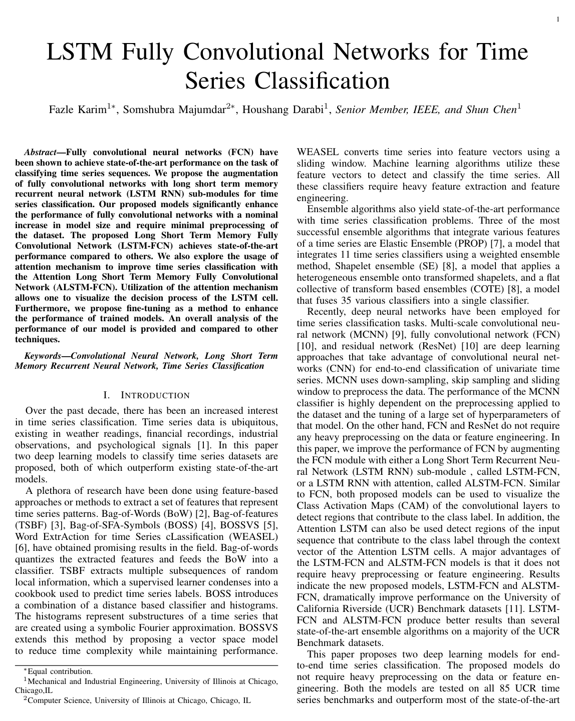
Fully convolutional neural networks (FCN) have been shown to achieve state-of-the-art performance on the task of classifying time series sequences. We propose the augmentation of fully convolutional networks with long short term memory recurrent neural network (LSTM RNN) sub-modules for time series classification. Our proposed models significantly enhance the performance of fully convolutional networks with a nominal increase in model size and require minimal preprocessing of the dataset. The proposed Long Short Term Memory Fully Convolutional Network (LSTM-FCN) achieves state-of-the-art performance compared to others. We also explore the usage of attention mechanism to improve time series classification with the Attention Long Short Term Memory Fully Convolutional Network (ALSTM-FCN). Utilization of the attention mechanism allows one to visualize the decision process of the LSTM cell. Furthermore, we propose fine-tuning as a method to enhance the performance of trained models. An overall analysis of the performance of our model is provided and compared to other techniques.

Table of Contents

  • I Introduction
  • II Background Works
  • II-A Temporal Convolutions
  • II-B Recurrent Neural Networks
  • II-C Long Short-Term Memory RNNs
  • II-D Attention Mechanism
  • III LSTM Fully Convolutional Network
  • III-A Network Architecture
  • III-B Network Input
  • III-C Fine-Tuning of Models
  • IV Experiments
  • IV-A Evaluation Metrics
  • IV-B Results
  • V Conclusion & Future Work
  • References

Knowls

  1. Knowl 1 — LSTM-FCN and ALSTM-FCN Network Architectures

    model/method

    The Long Short Term Memory Fully Convolutional Network (LSTM-FCN) and Attention LSTM Fully Convolutional Network (ALSTM-FCN) are dual-stream deep neural network architectures for end-to-end univariate time series classification.

    Given an input time series of length NN, the architecture processes the data concurrently through two parallel branches:

    1. Fully Convolutional Network (FCN) Branch: Views the input as a univariate sequence with NN time steps and 1 feature channel. It consists of three stacked 1D convolutional blocks followed by global average pooling:

      • Convolution Block 1: 1D temporal convolution with 128 filters, Batch Normalization (momentum 0.990.99, ϵ=0.001\epsilon = 0.001), and a Rectified Linear Unit (ReLU) activation.
      • Convolution Block 2: 1D temporal convolution with 256 filters, Batch Normalization (momentum 0.990.99, ϵ=0.001\epsilon = 0.001), and a ReLU activation.
      • Convolution Block 3: 1D temporal convolution with 128 filters, Batch Normalization (momentum 0.990.99, ϵ=0.001\epsilon = 0.001), and a ReLU activation.
      • Global Average Pooling (GAP) reduces the feature maps of the third block into a 128-dimensional representation.
    2. Recurrent (LSTM / Attention LSTM) Branch: Processes the input after passing it through a dimension shuffle layer that transposes the temporal axis into feature dimensions, presenting the input as a single time step with NN variables. This input is processed by:

      • A standard Long Short Term Memory (LSTM) layer in LSTM-FCN, or an Attention LSTM layer in ALSTM-FCN, containing between 8 and 128 hidden cells.
      • A dropout layer with a dropout rate of 0.80.8 (80%80\%) to mitigate overfitting.
    3. Classification Head: The 128-dimensional output from the global average pooling layer and the output vector from the LSTM/ALSTM dropout layer are concatenated into a single feature vector and passed into a final Softmax classification layer parameterized over CC target classes.

  2. Knowl 2 — Dimension Shuffle Layer for Recurrent Time Series Ingestion

    model/method

    The dimension shuffle layer transforms the temporal representation of an input time series specifically for the recurrent branch of LSTM-FCN and ALSTM-FCN.

    While the convolutional branch ingests a univariate time series of temporal length NN in standard sequence format (a univariate sequence across NN discrete time steps), the recurrent branch requires a transposed view. The dimension shuffle transposes the sequence so that the input is perceived by the LSTM or Attention LSTM block as a multivariate time series consisting of a single time step with NN feature variables.

    This structural transformation prevents the severe overfitting typically observed when standard LSTMs process short-sequence datasets, and avoids the vanishing gradient and memory degradation issues encountered when unrolling recurrent cells over long-sequence time series datasets.

  3. Knowl 3 — Iterative Same-Dataset Fine-Tuning Algorithm

    algorithm

    The fine-tuning algorithm enhances the classification performance of a pre-trained time series model by performing iterative transfer learning on the same training dataset across KK successive iterations (typically set to K=5K = 5).

    At each iteration, model weights are initialized from the checkpoint saved at the end of the previous iteration. The initial learning rate is halved at every iteration, and the batch size is halved every alternate iteration, continuing until reaching an initial learning rate of 10−410^{-4} and a batch size of 32.

    Input: Model MM with initial trained weights W0W_0, iteration count KK, initial learning rate α0\alpha_0, initial batch size B0B_0
    Output: Fine-tuned model MM
    W←W0W \leftarrow W_0
    α←α0\alpha \leftarrow \alpha_0
    B←B0B \leftarrow B_0
    for i=1i = 1 to KK do
        M←LoadWeights(M,W)M \leftarrow \text{LoadWeights}(M, W)
        M←Train(M,α,B)M \leftarrow \text{Train}(M, \alpha, B)
        W←GetWeights(M)W \leftarrow \text{GetWeights}(M)
        α←α/2\alpha \leftarrow \alpha / 2
        if i mod 2=0i \bmod 2 = 0 then
            B←max⁡(32,B/2)B \leftarrow \max(32, B / 2)
        end if
    end for
    return MM
  4. Knowl 4 — Attention LSTM Sub-module and Context Vector Visualization

    model/method

    In the ALSTM-FCN model, the recurrent stream employs an Attention Long Short-Term Memory cell based on the Bahdanau additive attention mechanism.

    For a sequence of hidden annotation vectors (h1,h2,…,hTx)(h_1, h_2, \dots, h_{T_x}) produced across the input, the attention context vector cic_i for output step ii is calculated as:

    ci=∑j=1Txαijhjc_i = \sum_{j=1}^{T_x} \alpha_{ij} h_j

    where the alignment weight αij\alpha_{ij} is computed via a softmax normalization over alignment energy scores eije_{ij}:

    αij=exp⁡(eij)∑k=1Txexp⁡(eik)\alpha_{ij} = \frac{\exp(e_{ij})}{\sum_{k=1}^{T_x} \exp(e_{ik})}

    Here, eij=a(si−1,hj)e_{ij} = a(s_{i-1}, h_j) is scored by a feedforward alignment neural network a(⋅)a(\cdot) conditioned on the previous recurrent hidden state si−1s_{i-1} and the annotation hjh_j.

    In addition to learning long-range dependencies, plotting the Attention LSTM context vectors provides visual interpretability for the network's classification decisions. Points in the temporal profile where the context vector sequences of distinct classes squeeze together designate time steps where class weights are identical and where the recurrent cell differentiates the classes based on distinct underlying temporal patterns.

  5. Knowl 5 — Mean Per-Class Error (MPCE) Metric

    definition

    Mean Per-Class Error (MPCE) is an aggregate evaluation metric used to benchmark time series classification models across heterogeneous datasets containing varying numbers of target classes.

    For a single dataset kk with classification accuracy accuracyk\text{accuracy}_k and CkC_k unique classes, the Per-Class Error PCEk\text{PCE}_k is defined as:

    PCEk=1−accuracykCk\text{PCE}_k = \frac{1 - \text{accuracy}_k}{C_k}

    For a benchmark collection comprising KK distinct datasets, the Mean Per-Class Error (MPCE) is the arithmetic mean of all individual per-class errors:

    MPCE=1K∑k=1KPCEk\text{MPCE} = \frac{1}{K} \sum_{k=1}^K \text{PCE}_k

    By scaling the classification error inversely by the number of classes CkC_k, MPCE prevents multi-class datasets with high class counts from dominating the aggregate benchmark error relative to datasets with fewer classes.

  6. Knowl 6 — Training Configuration and Hyperparameters on the UCR Benchmark Archive

    experimental setup

    Evaluation of LSTM-FCN and ALSTM-FCN is conducted across all 85 datasets in the University of California Riverside (UCR) Time Series Classification Archive without additional domain-specific feature engineering or preprocessing (exploiting zero mean and unit variance standard properties).

    • Weight Initialization: All 1D convolutional filter weights are initialized using He normal initialization.
    • Optimizer and Learning Rate Schedule: Trained using the Adam optimizer with an initial learning rate of 10−310^{-3} and a minimum lower bound of 10−410^{-4}. If the validation score fails to improve for 100 consecutive epochs, the learning rate is reduced by a factor of 1/23≈0.79371/\sqrt[3]{2} \approx 0.7937.
    • Epoch Budget and Batch Size: Base training lasts for 2000 epochs (extended on datasets with slow convergence) with an initial mini-batch size of 128.
    • Regularization and Search: A dropout rate of 0.80.8 is applied to the recurrent module. The number of LSTM / Attention LSTM units is tuned via hyperparameter search over {8,16,32,64,128}\{8, 16, 32, 64, 128\} cells.
    • Class Imbalance: Mitigated using an inverse-frequency class-weighting loss formulation.
  7. Knowl 7 — Classification Performance Across 85 UCR Benchmark Datasets

    empirical result

    Across all 85 datasets of the UCR Time Series Archive, both LSTM-FCN and ALSTM-FCN (evaluated with and without fine-tuning) consistently match or outperform prior state-of-the-art (SOTA) classifiers (including WEASEL, FCN, ResNet, COTE, and BOSS):

    • Number of Datasets Matching or Beating Prior SOTA (out of 85):

      • Base LSTM-FCN (Phase 1, no fine-tuning): 43 datasets
      • Fine-Tuned LSTM-FCN (Phase 2): 65 datasets
      • Base ALSTM-FCN (Phase 1, no fine-tuning): 51 datasets
      • Fine-Tuned ALSTM-FCN (Phase 2): 57 datasets
    • Mean Per-Class Error (MPCE):

      • Base LSTM-FCN: 0.03180.0318
      • Fine-Tuned LSTM-FCN: 0.02830.0283 (absolute MPCE reduction of 0.00350.0035)
      • Base ALSTM-FCN: 0.03010.0301
      • Fine-Tuned ALSTM-FCN: 0.02940.0294 (absolute MPCE reduction of 0.00070.0007)
    • Rank Metrics across 85 Datasets:

      • Fine-Tuned LSTM-FCN achieves an arithmetic mean rank of 2.15292.1529 and a geometric mean rank of 1.80461.8046.
      • Fine-Tuned ALSTM-FCN achieves an arithmetic mean rank of 2.56472.5647 and a geometric mean rank of 1.85061.8506.
  8. Knowl 8 — Statistical Significance of Proposed Models via Wilcoxon Signed-Rank Test

    empirical result

    Pairwise Wilcoxon signed-rank tests across the 85 UCR benchmark datasets confirm that LSTM-FCN, ALSTM-FCN, and their fine-tuned variants achieve statistically significant improvements over prior time series classifiers (p<0.05p < 0.05 across comparisons):

    • LSTM-FCN Comparisons:

      • vs. COTE: p=1.60×10⁻⁷p = 1.60 \times 10^{-7}
      • vs. FCN: p=1.05×10⁻⁷p = 1.05 \times 10^{-7}
      • vs. ResNet: p=4.91×10⁻¹⁰p = 4.91 \times 10^{-10}
      • vs. WEASEL: p=4.92×10⁻⁶p = 4.92 \times 10^{-6}
    • Fine-Tuned LSTM-FCN (F-t LSTM-FCN) Comparisons:

      • vs. COTE: p=2.81×10⁻¹⁰p = 2.81 \times 10^{-10}
      • vs. FCN: p=3.35×10⁻¹²p = 3.35 \times 10^{-12}
      • vs. ResNet: p=4.58×10⁻¹⁵p = 4.58 \times 10^{-15}
      • vs. Base LSTM-FCN: p=7.53×10⁻⁵p = 7.53 \times 10^{-5}
    • ALSTM-FCN Comparisons:

      • vs. COTE: p=1.30×10⁻⁸p = 1.30 \times 10^{-8}
      • vs. FCN: p=3.74×10⁻⁹p = 3.74 \times 10^{-9}
      • vs. ResNet: p=1.33×10⁻¹¹p = 1.33 \times 10^{-11}
      • vs. Base LSTM-FCN: p=8.53×10⁻⁴p = 8.53 \times 10^{-4}
    • Fine-Tuned ALSTM-FCN (F-t ALSTM-FCN) Comparisons:

      • vs. COTE: p=2.56×10⁻⁹p = 2.56 \times 10^{-9}
      • vs. FCN: p=2.60×10⁻¹⁰p = 2.60 \times 10^{-10}
      • vs. ResNet: p=1.12×10⁻¹²p = 1.12 \times 10^{-12}
      • vs. Base ALSTM-FCN: p=5.40×10⁻²p = 5.40 \times 10^{-2}
  9. Knowl 9 — Model Capacity and Fine-Tuning Dynamics Between LSTM-FCN and ALSTM-FCN

    empirical result

    A comparative analysis between standard LSTM-FCN and ALSTM-FCN reveals distinct trade-offs between initial performance, parameter capacity, and fine-tuning responsiveness:

    1. Initial Baseline Phase (Phase 1): ALSTM-FCN outperforms standard LSTM-FCN prior to fine-tuning, achieving a lower MPCE (0.03010.0301 vs. 0.03180.0318) and outperforming prior SOTA on more datasets (51 vs. 43 datasets).
    2. Fine-Tuning Responsiveness (Phase 2): Fine-tuning yields a substantial error reduction on LSTM-FCN (reducing MPCE by 0.0350.035 and increasing winning datasets from 43 to 65), but produces a smaller improvement on ALSTM-FCN (reducing MPCE by 0.0070.007 and increasing winning datasets from 51 to 57).
    3. Underlying Mechanism: Because ALSTM-FCN has a larger parameter footprint due to its attention sub-module, it exhibits a higher propensity to overfit small training splits during prolonged iterative fine-tuning. The leaner parameterization of standard LSTM-FCN makes it more robust to multi-iteration fine-tuning on small datasets.

Coverage note — No substantial contributed material was omitted; the full 85-dataset individual accuracy breakdown from Table I was summarized into overall benchmark metrics and statistical test tables.

References

  1. 1.M. W. Kadous, ‘‘Temporal Classification: Extending the Classification Paradigm to Multivariate Time Series,’’ New South Wales, Australia, 2002.
  2. 2.J. Lin, E. Keogh, L. Wei, and S. Lonardi, ‘‘Experiencing SAX: A Novel Symbolic Representation of Time Series,’’ Data Mining and Knowledge Discovery, vol. 15, no. 2, pp. 107–144, apr 2007.
  3. 3.M. G. Baydogan, G. Runger, and E. Tuv, ‘‘A Bag-of-Features Framework to Classify Time Series,’’ IEEE Transactions on Pattern Analysis and Machine Intelligence, vol. 35, no. 11, pp. 2796–2802, nov 2013.
  4. 4.P. Schafer, ‘‘The BOSS is Concerned with Time Series Classification in the Presence of Noise,’’ Data Mining and Knowledge Discovery, vol. 29, no. 6, pp. 1505–1530, sep 2014.
  5. 5.P. Schafer, ‘‘Scalable Time Series Classification,’’ Data Mining and Knowledge Discovery, vol. 30, no. 5, pp. 1273–1298, 2016.
  6. 6.P. Schafer and U. Leser, ‘‘Fast and Accurate Time Series Classification with WEASEL,’’ arXiv preprint arXiv:1701.07681, 2017.
  7. 7.J. Lines and A. Bagnall, ‘‘Time Series Classification with Ensembles of Elastic Distance Measures,’’ Data Mining and Knowledge Discovery, vol. 29, no. 3, pp. 565–592, jun 2014.
  8. 8.A. Bagnall, J. Lines, J. Hills, and A. Bostrom, ‘‘Time-Series Classification with COTE: The Collective of Transformation-Based Ensembles,’’ IEEE Transactions on Knowledge and Data Engineering, vol. 27, no. 9, pp. 2522–2535, 2015.
  9. 9.Z. Cui, W. Chen, and Y. Chen, ‘‘Multi-Scale Convolutional Neural Networks for Time Series Classification,’’ arXiv preprint arXiv:1603.06995, 2016.
  10. 10.Z. Wang, W. Yan, and T. Oates, ‘‘Time Series Classification from Scratch with Deep Neural Networks: A Strong Baseline,’’ in Neural Networks (IJCNN), 2017 International Joint Conference on. IEEE, 2017, pp. 1578–1585.
  11. 11.Y. Chen, E. Keogh, B. Hu, N. Begum, A. Bagnall, A. Mueen, and G. Batista, ‘‘The UCR Time Series Classification Archive,’’ July 2015, www.cs.ucr.edu/∰eamonn/time_series_data/.
  12. 12.C. Lea, R. Vidal, A. Reiter, and G. D. Hager, ‘‘Temporal Convolutional Networks: A Unified Approach to Action Segmentation,’’ pp. 47–54, 2016.
  13. 13.S. Ioffe and C. Szegedy, ‘‘Batch Normalization: Accelerating Deep Network Training by Reducing Internal Covariate Shift,’’ in International Conference on Machine Learning, 2015, pp. 448–456.
  14. 14.L. Trottier, P. Giguere, and B. Chaib-draa, ‘‘Parametric Exponential Linear Unit for Deep Convolutional Neural Networks,’’ arXiv, pp. 1–16, may 2016. [Online]. Available: http://arxiv.org/abs/1605.09332
  15. 15.R. Pascanu, C. Gulcehre, K. Cho, and Y. Bengio, ‘‘How to Construct Deep Recurrent Neural Networks,’’ arXiv preprint arXiv:1312.6026, 2013.
  16. 16.S. Hochreiter and J. Schmidhuber, ‘‘Long Short-Term Memory,’’ Neural computation, vol. 9, no. 8, pp. 1735–1780, 1997.
  17. 17.A. Graves et al., Supervised Sequence Labelling with Recurrent Neural Networks. Springer, 2012, vol. 385.
  18. 18.D. Bahdanau, K. Cho, and Y. Bengio, ‘‘Neural Machine Translation by Jointly Learning to Align and Translate,’’ arXiv preprint arXiv:1409.0473, 2014.
  19. 19.M. Lin, Q. Chen, and S. Yan, ‘‘Network in Network,’’ arXiv preprint arXiv:1312.4400, 2013.
  20. 20.N. Srivastava, G. E. Hinton, A. Krizhevsky, I. Sutskever, and R. Salakhutdinov, ‘‘Dropout: A Simple Way to Prevent Neural Networks from Overfitting.’’ Journal of Machine Learning Research, vol. 15, no. 1, pp. 1929–1958, 2014.
  21. 21.J. Yosinski, J. Clune, Y. Bengio, and H. Lipson, ‘‘How Transferable are Features in Deep Neural Networks?’’ in Advances in neural information processing systems, 2014, pp. 3320–3328.
  22. 22.G. King and L. Zeng, ‘‘Logistic Regression in Rare Events Data,’’ Political analysis, vol. 9, no. 2, pp. 137–163, 2001.
  23. 23.D. Kingma and J. Ba, ‘‘Adam: A Method for Stochastic Optimization,’’ arXiv preprint arXiv:1412.6980, 2014.
  24. 24.K. He, X. Zhang, S. Ren, and J. Sun, ‘‘Delving Deep into Rectifiers: Surpassing Human-Level Performance on Imagenet Classification,’’ in Proceedings of the IEEE international conference on computer vision, 2015, pp. 1026–1034.

Citation

MLA
Karim, F., et al. “LSTM Fully Convolutional Networks for Time Series Classification”. IEEE Access, vol. 6, 2018, pp. 1662–69, https://doi.org/10.1109/ACCESS.2017.2779939.
APA
Karim, F., Majumdar, S., Darabi, H., & Chen, S. (2018). LSTM Fully Convolutional Networks for Time Series Classification. IEEE Access, 6, 1662–1669. https://doi.org/10.1109/ACCESS.2017.2779939
Chicago
Karim, F., S. Majumdar, H. Darabi, and S. Chen. 2018. “LSTM Fully Convolutional Networks for Time Series Classification”. IEEE Access 6: 1662–69. https://doi.org/10.1109/ACCESS.2017.2779939.
Harvard
Karim, F. et al. (2018) “LSTM Fully Convolutional Networks for Time Series Classification”, IEEE Access, 6, pp. 1662–1669. Available at: https://doi.org/10.1109/ACCESS.2017.2779939.
Vancouver
1. Karim F, Majumdar S, Darabi H, Chen S (2018) LSTM Fully Convolutional Networks for Time Series Classification. IEEE Access 6:1662–1669

BibTeX

@article{Karim_2018, title={LSTM Fully Convolutional Networks for Time Series Classification}, volume={6}, ISSN={2169-3536}, url={http://dx.doi.org/10.1109/ACCESS.2017.2779939}, DOI={10.1109/access.2017.2779939}, journal={IEEE Access}, publisher={Institute of Electrical and Electronics Engineers (IEEE)}, author={Karim, Fazle and Majumdar, Somshubra and Darabi, Houshang and Chen, Shun}, year={2018}, pages={1662–1669} }
Metadata:Crossref

Source Code

This paper has an official code repository available. Click below to access the source code.

View Repository

Access the Paper

This paper is available from its original source. Click below to access the PDF.

Open PDF