Proximal Policy Optimization Algorithms

John Schulman, Filip Wolski, Prafulla Dhariwal, Alec Radford, Oleg Klimov
OpenAI
{joschu, filip, prafulla, alec, oleg}@openai.com

Abstract

We propose a new family of policy gradient methods for reinforcement learning, which alternate between sampling data through interaction with the environment, and optimizing a “surrogate” objective function using stochastic gradient ascent. Whereas standard policy gradient methods perform one gradient update per data sample, we propose a novel objective function that enables multiple epochs of minibatch updates. The new methods, which we call proximal policy optimization (PPO), have some of the benefits of trust region policy optimization (TRPO), but they are much simpler to implement, more general, and have better sample complexity (empirically). Our experiments test PPO on a collection of benchmark tasks, including simulated robotic locomotion and Atari game playing, and we show that PPO outperforms other online policy gradient methods, and overall strikes a favorable balance between sample complexity, simplicity, and wall-time.

Executive Summary: Reinforcement learning, a technique for training AI agents to make decisions through trial and error, faces challenges in scaling to complex tasks like robotic control or game playing. Existing methods, such as deep Q-learning and basic policy gradients, often struggle with data inefficiency, poor robustness across problems, or implementation complexity. These limitations hinder reliable progress in areas like autonomous robots and simulations, where quick learning from limited interactions is essential amid growing demands for AI in real-world applications.

This document introduces proximal policy optimization (PPO), a new set of algorithms designed to improve policy gradient methods in reinforcement learning. PPO aims to enable more effective policy updates by sampling data from the environment and then optimizing a surrogate objective function multiple times on that data, balancing performance gains with stability.

The approach involves developing a "clipped" surrogate objective that limits how much the policy can change in one update, preventing destructive shifts while allowing multiple optimization steps per data batch. Researchers tested PPO using parallel simulated agents on benchmarks from 2015–2017, including seven robotic locomotion tasks in OpenAI Gym's MuJoCo physics simulator (one million interaction steps each) and 49 Atari games (40 million frames each). They compared variants like clipping versus penalty-based constraints, using neural networks for policies and value estimation, with key assumptions of Gaussian action distributions and generalized advantage estimates for rewards.

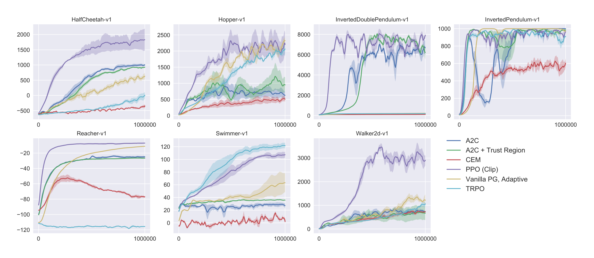
Key findings highlight PPO's strengths. First, the clipped objective achieved the highest average performance across the seven MuJoCo tasks, scoring 82% of the best possible normalized reward after tuning, compared to 76% or less for alternatives like adaptive penalties. Second, on those tasks, PPO outperformed established methods: it reached rewards about 20–50% higher than A2C or TRPO in environments like HalfCheetah and Hopper after one million steps. Third, PPO enabled a humanoid robot to learn running, steering toward targets, and recovering from falls under disturbances, achieving stable locomotion in 50–100 million steps. Fourth, on Atari games, PPO won 30 out of 49 in average episode rewards over training (versus 1 for A2C and 18 for ACER) and 19 in final performance, showing 10–50% better sample efficiency on many titles like Breakout and Qbert.

These results mean PPO delivers more reliable and efficient AI training, reducing the data and compute needed for high performance—potentially cutting costs and timelines for developing robotic or gaming systems by 20–40% compared to prior methods. It surprises by matching or exceeding complex trust-region techniques like TRPO while being far simpler, avoiding issues with noisy architectures or parameter sharing that plague others. This advances RL toward practical use in safety-critical areas, like autonomous vehicles, where robustness matters more than raw speed.

Leaders should prioritize PPO for new reinforcement learning projects, integrating it into frameworks like OpenAI Gym for initial pilots in simulation before real hardware. Trade-offs include slight hyperparameter tuning (e.g., clip range of 0.2), but it requires less adjustment than competitors. Next steps involve testing on diverse real-world data, such as physical robots or multi-agent scenarios, and combining PPO with experience replay for even better efficiency.

While experiments build confidence through multiple seeds and benchmarks, limitations include reliance on simulated environments, which may not fully capture real physics or noise, and sensitivity to initial hyperparameters. Results hold strongly for the tested domains, but caution applies to untested, high-variability tasks; further validation on larger scales would strengthen applicability.

1 Introduction

Section Summary: In recent years, researchers have developed various methods for training neural networks in reinforcement learning, including deep Q-learning, basic policy gradients, and trust region approaches, but each has drawbacks like poor scalability, inefficiency with data, or the need for extensive tuning. This paper introduces a new algorithm called PPO that matches the data efficiency and reliability of the more complex trust region method while using simpler optimization techniques, featuring a novel objective with clipped probability ratios to create a safe, lower-bound estimate of policy performance. Experiments show that PPO outperforms or simplifies previous methods on tasks like continuous control and Atari games, achieving better results with fewer samples.

In recent years, several different approaches have been proposed for reinforcement learning with neural network function approximators. The leading contenders are deep $Q$-learning [Mni+15], “vanilla” policy gradient methods [Mni+16], and trust region / natural policy gradient methods [Sch+15b]. However, there is room for improvement in developing a method that is scalable (to large models and parallel implementations), data efficient, and robust (i.e., successful on a variety of problems without hyperparameter tuning). $Q$-learning (with function approximation) fails on many simple problems[^1] and is poorly understood, vanilla policy gradient methods have poor data efficiency and robustness; and trust region policy optimization (TRPO) is relatively complicated, and is not compatible with architectures that include noise (such as dropout) or parameter sharing (between the policy and value function, or with auxiliary tasks).

This paper seeks to improve the current state of affairs by introducing an algorithm that attains the data efficiency and reliable performance of TRPO, while using only first-order optimization. We propose a novel objective with clipped probability ratios, which forms a pessimistic estimate (i.e., lower bound) of the performance of the policy. To optimize policies, we alternate between sampling data from the policy and performing several epochs of optimization on the sampled data.

Our experiments compare the performance of various different versions of the surrogate objective, and find that the version with the clipped probability ratios performs best. We also compare PPO to several previous algorithms from the literature. On continuous control tasks, it performs better than the algorithms we compare against. On Atari, it performs significantly better (in terms of sample complexity) than A2C and similarly to ACER though it is much simpler.

[^1]: While DQN works well on game environments like the Arcade Learning Environment [Bel+15] with discrete action spaces, it has not been demonstrated to perform well on continuous control benchmarks such as those in OpenAI Gym [Bro+16] and described by Duan et al. [Dua+16].

2 Background: Policy Optimization

Section Summary: Policy gradient methods in reinforcement learning improve decision-making policies by estimating how small changes to the policy affect performance, using sampled data to guide upward adjustments while weighting promising actions more heavily. These methods often rely on an objective function that can be optimized with standard tools, but repeatedly updating on the same data can cause unstable, overly large changes to the policy. Trust region methods, like TRPO, refine this by maximizing a similar objective but with a strict limit on how much the policy can deviate from its previous version, measured by a divergence metric, to ensure steady and reliable progress; while a penalty-based alternative exists in theory, practical constraints are preferred to avoid tuning issues across different scenarios.

2.1 Policy Gradient Methods

Policy gradient methods work by computing an estimator of the policy gradient and plugging it into a stochastic gradient ascent algorithm. The most commonly used gradient estimator has the form

$ \hat{g} = \hat{\mathbb{E}}t \left[ \nabla\theta \log \pi_\theta(a_t | s_t) \hat{A}_t \right]\tag{1} $

where $\pi_\theta$ is a stochastic policy and $\hat{A}_t$ is an estimator of the advantage function at timestep $t$. Here, the expectation $\hat{\mathbb{E}}_t[\dots]$ indicates the empirical average over a finite batch of samples, in an algorithm that alternates between sampling and optimization. Implementations that use automatic differentiation software work by constructing an objective function whose gradient is the policy gradient estimator; the estimator $\hat{g}$ is obtained by differentiating the objective

$ L^{PG}(\theta) = \hat{\mathbb{E}}t \left[ \log \pi\theta(a_t | s_t) \hat{A}_t \right].\tag{2} $

While it is appealing to perform multiple steps of optimization on this loss $L^{PG}$ using the same trajectory, doing so is not well-justified, and empirically it often leads to destructively large policy updates (see Section 6.1; results are not shown but were similar or worse than the “no clipping or penalty” setting).

2.2 Trust Region Methods

In TRPO [Sch+15b], an objective function (the “surrogate” objective) is maximized subject to a constraint on the size of the policy update. Specifically,

$ \underset{\theta}{\text{maximize}} \quad \hat{\mathbb{E}}t \left[ \frac{\pi\theta(a_t | s_t)}{\pi_{\theta_{\text{old}}}(a_t | s_t)} \hat{A}_t \right] \tag{3} $

$ \text{subject to} \quad \hat{\mathbb{E}}t \left[ \text{KL}[\pi{\theta_{\text{old}}}(\cdot | s_t), \pi_\theta(\cdot | s_t)] \right] \leq \delta. \tag{4} $

Here, $\theta_{\text{old}}$ is the vector of policy parameters before the update. This problem can efficiently be approximately solved using the conjugate gradient algorithm, after making a linear approximation to the objective and a quadratic approximation to the constraint.

The theory justifying TRPO actually suggests using a penalty instead of a constraint, i.e., solving the unconstrained optimization problem

$ \underset{\theta}{\text{maximize}} \ \hat{\mathbb{E}}t \left[ \frac{\pi\theta(a_t | s_t)}{\pi_{\theta_{\text{old}}}(a_t | s_t)} \hat{A}t - \beta \text{KL}[\pi{\theta_{\text{old}}}(\cdot | s_t), \pi_\theta(\cdot | s_t)] \right]\tag{5} $

for some coefficient $\beta$. This follows from the fact that a certain surrogate objective (which computes the max KL over states instead of the mean) forms a lower bound (i.e., a pessimistic bound) on the performance of the policy $\pi$. TRPO uses a hard constraint rather than a penalty because it is hard to choose a single value of $\beta$ that performs well across different problems—or even within a single problem, where the characteristics change over the course of learning. Hence, to achieve our goal of a first-order algorithm that emulates the monotonic improvement of TRPO, experiments show that it is not sufficient to simply choose a fixed penalty coefficient $\beta$ and optimize the penalized objective Equation (5) with SGD; additional modifications are required.

3 Clipped Surrogate Objective

Section Summary: The section discusses a surrogate objective in policy optimization called L^CPI, which encourages updates to an AI agent's decision-making policy by weighting actions based on their estimated benefits compared to an older version of the policy. To prevent overly drastic changes that could destabilize learning, the authors propose a modified "clipped" objective, L^CLIP, which limits how much the new policy can deviate from the old one by capping the influence of those benefits within a small range around the baseline. This clipping creates a conservative estimate that acts as a safety bound, ensuring updates are reliable without ignoring negative impacts, as illustrated in examples from control tasks.

Let $r_t(\theta)$ denote the probability ratio $r_t(\theta) = \frac{\pi_\theta(a_t | s_t)}{\pi_{\theta_{\text{old}}}(a_t | s_t)}$, so $r(\theta_{\text{old}}) = 1$. TRPO maximizes a “surrogate” objective

$ L^{CPI}(\theta) = \hat{\mathbb{E}}t \left[ \frac{\pi\theta(a_t | s_t)}{\pi_{\theta_{\text{old}}}(a_t | s_t)} \hat{A}_t \right] = \hat{\mathbb{E}}_t \left[ r_t(\theta) \hat{A}_t \right].\tag{6} $

The superscript $CPI$ refers to conservative policy iteration [KL02], where this objective was proposed. Without a constraint, maximization of $L^{CPI}$ would lead to an excessively large policy update; hence, we now consider how to modify the objective, to penalize changes to the policy that move $r_t(\theta)$ away from 1.

The main objective we propose is the following:

$ L^{CLIP}(\theta) = \hat{\mathbb{E}}_t \left[ \min(r_t(\theta) \hat{A}_t, \text{clip}(r_t(\theta), 1 - \epsilon, 1 + \epsilon) \hat{A}_t) \right]\tag{7} $

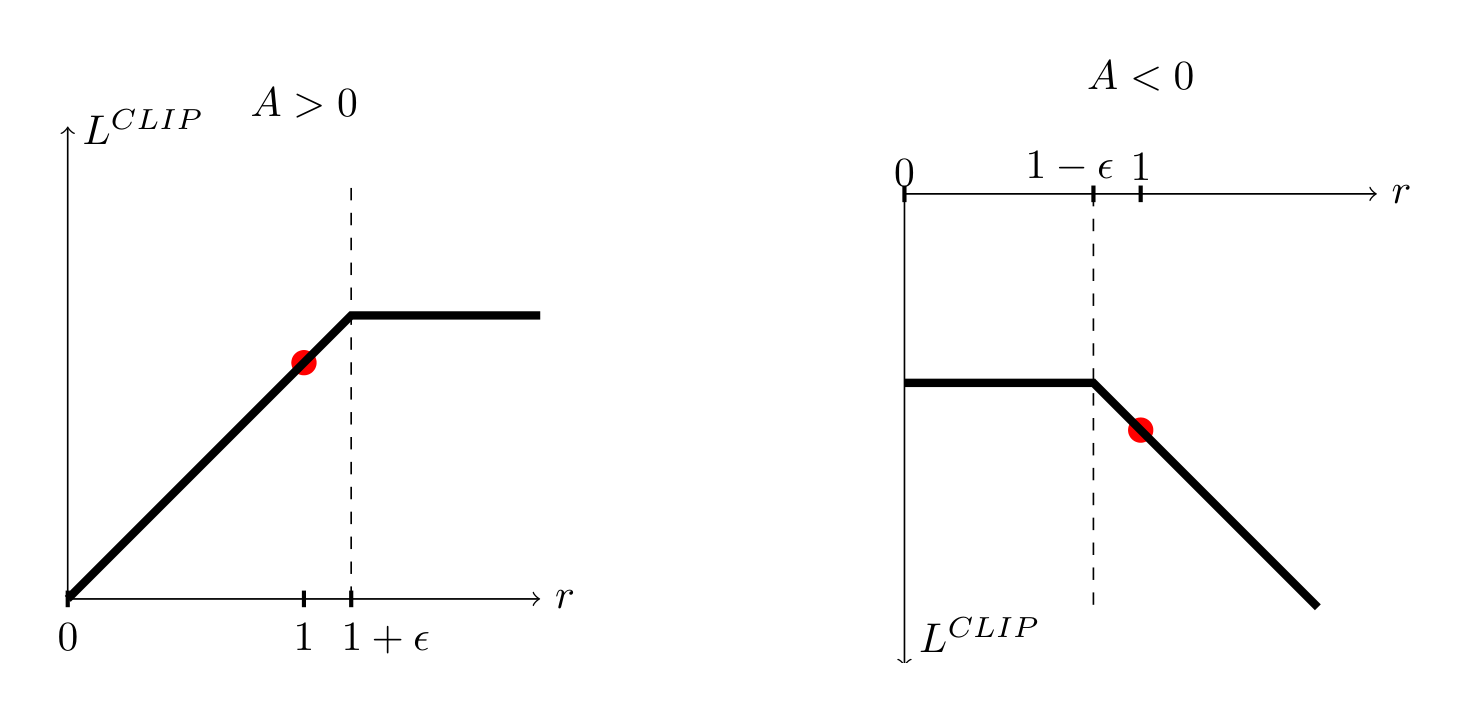
where $\epsilon$ is a hyperparameter, say $\epsilon = 0.2$. The motivation for this objective is as follows. The first term inside the min is $L^{CPI}$. The second term, $\text{clip}(r_t(\theta), 1 - \epsilon, 1 + \epsilon) \hat{A}t$, modifies the surrogate objective by clipping the probability ratio, which removes the incentive for moving $r_t$ outside of the interval $[1 - \epsilon, 1 + \epsilon]$. Finally, we take the minimum of the clipped and unclipped objective, so the final objective is a lower bound (i.e., a pessimistic bound) on the unclipped objective. With this scheme, we only ignore the change in probability ratio when it would make the objective improve, and we include it when it makes the objective worse. Note that $L^{CLIP}(\theta) = L^{CPI}(\theta)$ to first order around $\theta{\text{old}}$ (i.e., where $r = 1$), however, they become different as $\theta$ moves away from $\theta_{\text{old}}$. Figure 1 plots a single term (i.e., a single $t$) in $L^{CLIP}$; note that the probability ratio $r$ is clipped at $1 - \epsilon$ or $1 + \epsilon$ depending on whether the advantage is positive or negative.

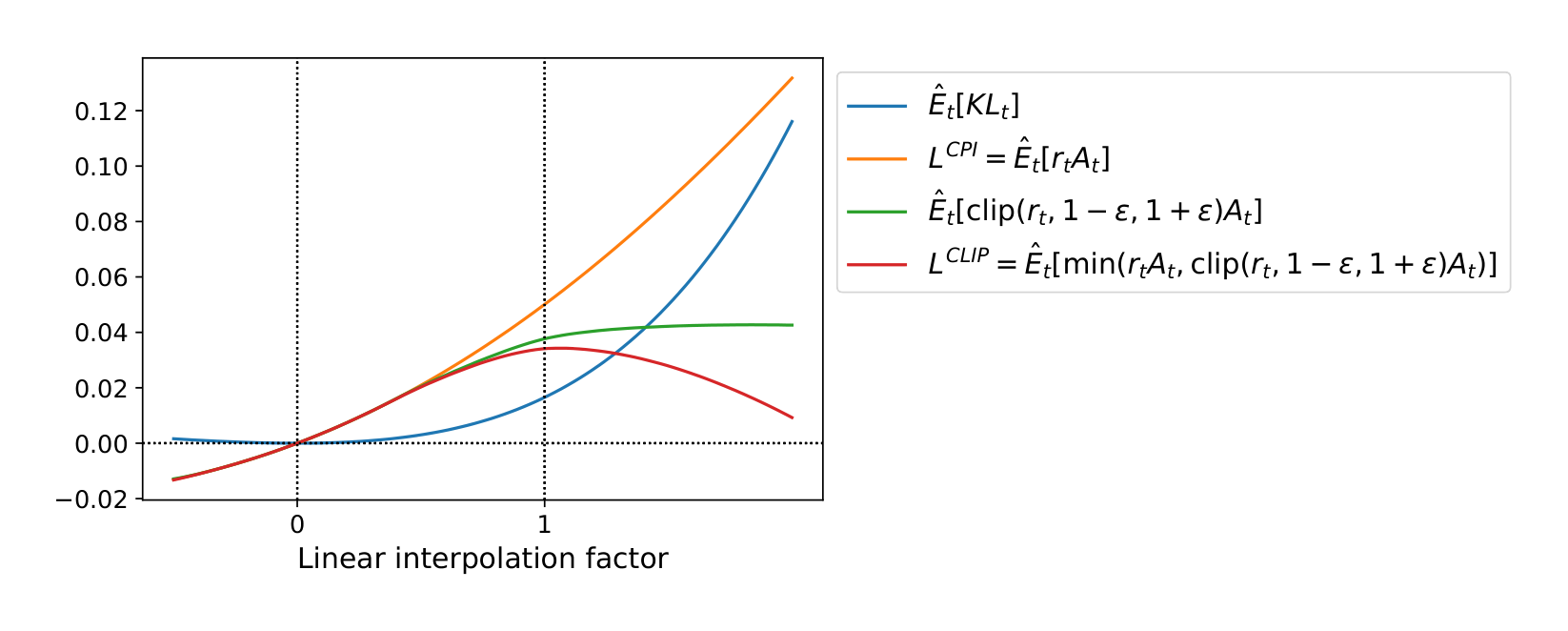
Figure 2 provides another source of intuition about the surrogate objective $L^{CLIP}$. It shows how several objectives vary as we interpolate along the policy update direction, obtained by proximal policy optimization (the algorithm we will introduce shortly) on a continuous control problem. We can see that $L^{CLIP}$ is a lower bound on $L^{CPI}$, with a penalty for having too large of a policy update.

4 Adaptive KL Penalty Coefficient

Section Summary: This method offers an alternative or supplement to the clipped surrogate objective by adding a penalty for KL divergence, which measures how much the new policy differs from the old one, and adjusts a penalty coefficient called beta to keep that divergence close to a target value during each policy update. In practice, it involves optimizing an objective function that includes the policy ratio and advantages minus the beta-weighted KL penalty using small batches of data, then checking the average KL divergence and halving beta if it's too low or doubling it if too high to refine the balance. Although experiments showed this approach underperformed compared to the clipped method, it's included as a useful baseline, with the adjustment scheme being robust and quick to stabilize despite occasional fluctuations.

Another approach, which can be used as an alternative to the clipped surrogate objective, or in addition to it, is to use a penalty on KL divergence, and to adapt the penalty coefficient so that we achieve some target value of the KL divergence $d_{\text{targ}}$ each policy update. In our experiments, we found that the KL penalty performed worse than the clipped surrogate objective, however, we’ve included it here because it’s an important baseline.

In the simplest instantiation of this algorithm, we perform the following steps in each policy update:

• Using several epochs of minibatch SGD, optimize the KL-penalized objective

$ L^{KLPEN}(\theta) = \hat{\mathbb{E}}t \left[ \frac{\pi\theta(a_t | s_t)}{\pi_{\theta_{\text{old}}}(a_t | s_t)} \hat{A}t - \beta \text{KL}[\pi{\theta_{\text{old}}}(\cdot | s_t), \pi_\theta(\cdot | s_t)] \right]\tag{8} $

• Compute $d = \hat{\mathbb{E}}t \left[ \text{KL}[\pi{\theta_{\text{old}}}(\cdot | s_t), \pi_\theta(\cdot | s_t)] \right]$ – If $d < d_{\text{targ}}/1.5, \beta \leftarrow \beta/2$ – If $d > d_{\text{targ}} \times 1.5, \beta \leftarrow \beta \times 2$

The updated $\beta$ is used for the next policy update. With this scheme, we occasionally see policy updates where the KL divergence is significantly different from $d_{\text{targ}}$, however, these are rare, and $\beta$ quickly adjusts. The parameters 1.5 and 2 above are chosen heuristically, but the algorithm is not very sensitive to them. The initial value of $\beta$ is another hyperparameter but is not important in practice because the algorithm quickly adjusts it.

5 Algorithm

Section Summary: This section explains how to implement advanced surrogate losses like CLIP or KLPEN in policy gradient methods by simply swapping them into existing setups and using automatic differentiation for optimization, often combined with a value function to reduce variance and an entropy bonus to encourage exploration. It details a combined objective that balances the policy update, value prediction accuracy, and randomness in actions. The described PPO algorithm uses parallel actors to gather short trajectories of experience, computes truncated advantage estimates for these segments, and then refines the policy through multiple epochs of stochastic gradient updates on the data.

The surrogate losses from the previous sections can be computed and differentiated with a minor change to a typical policy gradient implementation. For implementations that use automatic differentiation, one simply constructs the loss $L^{CLIP}$ or $L^{KLPEN}$ instead of $L^{PG}$, and one performs multiple steps of stochastic gradient ascent on this objective.

Most techniques for computing variance-reduced advantage-function estimators make use a learned state-value function $V(s)$; for example, generalized advantage estimation [Sch+15a], or the finite-horizon estimators in [Mni+16]. If using a neural network architecture that shares parameters between the policy and value function, we must use a loss function that combines the policy surrogate and a value function error term. This objective can further be augmented by adding an entropy bonus to ensure sufficient exploration, as suggested in past work [Wil92; Mni+16]. Combining these terms, we obtain the following objective, which is (approximately) maximized each iteration:

$ L^{CLIP+VF+S}_t(\theta) = \hat{\mathbb{E}}_t \left[ L^{CLIP}_t(\theta) - c_1 L^{VF}_t(\theta) + c_2 S\pi_\theta \right],\tag{9} $

where $c_1, c_2$ are coefficients, and $S$ denotes an entropy bonus, and $L^{VF}t$ is a squared-error loss $(V\theta(s_t) - V^{\text{targ}}_t)^2$.

One style of policy gradient implementation, popularized in [Mni+16] and well-suited for use with recurrent neural networks, runs the policy for $T$ timesteps (where $T$ is much less than the episode length), and uses the collected samples for an update. This style requires an advantage estimator that does not look beyond timestep $T$. The estimator used by [Mni+16] is

$ \hat{A}t = -V(s_t) + r_t + \gamma r{t+1} + \dots + \gamma^{T-t+1} r_{T-1} + \gamma^{T-t} V(s_T)\tag{10} $

where $t$ specifies the time index in $[0, T]$, within a given length-$T$ trajectory segment. Generalizing this choice, we can use a truncated version of generalized advantage estimation, which reduces to Equation (10) when $\lambda = 1$:

$ \hat{A}t = \delta_t + (\gamma\lambda)\delta{t+1} + \dots + (\gamma\lambda)^{T-t+1}\delta_{T-1},\tag{11} $

$ \text{where } \delta_t = r_t + \gamma V(s_{t+1}) - V(s_t)\tag{12} $

A proximal policy optimization (PPO) algorithm that uses fixed-length trajectory segments is shown below. Each iteration, each of $N$ (parallel) actors collect $T$ timesteps of data. Then we construct the surrogate loss on these $NT$ timesteps of data, and optimize it with minibatch SGD (or usually for better performance, Adam [KB14]), for $K$ epochs.

Algorithm 1 PPO, Actor-Critic Style
for iteration=1, 2, . . . do
  for actor=1, 2, . . . , N do
    Run policy $\pi_{\theta_{\text{old}}}$ in environment for $T$ timesteps
    Compute advantage estimates $\hat{A}_1, \dots, \hat{A}_T$
  end for
  Optimize surrogate $L$ wrt $\theta$, with $K$ epochs and minibatch size $M \leq NT$
  $\theta_{\text{old}} \leftarrow \theta$
end for

6 Experiments

Section Summary: The experiments section evaluates different versions of the Proximal Policy Optimization (PPO) algorithm on simulated robotics tasks using environments like OpenAI Gym and MuJoCo physics. It first compares surrogate objectives, finding that a clipped version with a specific parameter setting performs best across seven tasks, outperforming options without clipping or with KL penalties. PPO is then shown to surpass other established methods in continuous control problems, and as a highlight, it successfully trains a 3D humanoid robot to run, steer toward targets, recover from falls, and handle obstacles in more challenging scenarios.

6.1 Comparison of Surrogate Objectives

First, we compare several different surrogate objectives under different hyperparameters. Here, we compare the surrogate objective $L^{CLIP}$ to several natural variations and ablated versions.

No clipping or penalty: $L_t(\theta) = r_t(\theta) \hat{A}_t$
Clipping: $L_t(\theta) = \min(r_t(\theta) \hat{A}t, \text{clip}(r_t(\theta), 1 - \epsilon, 1 + \epsilon) \hat{A}t)$
KL penalty (fixed or adaptive) $L_t(\theta) = r_t(\theta) \hat{A}t - \beta \text{KL}[\pi{\theta{\text{old}}}, \pi\theta]$

For the KL penalty, one can either use a fixed penalty coefficient $\beta$ or an adaptive coefficient as described in Section 4 using target KL value $d_{\text{targ}}$. Note that we also tried clipping in log space, but found the performance to be no better.

Because we are searching over hyperparameters for each algorithm variant, we chose a computationally cheap benchmark to test the algorithms on. Namely, we used 7 simulated robotics tasks[^2] implemented in OpenAI Gym [Bro+16], which use the MuJoCo [TET12] physics engine. We do one million timesteps of training on each one. Besides the hyperparameters used for clipping ($\epsilon$) and the KL penalty ($\beta, d_{\text{targ}}$), which we search over, the other hyperparameters are provided in Table 3.

To represent the policy, we used a fully-connected MLP with two hidden layers of 64 units, and tanh nonlinearities, outputting the mean of a Gaussian distribution, with variable standard deviations, following [Sch+15b; Dua+16]. We don’t share parameters between the policy and value function (so coefficient $c_1$ is irrelevant), and we don’t use an entropy bonus.

Each algorithm was run on all 7 environments, with 3 random seeds on each. We scored each run of the algorithm by computing the average total reward of the last 100 episodes. We shifted and scaled the scores for each environment so that the random policy gave a score of 0 and the best result was set to 1, and averaged over 21 runs to produce a single scalar for each algorithm setting.

The results are shown in Table 1. Note that the score is negative for the setting without clipping or penalties, because for one environment (half cheetah) it leads to a very negative score, which is worse than the initial random policy.

: Table 1: Results from continuous control benchmark. Average normalized scores (over 21 runs of the algorithm, on 7 environments) for each algorithm / hyperparameter setting . $\beta$ was initialized at 1.

\begin{tabular}{lc}
\hline
algorithm & avg. normalized score \\
\hline
No clipping or penalty & -0.39 \\
Clipping, $\epsilon = 0.1$ & 0.76 \\
\textbf{Clipping, $\epsilon = 0.2$} & \textbf{0.82} \\
Clipping, $\epsilon = 0.3$ & 0.70 \\
Adaptive KL $d_{\text{targ}} = 0.003$ & 0.68 \\
Adaptive KL $d_{\text{targ}} = 0.01$ & 0.74 \\
Adaptive KL $d_{\text{targ}} = 0.03$ & 0.71 \\
Fixed KL, $\beta = 0.3$ & 0.62 \\
Fixed KL, $\beta = 1.$ & 0.71 \\
Fixed KL, $\beta = 3.$ & 0.72 \\
Fixed KL, $\beta = 10.$ & 0.69 \\
\hline
\end{tabular}

[^2]: HalfCheetah, Hopper, InvertedDoublePendulum, InvertedPendulum, Reacher, Swimmer, and Walker2d, all “-v1”

6.2 Comparison to Other Algorithms in the Continuous Domain

Next, we compare PPO (with the “clipped” surrogate objective from Section 3) to several other methods from the literature, which are considered to be effective for continuous problems. We compared against tuned implementations of the following algorithms: trust region policy optimization [Sch+15b], cross-entropy method (CEM) [SL06], vanilla policy gradient with adaptive stepsize[^3], A2C [Mni+16], A2C with trust region [Wan+16]. A2C stands for advantage actor critic, and is a synchronous version of A3C, which we found to have the same or better performance than the asynchronous version. For PPO, we used the hyperparameters from the previous section, with $\epsilon = 0.2$. We see that PPO outperforms the previous methods on almost all the continuous control environments.

[^3]: After each batch of data, the Adam stepsize is adjusted based on the KL divergence of the original and updated policy, using a rule similar to the one shown in Section 4. An implementation is available at https://github.com/berkeleydeeprlcourse/homework/tree/master/hw4.

6.3 Showcase in the Continuous Domain: Humanoid Running and Steering

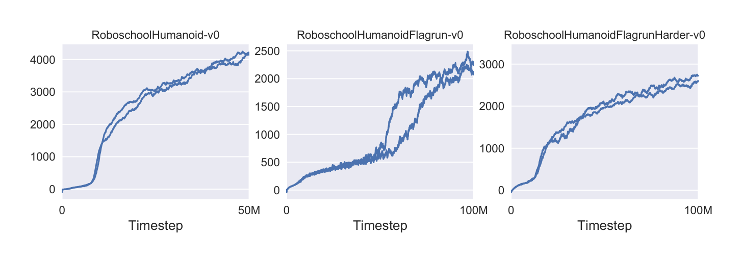
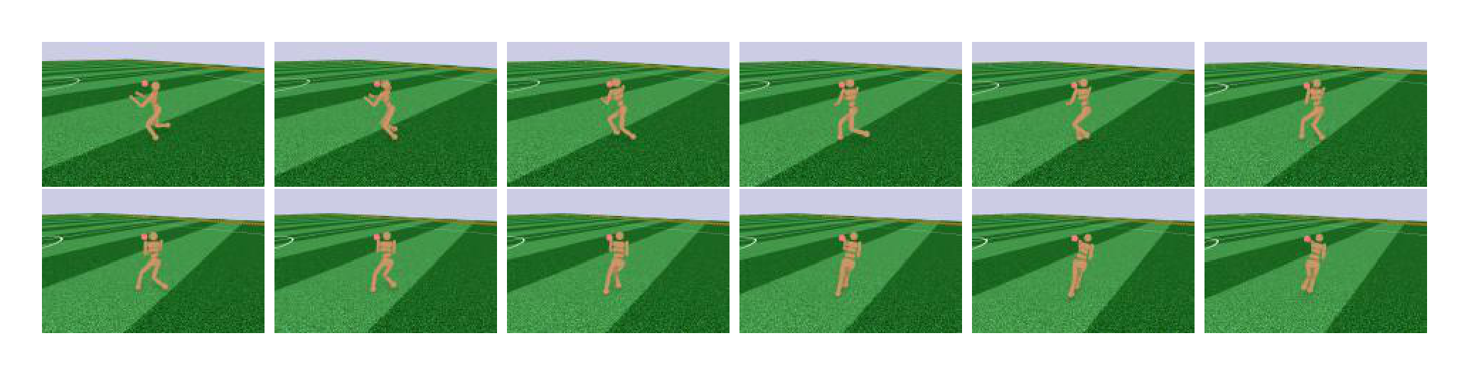
To showcase the performance of PPO on high-dimensional continuous control problems, we train on a set of problems involving a 3D humanoid, where the robot must run, steer, and get up off the ground, possibly while being pelted by cubes. The three tasks we test on are (1) RoboschoolHumanoid: forward locomotion only, (2) RoboschoolHumanoidFlagrun: position of target is randomly varied every 200 timesteps or whenever the goal is reached, (3) RoboschoolHumanoidFlagrunHarder, where the robot is pelted by cubes and needs to get up off the ground. See Figure 5 for still frames of a learned policy, and Figure 4 for learning curves on the three tasks. Hyperparameters are provided in Table 4. In concurrent work, Heess et al. [Hee+17] used the adaptive KL variant of PPO (Section 4) to learn locomotion policies for 3D robots.

6.4 Comparison to Other Algorithms on the Atari Domain

We also ran PPO on the Arcade Learning Environment [Bel+15] benchmark and compared against well-tuned implementations of A2C [Mni+16] and ACER [Wan+16]. For all three algorithms, we used the same policy network architecture as used in [Mni+16]. The hyperparameters for PPO are provided in Table 5. For the other two algorithms, we used hyperparameters that were tuned to maximize performance on this benchmark.

A table of results and learning curves for all 49 games is provided in Appendix B. We consider the following two scoring metrics: (1) average reward per episode over entire training period (which favors fast learning), and (2) average reward per episode over last 100 episodes of training (which favors final performance). Table 2 shows the number of games “won” by each algorithm, where we compute the victor by averaging the scoring metric across three trials.

: Table 2: Number of games “won” by each algorithm, where the scoring metric is averaged across three trials.

\begin{tabular}{lrrrr}
\hline
& A2C & ACER & PPO & Tie \\
\hline
(1) avg. episode reward over all of training & 1 & 18 & \textbf{30} & 0 \\
(2) avg. episode reward over last 100 episodes & 1 & \textbf{28} & 19 & 1 \\
\hline
\end{tabular}

7 Conclusion

Section Summary: Proximal policy optimization is a new set of techniques for improving AI decision-making strategies through repeated small updates using a common optimization approach. These methods offer the same steady and dependable results as more complex trust-region techniques but are far easier to put into practice, needing only minor tweaks to basic existing code. They work well in broader scenarios, like when combining policy and evaluation components, and deliver superior results overall.

We have introduced proximal policy optimization, a family of policy optimization methods that use multiple epochs of stochastic gradient ascent to perform each policy update. These methods have the stability and reliability of trust-region methods but are much simpler to implement, requiring only few lines of code change to a vanilla policy gradient implementation, applicable in more general settings (for example, when using a joint architecture for the policy and value function), and have better overall performance.

8 Acknowledgements

Thanks to Rocky Duan, Peter Chen, and others at OpenAI for insightful comments.

References

Section Summary: This section lists key research papers on reinforcement learning and artificial intelligence, focusing on tools and methods for training AI agents in games, simulations, and physical tasks. It includes influential works like those introducing environments such as OpenAI Gym and the Arcade Learning Environment for testing AI performance, as well as algorithms for optimization, deep learning control, and behaviors like locomotion. The references span from 1992 to 2017, highlighting foundational advances by researchers at institutions like DeepMind and OpenAI.

[Bel+15] M. Bellemare, Y. Naddaf, J. Veness, and M. Bowling. “The arcade learning environment: An evaluation platform for general agents”. In: Twenty-Fourth International Joint Conference on Artificial Intelligence. 2015.

[Bro+16] G. Brockman, V. Cheung, L. Pettersson, J. Schneider, J. Schulman, J. Tang, and W. Zaremba. “OpenAI Gym”. In: arXiv preprint arXiv:1606.01540 (2016).

[Dua+16] Y. Duan, X. Chen, R. Houthooft, J. Schulman, and P. Abbeel. “Benchmarking Deep Reinforcement Learning for Continuous Control”. In: arXiv preprint arXiv:1604.06778 (2016).

[Hee+17] N. Heess, S. Sriram, J. Lemmon, J. Merel, G. Wayne, Y. Tassa, T. Erez, Z. Wang, A. Eslami, M. Riedmiller, et al. “Emergence of Locomotion Behaviours in Rich Environments”. In: arXiv preprint arXiv:1707.02286 (2017).

[KL02] S. Kakade and J. Langford. “Approximately optimal approximate reinforcement learning”. In: ICML. Vol. 2. 2002, pp. 267–274.

[KB14] D. Kingma and J. Ba. “Adam: A method for stochastic optimization”. In: arXiv preprint arXiv:1412.6980 (2014).

[Mni+15] V. Mnih, K. Kavukcuoglu, D. Silver, A. A. Rusu, J. Veness, M. G. Bellemare, A. Graves, M. Riedmiller, A. K. Fidjeland, G. Ostrovski, et al. “Human-level control through deep reinforcement learning”. In: Nature 518.7540 (2015), pp. 529–533.

[Mni+16] V. Mnih, A. P. Badia, M. Mirza, A. Graves, T. P. Lillicrap, T. Harley, D. Silver, and K. Kavukcuoglu. “Asynchronous methods for deep reinforcement learning”. In: arXiv preprint arXiv:1602.01783 (2016).

[Sch+15a] J. Schulman, P. Moritz, S. Levine, M. Jordan, and P. Abbeel. “High-dimensional continuous control using generalized advantage estimation”. In: arXiv preprint arXiv:1506.02438 (2015).

[Sch+15b] J. Schulman, S. Levine, P. Moritz, M. I. Jordan, and P. Abbeel. “Trust region policy optimization”. In: CoRR, abs/1502.05477 (2015).

[SL06] I. Szita and A. Lörincz. “Learning Tetris using the noisy cross-entropy method”. In: Neural computation 18.12 (2006), pp. 2936–2941.

[TET12] E. Todorov, T. Erez, and Y. Tassa. “MuJoCo: A physics engine for model-based control”. In: Intelligent Robots and Systems (IROS), 2012 IEEE/RSJ International Conference on. IEEE. 2012, pp. 5026–5033.

[Wan+16] Z. Wang, V. Bapst, N. Heess, V. Mnih, R. Munos, K. Kavukcuoglu, and N. de Freitas. “Sample Efficient Actor-Critic with Experience Replay”. In: arXiv preprint arXiv:1611.01224 (2016).

[Wil92] R. J. Williams. “Simple statistical gradient-following algorithms for connectionist reinforcement learning”. In: Machine learning 8.3-4 (1992), pp. 229–256.

A Hyperparameters

Section Summary: This section details the key settings, or hyperparameters, used in the PPO reinforcement learning algorithm across different experiments. For the Mujoco benchmark, it lists parameters like a 2048-step horizon, a learning rate of 0.0003, and 10 training epochs per batch. The Roboschool experiments adjust the learning rate based on divergence targets and use a shorter 512-step horizon with varying actor counts, while the Atari setup employs a 128-step horizon, scaled learning rates that decrease over time, and additional coefficients for value and entropy to guide the training process.

: Table 3: PPO hyperparameters used for the Mujoco 1 million timestep benchmark.

\begin{tabular}{l|l}
Hyperparameter & Value \\
\hline
Horizon (T) & 2048 \\
Adam stepsize & $3 \times 10^{-4}$ \\
Num. epochs & 10 \\
Minibatch size & 64 \\
Discount ($\gamma$) & 0.99 \\
GAE parameter ($\lambda$) & 0.95 \\
\end{tabular}

: Table 4: PPO hyperparameters used for the Roboschool experiments. Adam stepsize was adjusted based on the target value of the KL divergence.

\begin{tabular}{l|l}
Hyperparameter & Value \\
\hline
Horizon (T) & 512 \\
Adam stepsize & * \\
Num. epochs & 15 \\
Minibatch size & 4096 \\
Discount ($\gamma$) & 0.99 \\
GAE parameter ($\lambda$) & 0.95 \\
Number of actors & 32 (locomotion), 128 (flagrun) \\
Log stdev. of action distribution & LinearAnneal(-0.7, -1.6) \\
\end{tabular}

: Table 5: PPO hyperparameters used in Atari experiments. $\alpha$ is linearly annealed from 1 to 0 over the course of learning.

\begin{tabular}{l|l}
Hyperparameter & Value \\
\hline
Horizon (T) & 128 \\
Adam stepsize & $2.5 \times 10^{-4} \times \alpha$ \\
Num. epochs & 3 \\
Minibatch size & $32 \times 8$ \\
Discount ($\gamma$) & 0.99 \\
GAE parameter ($\lambda$) & 0.95 \\
Number of actors & 8 \\
Clipping parameter $\epsilon$ & $0.1 \times \alpha$ \\
VF coeff. $c_1$ (9) & 1 \\
Entropy coeff. $c_2$ (9) & 0.01 \\
\end{tabular}

B Performance on More Atari Games

Section Summary: This section compares the reinforcement learning algorithm PPO with A2C and ACER across 49 classic Atari video games from OpenAI Gym. A figure shows how each algorithm's performance improves over time across three different random starts, while a table lists their average final scores after millions of gameplay frames. PPO achieves the highest scores in over half the games, such as Assault and Atlantis, highlighting its strong overall performance compared to the others.

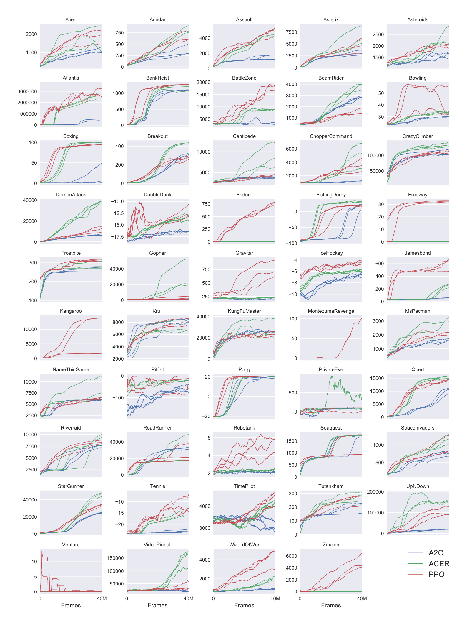
Here we include a comparison of PPO against A2C on a larger collection of 49 Atari games. Figure 6 shows the learning curves of each of three random seeds, while Table 6 shows the mean performance.

: Table 6: Mean final scores (last 100 episodes) of PPO and A2C on Atari games after 40M game frames (10M timesteps).

\begin{tabular}{lrrr}
\hline
& A2C & ACER & PPO \\
\hline
Alien & 1141.7 & 1655.4 & \textbf{1850.3} \\
Amidar & 380.8 & \textbf{827.6} & 674.6 \\
Assault & 1562.9 & 4653.8 & \textbf{4971.9} \\
Asterix & 3176.3 & \textbf{6801.2} & 4532.5 \\
Asteroids & 1653.3 & \textbf{2389.3} & 2097.5 \\
Atlantis & 729265.3 & 1841376.0 & \textbf{2311815.0} \\
BankHeist & 1095.3 & 1177.5 & \textbf{1280.6} \\
BattleZone & 3080.0 & 8983.3 & \textbf{17366.7} \\
BeamRider & 3031.7 & \textbf{3863.3} & 1590.0 \\
Bowling & 30.1 & 33.3 & \textbf{40.1} \\
Boxing & 17.7 & \textbf{98.9} & 94.6 \\
Breakout & 303.0 & \textbf{456.4} & 274.8 \\
Centipede & 3496.5 & \textbf{8904.8} & 4386.4 \\
ChopperCommand & 1171.7 & \textbf{5287.7} & 3516.3 \\
CrazyClimber & 107770.0 & \textbf{132461.0} & 110202.0 \\
DemonAttack & 6639.1 & \textbf{38808.3} & 11378.4 \\
DoubleDunk & -16.2 & \textbf{-13.2} & -14.9 \\
Enduro & 0.0 & 0.0 & \textbf{758.3} \\
FishingDerby & 20.6 & \textbf{34.7} & 17.8 \\
Freeway & 0.0 & 0.0 & \textbf{32.5} \\
Frostbite & 261.8 & 285.6 & \textbf{314.2} \\
Gopher & 1500.9 & \textbf{37802.3} & 2932.9 \\
Gravitar & 194.0 & 225.3 & \textbf{737.2} \\
IceHockey & -6.4 & -5.9 & \textbf{-4.2} \\
Jamesbond & 52.3 & 261.8 & \textbf{560.7} \\
Kangaroo & 45.3 & 50.0 & \textbf{9928.7} \\
Krull & \textbf{8367.4} & 7268.4 & 7942.3 \\
KungFuMaster & 24900.3 & \textbf{27599.3} & 23310.3 \\
MontezumaRevenge & 0.0 & 0.3 & \textbf{42.0} \\
MsPacman & 1626.9 & \textbf{2718.5} & 2096.5 \\
NameThisGame & 5961.2 & \textbf{8488.0} & 6254.9 \\
Pitfall & -55.0 & \textbf{-16.9} & -32.9 \\
Pong & 19.7 & \textbf{20.7} & \textbf{20.7} \\
PrivateEye & 91.3 & \textbf{182.0} & 69.5 \\
Qbert & 10065.7 & \textbf{15316.6} & 14293.3 \\
Riverraid & 7653.5 & \textbf{9125.1} & 8393.6 \\
RoadRunner & 32810.0 & \textbf{35466.0} & 25076.0 \\
Robotank & 2.2 & 2.5 & \textbf{5.5} \\
Seaquest & 1714.3 & \textbf{1739.5} & 1204.5 \\
SpaceInvaders & 744.5 & \textbf{1213.9} & 942.5 \\
StarGunner & 26204.0 & \textbf{49817.7} & 32689.0 \\
Tennis & -22.2 & -17.6 & \textbf{-14.8} \\
TimePilot & 2898.0 & 4175.7 & \textbf{4342.0} \\
Tutankham & 206.8 & \textbf{280.8} & 254.4 \\
UpNDown & 17369.8 & \textbf{145051.4} & 95445.0 \\
Venture & 0.0 & 0.0 & 0.0 \\
VideoPinball & 19735.9 & \textbf{156225.6} & 37389.0 \\
WizardOfWor & 859.0 & 2308.3 & \textbf{4185.3} \\
Zaxxon & 16.3 & 29.0 & \textbf{5008.7} \\
\hline
\end{tabular}