Matching with PROSAC - progressive sample consensus

Ondřej ChumJiri Matas

article2005CVPR1,363 citations

Proposes a sample consensus algorithm that accelerates correspondence matching by orders of magnitude over RANSAC through progressive sampling of tentative matches ordered by similarity, while retaining identical worst-case convergence guarantees.

Listen

Reliable feature matching between multiple images is a foundational requirement in computer vision tasks such as 3D reconstruction, stereo matching, and motion tracking. Traditional pipelines use standard random sample consensus (RANSAC) to filter out incorrect matches (outliers) from correct geometric alignments (inliers). However, standard RANSAC treats all candidate correspondences as equally probable, drawing samples uniformly across the entire dataset. When images contain large fractions of outliers caused by occlusions, texture repetition, or significant viewpoint changes, standard random sampling becomes prohibitively slow and computationally expensive.

The article evaluates Progressive Sample Consensus (PROSAC), a robust estimation method designed to dramatically accelerate geometric model fitting. The main objective is to demonstrate that sampling candidate matches in order of their initial descriptor similarity yields massive speedups while maintaining the same statistical reliability guarantees as standard RANSAC.

To establish its findings, the article evaluates PROSAC across challenging wide-baseline image pairs featuring repetitive patterns, depth discontinuities, occlusions, and independent foreground motions. The approach uses existing local similarity measures (such as SIFT descriptor ratios and transform coefficient distances) to order correspondences from highest to lowest quality. Instead of sampling uniformly, PROSAC samples from progressively larger subsets of the top-ranked candidates, dynamically balancing early deterministic testing of high-quality matches with gradual convergence toward standard uniform sampling. The experiments compare sample counts and wall-clock execution times across benchmark scenes against traditional RANSAC.

The analysis reveals three key findings. First, the foundational assumption that match similarity predicts true correctness better than random guessing held across all tested datasets, with inlier concentration declining steadily toward lower-ranked matches. Second, PROSAC delivered substantial speed improvements—often reducing computation time by a factor of 100 or more. In one benchmark scene, PROSAC required an average of 9 samples (0.06 seconds) to resolve the geometric model compared to 106,534 samples (10.76 seconds) for RANSAC. Third, PROSAC successfully recovered geometric alignments in extreme noise environments where RANSAC failed completely, such as a scene requiring an estimated 84 million RANSAC trials that PROSAC resolved in 3,576 samples (0.76 seconds).

These findings have significant practical implications for real-time computer vision systems, motion segmentation, and autonomous tracking pipelines. By finding valid models early within high-confidence subsets, PROSAC substantially reduces latency, computational cost, and hardware resource demands. Furthermore, it eliminates the operational burden of manually fine-tuning conservative similarity thresholds, making computer vision pipelines significantly more robust against noisy or sparse candidate pools.

Organizations developing feature matching and multi-view vision systems should adopt PROSAC in place of standard RANSAC for geometric model estimation. When integrating the method, developers can safely relax initial feature-filtering thresholds to capture more true matches without risking catastrophic performance degradation from added outliers.

Confidence in these results is high, as PROSAC mathematically converges to standard RANSAC in worst-case scenarios where similarity ordering is purely random. Tests using randomly permuted data confirmed that PROSAC maintains performance at or slightly above RANSAC even when quality rankings provide zero predictive value. However, users should note that the speed advantage diminishes if local similarity metrics fail to correlate with correct matches, such as in scenes dominated by extreme repetitive textures or independent foreground motions that share high visual similarity.

  • Paper: Distinctive Image Features from Scale-Invariant Keypoints, David G. Lowe (2004). It introduces the SIFT feature detector and descriptor, whose similarity metric and nearest-neighbor distance ratios provide the foundational sorting order that PROSAC exploits for prioritized sampling.
  • Paper: An efficient solution to the five-point relative pose problem, David Nister (2004). It establishes the efficient minimal 5-point relative pose solver used within robust hypothesis generation pipelines that PROSAC accelerates.
  • Paper: In Defense of the Eight-Point Algorithm, Richard I. Hartley (1997). It provides the normalized eight-point algorithm for estimating epipolar geometry and fundamental matrices, serving as a classical geometric model fitted during robust sample consensus.
  • Paper: Scale & Affine Invariant Interest Point Detectors, Krystian Mikolajczyk et al. (2004). It details scale- and affine-invariant interest point detectors that provide the candidate visual correspondences necessary for wide-baseline geometric model estimation.
  • Paper: Evaluation of Interest Point Detectors, CORDELIA SCHMID et al. (2000). It establishes foundational criteria for measuring feature detector repeatability and distinctiveness across varying viewpoints prior to geometric correspondence matching.
Cover for Matching with PROSAC - progressive sample consensus

Abstract

A new robust matching method is proposed. The Progressive Sample Consensus (PROSAC) algorithm exploits the linear ordering defined on the set of correspondences by a similarity function used in establishing tentative correspondences. Unlike RANSAC, which treats all correspondences equally and draws random samples uniformly from the full set, PROSAC samples are drawn from progressively larger sets of top-ranked correspondences.

Under the mild assumption that the similarity measure predicts correctness of a match better than random guessing, we show that PROSAC achieves large computational savings. Experiments demonstrate it is often significantly faster (up to more than hundred times) than RANSAC.

For the derived size of the sampled set of correspondences as a function of the number of samples already drawn, PROSAC converges towards RANSAC in the worst case. The power of the method is demonstrated on wide-baseline matching problems.

Table of Contents

  • 1. Introduction
  • 1.1. Notation
  • 2. Algorithm
  • 2.1. The growth function and sampling
  • 2.2. Stopping criterion
  • 3. Experiments
  • 4. Conclusions
  • References

Knowls

  1. Knowl 1 — Progressive Sampling Scheme and Growth Function

    model/method

    Let UN={u1,u2,…,uN}U_N = \{u_1, u_2, \dots, u_N\} be a set of NN tentative point correspondences sorted in descending order according to a quality metric q(u)q(u), such that i<j  ⟹  q(ui)≥q(uj)i < j \implies q(u_i) \ge q(u_j). Let Un={u1,…,un}U_n = \{u_1, \dots, u_n\} denote the subset of the nn highest-ranked correspondences, and let mm be the minimal sample size required to estimate the geometric model parameters.

    Assume a standard RANSAC procedure draws TNT_N samples of size mm uniformly from UNU_N. The expected number of these TNT_N samples that contain correspondences drawn exclusively from the top nn points UnU_n is:

    Tn=TN(nm)(Nm)=TN∏i=0m−1n−iN−iT_n = T_N \frac{\binom{n}{m}}{\binom{N}{m}} = T_N \prod_{i=0}^{m-1} \frac{n-i}{N-i}

    This yields the recurrent relation for successive sample counts:

    Tn+1=n+1n+1−mTnT_{n+1} = \frac{n+1}{n+1-m} T_n

    To ensure an integer progression of samples, discrete sample thresholds Tn′T'_n are initialized with Tm′=1T'_m = 1 and updated recursively by:

    Tn+1′=Tn′+⌈Tn+1−Tn⌉T'_{n+1} = T'_n + \lceil T_{n+1} - T_n \rceil

    The growth function g(t)g(t), which specifies the size of the active correspondence pool at trial tt, is defined as:

    g(t)=min⁡{n:Tn′≥t}g(t) = \min \{ n : T'_n \ge t \}

    At the tt-th sampling step, PROSAC draws the sample MtM_t by including the newest correspondence ug(t)u_{g(t)} together with m−1m-1 correspondences chosen uniformly at random from the prefix set Ug(t)−1U_{g(t)-1}:

    Mt={ug(t)}∪Mt′,Mt′⊂Ug(t)−1,  ∣Mt′∣=m−1M_t = \{u_{g(t)}\} \cup M'_t, \quad M'_t \subset U_{g(t)-1}, \; |M'_t| = m-1

    When t>TN′t > T'_N, PROSAC draws mm correspondences uniformly at random from UNU_N, matching the sampling distribution of standard RANSAC.

  2. Knowl 2 — Progressive Sample Consensus (PROSAC) Algorithm

    algorithm

    The Progressive Sample Consensus (PROSAC) algorithm estimates geometric model parameters from a quality-ordered set of tentative correspondences by drawing minimal samples from progressively expanding subsets of top-ranked matches.

    Input: Ordered tentative correspondences UN={u1,…,uN}U_N = \{u_1, \dots, u_N\} sorted by quality q(ui)≥q(ui+1)q(u_i) \ge q(u_{i+1}), minimal sample size mm, total nominal RANSAC samples TNT_N, confidence threshold η0\eta_0, non-randomness threshold Ψ\Psi, outlier support probability β\beta.
    Output: Optimal model parameters p∗p^* and associated inlier support S∗S^*.
    t←0t \leftarrow 0
    n←mn \leftarrow m
    n∗←Nn^* \leftarrow N
    Tn′←1T'_n \leftarrow 1
    kn∗(η0)←∞k_{n^*}(\eta_0) \leftarrow \infty
    S∗←∅S^* \leftarrow \emptyset
    repeat
        t←t+1t \leftarrow t + 1
        if t=Tn′t = T'_n and n<n∗n < n^* then
            n←n+1n \leftarrow n + 1
            Compute Tn=TN∏i=0m−1n−iN−iT_n = T_N \prod_{i=0}^{m-1} \frac{n-i}{N-i}
            Tn′←Tn−1′+⌈Tn−Tn−1⌉T'_n \leftarrow T'_{n-1} + \lceil T_n - T_{n-1} \rceil
        end if
        if t≤Tn′t \le T'_n then
            Draw Mt′⊂Un−1M'_t \subset U_{n-1} of size m−1m-1 uniformly at random
            Mt←{un}∪Mt′M_t \leftarrow \{u_n\} \cup M'_t
        else
            Draw Mt⊂UnM_t \subset U_n of size mm uniformly at random
        end if
        Compute model parameters ptp_t from sample MtM_t
        Find support set St⊂UNS_t \subset U_N of correspondences consistent with ptp_t
        if ∣St∣>∣S∗∣|S_t| > |S^*| then
            S∗←StS^* \leftarrow S_t
            p∗←ptp^* \leftarrow p_t
            
            for each n′∈{m,…,N}n' \in \{m, \dots, N\} do
                In′←∣St∩Un′∣I_{n'} \leftarrow |S_t \cap U_{n'}|
                Compute In′min⁡=min⁡{j:∑i=jn′Pn′R(i)<Ψ}I_{n'}^{\min} = \min \{ j : \sum_{i=j}^{n'} P_{n'}^R(i) < \Psi \}
                if In′≥In′min⁡I_{n'} \ge I_{n'}^{\min} then
                    PIn′←∏j=0m−1In′−jn′−jP_{I_{n'}} \leftarrow \prod_{j=0}^{m-1} \frac{I_{n'} - j}{n' - j}
                    kn′←log⁡(η0)log⁡(1−PIn′)k_{n'} \leftarrow \frac{\log(\eta_0)}{\log(1 - P_{I_{n'}})}
                    if kn′<kn∗(η0)k_{n'} < k_{n^*}(\eta_0) then
                        kn∗(η0)←kn′k_{n^*}(\eta_0) \leftarrow k_{n'}
                        n∗←n′n^* \leftarrow n'
                    end if
                end if
            end for
        end if
    until t≥kn∗(η0)t \ge k_{n^*}(\eta_0) and ∣S∗∩Un∗∣≥In∗min⁡|S^* \cap U_{n^*}| \ge I_{n^*}^{\min}
    return p∗,S∗p^*, S^*

    PROSAC terminates when the drawn sample count tt meets the sample requirement kn∗(η0)k_{n^*}(\eta_0) and the non-randomness support bound is satisfied on the optimal subset Un∗U_{n^*}. Typical hyperparameter settings are TN=200000T_N = 200000 and η0=Ψ=0.05\eta_0 = \Psi = 0.05.

  3. Knowl 3 — Non-Randomness Stopping Criterion

    equation

    To prevent terminating on an incorrect model supported by random alignments of outliers, PROSAC enforces a non-randomness condition. The distribution of the number of correspondences ii out of nn tentative correspondences that by chance support an incorrect model generated from a minimal sample of size mm follows a binomial distribution:

    PnR(i)=βi−m(1−β)n−i+m(n−mi−m)P_n^R(i) = \beta^{i - m} (1 - \beta)^{n - i + m} \binom{n - m}{i - m}

    where β∈(0,1)\beta \in (0, 1) is the probability that an arbitrary correspondence not included in the minimal sample is consistent with an incorrect model.

    For any subset UnU_n containing the top nn correspondences, the minimum number of inliers Inmin⁡I_n^{\min} needed for the consensus set to be statistically non-random at significance level Ψ\Psi (typically Ψ=0.05\Psi = 0.05) is:

    Inmin⁡=min⁡{j∈{m,…,n}:∑i=jnPnR(i)<Ψ}I_n^{\min} = \min \left\{ j \in \{m, \dots, n\} : \sum_{i=j}^n P_n^R(i) < \Psi \right\}

    A valid solution supported by In∗I_{n^*} inliers within the termination set Un∗U_{n^*} must satisfy:

    In∗≥In∗min⁡I_{n^*} \ge I_{n^*}^{\min}

  4. Knowl 4 — Maximality Stopping Criterion and Optimal Subset Selection

    model/method

    The maximality constraint guarantees that the probability of having missed an uncontaminated minimal sample of size mm on a subset UnU_n falls below a predefined threshold η0\eta_0 (typically η0=0.05\eta_0 = 0.05). For a hypothesis generation set UnU_n containing InI_n inliers among nn correspondences, the probability PInP_{I_n} of randomly selecting an all-inlier sample is:

    PIn=(Inm)(nm)=∏j=0m−1In−jn−j≈(Inn)mP_{I_n} = \frac{\binom{I_n}{m}}{\binom{n}{m}} = \prod_{j=0}^{m-1} \frac{I_n - j}{n - j} \approx \left(\frac{I_n}{n}\right)^m

    The probability η\eta of failing to draw an all-inlier sample after kk draws where the growth function satisfies g(k)≤ng(k) \le n is given by η=(1−PIn)k\eta = (1 - P_{I_n})^k. To satisfy η≤η0\eta \le \eta_0, the minimum required sample count is:

    kn∗(η0)≥log⁡(η0)log⁡(1−PIn∗)k_{n^*}(\eta_0) \ge \frac{\log(\eta_0)}{\log(1 - P_{I_{n^*}})}

    PROSAC chooses the active termination length n∗∈{m,…,N}n^* \in \{m, \dots, N\} dynamically to minimize kn∗(η0)k_{n^*}(\eta_0) subject to satisfying the non-randomness constraint In∗≥In∗min⁡I_{n^*} \ge I_{n^*}^{\min}.

  5. Knowl 5 — Not-Worse-Than-Random Ordering Assumption

    assumption

    Let UN={u1,u2,…,uN}U_N = \{u_1, u_2, \dots, u_N\} be tentative point correspondences ordered in descending order according to a quality function q(u)q(u) (such as descriptor similarity, SIFT ratio of first to second nearest neighbor distance, or normalized cross-correlation). PROSAC assumes that the quality function is monotonic with respect to the probability of correspondence correctness:

    q(ui)≥q(uj)  ⟹  P{ui is an inlier}≥P{uj is an inlier}q(u_i) \ge q(u_j) \implies P\{u_i \text{ is an inlier}\} \ge P\{u_j \text{ is an inlier}\}

    This implies that the sorted sequence satisfies:

    i<j  ⟹  P{ui is an inlier}≥P{uj is an inlier}i < j \implies P\{u_i \text{ is an inlier}\} \ge P\{u_j \text{ is an inlier}\}

    Under this condition, the inlier fraction εn=In/n\varepsilon_n = I_n / n within the top nn correspondences decreases as nn increases towards NN. Consequently, sampling from smaller top-ranked subsets UnU_n early in the search significantly elevates the probability of drawing uncontaminated minimal samples relative to uniform random sampling over all NN correspondences.

  6. Knowl 6 — Efficiency Comparison on Great Wall Scene

    empirical result

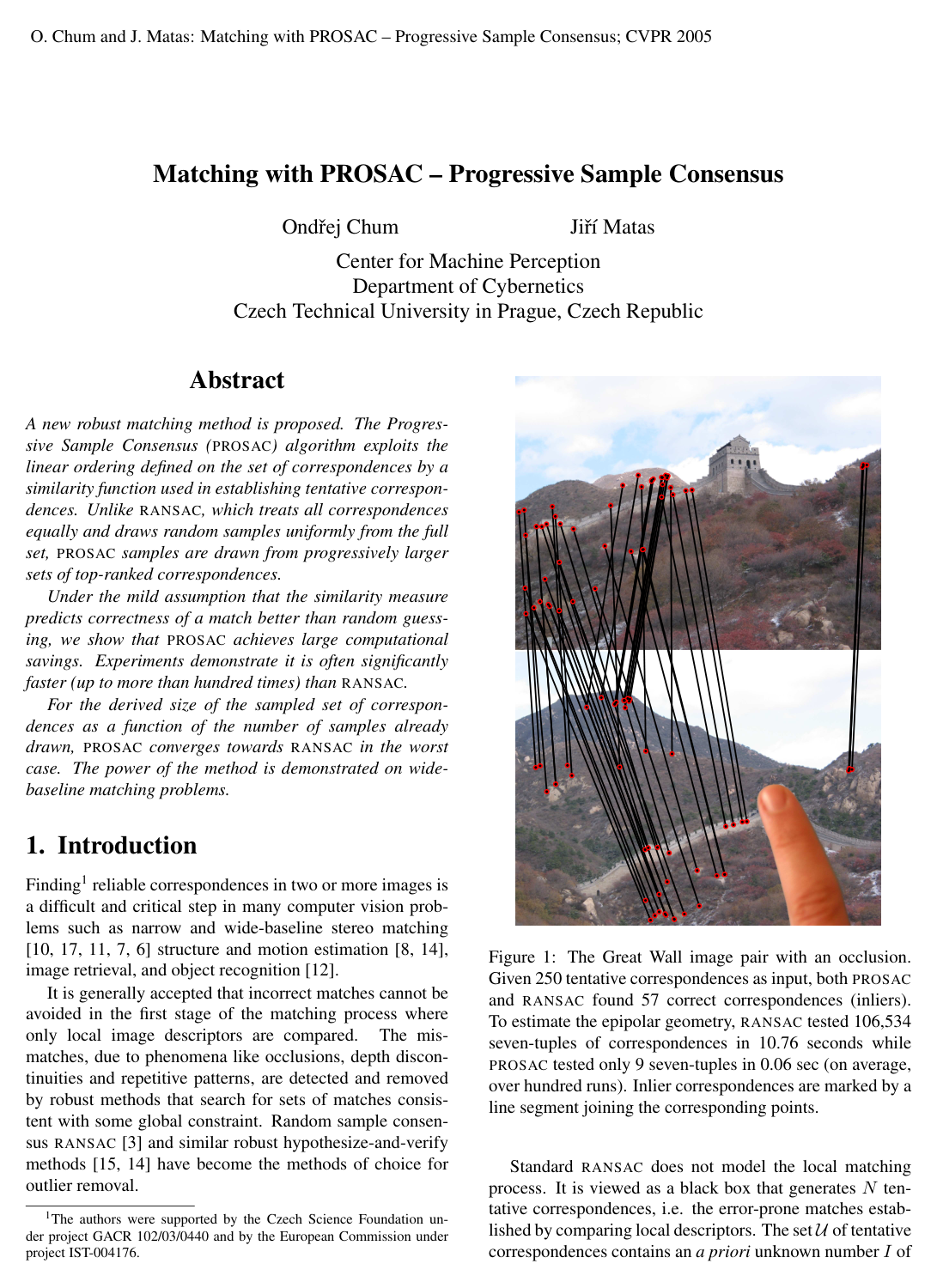
    Epipolar geometry estimation was evaluated on the Great Wall image pair with an occlusion, using N=250N = 250 tentative correspondences ranked by the Euclidean distance of the first 15 Discrete Cosine Transform (DCT) coefficients computed on affine-invariant parallelograms, with minimal sample size m=7m = 7.

    Both PROSAC and RANSAC detected the identical set of 57 inliers (inlier fraction ε=22.8%\varepsilon = 22.8\%). Standard RANSAC required an average of 106,534 sample evaluations and 10.76 seconds over 100 runs. PROSAC estimated the correct epipolar geometry after drawing an average of 9 samples in 0.06 seconds, yielding a speedup factor exceeding 170x in runtime and over 104×10^4\times in the number of tested hypotheses.

  7. Knowl 7 — Robustness to Low Inlier Fractions in the Plant Scene

    empirical result

    On the Plant scene—characterized by depth discontinuities, repetitive floor patterns, and self-similar foliage—tentative correspondences were established using Maximally Stable Extremal Regions (MSERs) with SIFT descriptor matching at a relaxed ratio threshold of 0.95, resulting in N=559N = 559 tentative matches with only I=51I = 51 inliers (inlier fraction ε=9.2%\varepsilon = 9.2\%).

    Under these low-inlier conditions, standard RANSAC failed practically because finding the 7-point epipolar geometry would require an average of 8.43×1078.43 \times 10^7 samples. PROSAC successfully isolated the inliers within the top-ranked correspondences and estimated the correct epipolar geometry in an average of 3,576 samples and 0.76 seconds over 100 runs.

  8. Knowl 8 — Performance on Two-Frame Motion Segmentation

    data/table

    Two-frame motion segmentation was evaluated on the non-rigid Mug dataset, where a mug moves independently against a static background. Matches were obtained using SIFT descriptors on MSER and affine-invariant regions. First, the dominant background epipolar geometry was estimated and inliers were removed; then, the secondary epipolar geometry of the foreground mug was estimated.

    Target Method Inliers (II) Samples (kk) Time [sec]
    Background PROSAC 617 1.0 0.33
    (N=783,ε=79%N = 783, \varepsilon = 79\%) RANSAC 617 15 1.10
    Mug (Foreground) PROSAC 51.6 18 0.12
    (N=166,ε=31%N = 166, \varepsilon = 31\%) RANSAC 52.3 10,551 0.96

    For the dominant background motion with high inlier density (79%), PROSAC converged in 1.0 sample on average versus 15 for RANSAC. For the lower inlier ratio of the foreground object (31%), PROSAC required 18 samples (0.12 s) compared to 10,551 samples (0.96 s) for RANSAC.

  9. Knowl 9 — Worst-Case Performance Under Random Correspondence Ordering

    data/table

    To evaluate PROSAC in the worst-case scenario where descriptor similarity provides no predictive sorting, the 250 tentative correspondences from the Great Wall scene (I=57I = 57 inliers) were randomly permuted across 100 independent runs.

    Method Mean kk Min kk Max kk Time [sec]
    RANSAC 106,534 97,702 126,069 10.76
    PROSAC (quality-sorted) 9 5 29 0.06
    PROSAC (random ordering) 61,263 1,465 110,727 6.28

    Even with completely random ordering, PROSAC required fewer samples on average (61,263) than RANSAC (106,534) because stochastic permutations naturally contain local sub-sequences with higher-than-average inlier concentrations that trigger early termination. The maximum sample count for randomly ordered PROSAC (110,727) was comparable to RANSAC, demonstrating that PROSAC converges to RANSAC performance in the worst case.

Coverage note — No substantial contributed material was omitted from the knowls.

References

  1. 1.M. Brown and D. Lowe. Recognising panoramas. In Proc. ICCV03, volume I, pages 1218–1225, October 2003.
  2. 2.O. Chum, J. Matas, and Š. Obdržálek. Enhancing RANSAC by generalized model optimization. In Proc. of the ACCV, volume 2, pages 812–817, January 2004.
  3. 3.M. Fischler and R. Bolles. Random sample consensus: A paradigm for model fitting with applications to image analysis and automated cartography. CACM, 24(6):381–395, June 1981.
  4. 4.R. Hartley and A. Zisserman. Multiple view geometry in computer vision. Cambridge University, Cambridge, 2nd edition, 2003.
  5. 5.D. Lowe. Distinctive image features from scale-invariant keypoints. International Journal of Computer Vision, 60(2):91–110, 2004.
  6. 6.J. Matas, O. Chum, M. Urban, and T. Pajdla. Robust wide-baseline stereo from maximally stable extremal regions. Image and Vision Computing, 22(10):761–767, Sep 2004.
  7. 7.K. Mikolajczyk and C. Schmid. An affine invariant interest point detector. In Proc. ECCV, volume 1, pages 128–142, 2002.
  8. 8.D. Nister. Preemptive RANSAC for live structure and motion estimation. In Proc. ICCV03, volume I, pages 199–206, October 2003.
  9. 9.Š. Obdržálek and J. Matas. Image retrieval using local compact DCT-based representation. In Proc. of DAGM’03, volume 1 of LNCS, pages 490–497. Springer-Verlag, 9 2003.
  10. 10.P. Pritchett and A. Zisserman. Wide baseline stereo matching. In Proc. ICCV, pages 754–760, 1998.
  11. 11.F. Schaffalitzky and A. Zisserman. Viewpoint invariant texture matching and wide baseline stereo. In Proc. 8th ICCV, Vancouver, Canada, July 2001.
  12. 12.H. Shao, T. Svoboda, T. Tuytelaars, and L. V. Gool. Hpat indexing for fast object/scene recognition based on local appearance. In computer lecture notes on Image and video retrieval, LNCS 2728, pages 71–80. Springers, July 2003.
  13. 13.J. Sivic and A. Zisserman. Video Google: A text retrieval approach to object matching in videos. In Proceedings of the International Conference on Computer Vision, pages 1470 – 1477, Oct. 2003.
  14. 14.B. Tordoff and D. Murray. Guided sampling and consensus for motion estimation. In Proc. 7th ECCV, volume 1, pages 82–96. Springer-Verlag, 2002.
  15. 15.P. H. S. Torr and A. Zisserman. MLESAC: A new robust estimator with application to estimating image geometry. CVIU, 78:138–156, 2000.
  16. 16.B. Triggs, P. McLauchlan, R. Hartley, and A. Fitzgibbon. A comprehensive survey of bundle adjustment in computer vision. In Proc. Vision Algorithms: Theory and Practice. International Workshop on Vision Algorithms, number 1883 in LNCS, pages 298–372. Springer Verlag, 1999.
  17. 17.T. Tuytelaars and L. Van Gool. Wide baseline stereo matching based on local, affinely invariant regions. In Proc. 11th BMVC, 2000.
  18. 18.Z. Zhang, R. Deriche, O. Faugeras, and Q.-T. Luong. A robust technique for matching two uncalibrated images through the recovery of the unknown epipolar geometry,. Artificial Intelligence, December 1995, 78:87–119, 1995.

Citation

MLA
Chum, O., and J. Matas. “Matching with PROSAC — Progressive Sample Consensus”. 2005 IEEE Computer Society Conference on Computer Vision and Pattern Recognition (CVPR'05), vol. 1, 2005, pp. 220–26, https://doi.org/10.1109/CVPR.2005.221.
APA
Chum, O., & Matas, J. (2005). Matching with PROSAC — Progressive Sample Consensus. 2005 IEEE Computer Society Conference on Computer Vision and Pattern Recognition (CVPR'05), 1, 220–226. https://doi.org/10.1109/CVPR.2005.221
Chicago
Chum, O., and J. Matas. 2005. “Matching with PROSAC — Progressive Sample Consensus”. 2005 IEEE Computer Society Conference on Computer Vision and Pattern Recognition (CVPR'05) 1: 220–26. https://doi.org/10.1109/CVPR.2005.221.
Harvard
Chum, O. and Matas, J. (2005) “Matching with PROSAC — Progressive Sample Consensus”, 2005 IEEE Computer Society Conference on Computer Vision and Pattern Recognition (CVPR'05). IEEE, pp. 220–226. Available at: https://doi.org/10.1109/CVPR.2005.221.
Vancouver
1. Chum O, Matas J (2005) Matching with PROSAC — Progressive Sample Consensus. In: 2005 IEEE Computer Society Conference on Computer Vision and Pattern Recognition (CVPR'05). IEEE, pp 220–226

BibTeX

@inproceedings{Chum, title={Matching with PROSAC — Progressive Sample Consensus}, volume={1}, url={http://dx.doi.org/10.1109/CVPR.2005.221}, DOI={10.1109/cvpr.2005.221}, booktitle={2005 IEEE Computer Society Conference on Computer Vision and Pattern Recognition (CVPR′05)}, publisher={IEEE}, author={Chum, O. and Matas, J.}, pages={220–226} }
Metadata:Crossref

Access the Paper

This paper is available from its original source. Click below to access the PDF.

Open PDF
License: IEEE