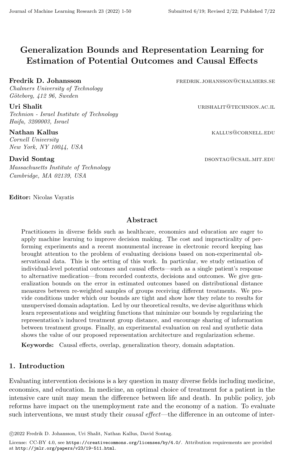
Generalization Bounds and Representation Learning for Estimation of Potential Outcomes and Causal Effects

Fredrik D. JohanssonUri ShalitNathan KallusDavid A. Sontag

article2022JMLR123 citations

Establishes theoretical generalization bounds for individual causal effect estimation from observational data and introduces representation learning algorithms that minimize distributional distance between treatment groups to achieve consistent potential outcome predictions.

Listen

Modern decision-makers in fields such as healthcare, economics, and public policy increasingly seek to use historical, observational records to guide personalized interventions. Conducting randomized controlled trials is often prohibitively expensive, unethical, or logistically impractical. However, drawing causal conclusions from observational data is fundamentally challenging due to confounding and treatment group imbalance, where individuals receiving different treatments systematically differ in baseline characteristics.

The article establishes theoretical performance bounds and develops practical machine learning algorithms to accurately estimate individual-level potential outcomes and conditional average treatment effects from observational data. It specifically demonstrates how combining sample re-weighting with representation learning bounds generalization error and enables consistent causal estimation even under imperfect treatment group overlap.

The authors analyze the problem through statistical learning theory and unsupervised domain adaptation. They derive finite-sample generalization bounds based on integral probability metrics, such as the Maximum Mean Discrepancy and Wasserstein distance, between treated and control groups in a learned, invertible representation space. Guided by this theory, the authors formulate neural network architectures—specifically Treatment-Agnostic Representation Networks (TARNet) and Counterfactual Regression (CFR) models—that jointly optimize outcome prediction, sample weights, and group distributional balance. The methods are evaluated across synthetic, semi-synthetic (IHDP, with 747 subjects and 1,000 outcome realizations), and real-world benchmark datasets (the Jobs dataset, comprising 3,212 subjects).

The evaluation yields several key findings. First, neural network architectures with shared representations significantly outperform standard baselines, with CFR achieving out-of-sample mean squared errors of 0.76 to 0.78 on the IHDP benchmark compared to 2.3 for Bayesian Additive Regression Trees and 3.8 for Causal Forests. Second, regularizing the distributional distance between treatment groups consistently reduces counterfactual prediction error, though excessive penalties harm performance if representations lose predictive detail. Third, jointly learning sample weights alongside representations mitigates sensitivity to heavy regularization and provides an effective bias-variance trade-off. Finally, on the Jobs benchmark, nonlinear representation models achieve the lowest out-of-sample policy risk (0.21 compared to 0.23–0.28 for linear and random forest baselines), although handcrafted features in lower dimensions reduce the performance gap between simple and complex models.

These findings demonstrate that organizations can reliably use observational data to guide high-stakes, personalized interventions by properly penalizing covariate imbalance in learned representations. The framework bridges the gap between traditional propensity-based sample weighting and flexible deep learning, offering formal guarantees even when standard overlap assumptions are partially violated. This reduces the risk of making costly policy or clinical errors caused by observational selection bias.

Organizations implementing machine learning for causal decision-making should adopt shared-representation architectures with distributional balancing rather than fitting completely separate regression models for each treatment. Practitioners should also consider jointly learning sample weights to prevent extreme variance in small samples or regions of poor overlap. Before broad deployment in complex settings such as electronic health records, teams should conduct pilot studies and sensitivity analyses, as the current empirical validation relies on relatively small, stylized benchmarks.

The theoretical guarantees assume that all confounding variables are measured (ignorability) and that representations remain invertible. In real-world applications where unobserved confounding exists or the number of treatment options is large, readers should exercise appropriate caution, as observational data alone cannot fully verify these underlying causal assumptions.

Chalmers University of Technology Cornell University Massachusetts Institute of Technology Technion – Israel Institute of Technology representation learning treatment effect estimation potential outcomes generalization bounds

arXiv: 2001.07426

Paper: Estimating individual treatment effect: generalization bounds and algorithms, Uri Shalit et al. (2016). This seminal work establishes the foundational error bounds and counterfactual regression representation learning framework that the source directly generalizes and tightens.
Paper: A theory of learning from different domains, Shai Ben-David et al. (2010). It provides the foundational domain adaptation generalization theory and distribution discrepancy bounds that the source adapts to the potential outcomes estimation setting.
Paper: Correcting Sample Selection Bias by Unlabeled Data, Jiayuan Huang et al. (2006). It introduces distribution matching via sample reweighting in feature spaces, a core technique utilized by the source to balance observational treatment groups.
Paper: Domain Generalization via Invariant Feature Representation, Krikamol Muandet et al. (2013). It establishes domain-invariant component analysis and theoretical bounds for invariant representations that motivate the source's representation learning objectives.
Paper: Estimation and Inference of Heterogeneous Treatment Effects using Random Forests, Stefan Wager et al. (2018). It establishes essential non-parametric methodology and asymptotic properties for estimating heterogeneous treatment effects from observational data.
Paper: Recursive partitioning for heterogeneous causal effects, Susan Athey et al. (2015). It introduces fundamental principles of recursive partitioning and honest sample-splitting for identifying heterogeneous causal effects.
Paper: Counterfactual Risk Minimization: Learning from Logged Bandit Feedback, Adith Swaminathan et al. (2015). It introduces counterfactual risk minimization principles that combine importance-weighted empirical loss with variance regularization from logged observational feedback.

Paper: Nonparametric Identifiability of Causal Representations from Unknown Interventions, Julius von Kügelgen et al. (2023). It extends causal representation learning to the nonparametric identifiability of latent causal variables and graphs under unknown interventions across multiple environments.
Paper: Change is Hard: A Closer Look at Subpopulation Shift, Yuzhe Yang et al. (2023). It evaluates and analyzes the practical generalization failures and representation learning dynamics of algorithms across structured subpopulation and distribution shifts.
Paper: Linear Causal Disentanglement via Interventions, Chandler Squires et al. (2023). It provides identifiability guarantees for latent causal disentanglement and representations learned from observational and interventional data.
Paper: Identifying Weight-Variant Latent Causal Models, Yuhang Liu et al. (2026). It builds upon causal representation principles by establishing identifiability conditions for weight-variant latent causal models from observational distributions.

Cover for Generalization Bounds and Representation Learning for Estimation of Potential Outcomes and Causal Effects

Abstract

Practitioners in diverse fields such as healthcare, economics and education are eager to apply machine learning to improve decision making. The cost and impracticality of performing experiments and a recent monumental increase in electronic record keeping has brought attention to the problem of evaluating decisions based on non-experimental observational data. This is the setting of this work. In particular, we study estimation of individual-level potential outcomes and causal effects—such as a single patient's response to alternative medication—from recorded contexts, decisions and outcomes. We give generalization bounds on the error in estimated outcomes based on distributional distance measures between re-weighted samples of groups receiving different treatments. We provide conditions under which our bounds are tight and show how they relate to results for unsupervised domain adaptation. Led by our theoretical results, we devise algorithms which learn representations and weighting functions that minimize our bounds by regularizing the representation's induced treatment group distance, and encourage sharing of information between treatment groups. Finally, an experimental evaluation on real and synthetic data shows the value of our proposed representation architecture and regularization scheme.

Topics

representation learning

Keywords

treatment effect estimation potential outcomes generalization bounds representation learning causal inference selection bias domain adaptation propensity weighting methods neural network estimators Bayesian additive regression trees

1. Introduction
1.1 Notation and Terminology
2. Potential Outcomes and Effects of Interventions
2.1 Identifying Assumptions
3. Related Work
4. Generalization Bounds for Estimating Potential Outcomes and CATE
4.1 Risk for Hypotheses of Potential Outcomes and CATE
4.2 Importance-weighting Hypotheses & Propensity Scores
4.3 Bounds on the Risk of a Re-weighted Estimator
4.4 Bounds Based on Finite Samples
5. Generalization Bounds for Representation Learning
5.1 Relation to Unsupervised Domain Adaptation
6. Estimation
6.1 A First Learning Objective and Asymptotic Consistency
6.2 Practical Representation Learning and Learning Shared Representations
6.3 Implementing Regularization of Distributional Distance
7. Experiments
7.1 Experimental Setup & Baselines
7.1.1 Evaluation Criteria & Hyperparameter Selection
7.2 Synthesized Outcome: IHDP
7.3 Partially Randomized Study: National Supported Work Program
8. Discussion
Acknowledgments
Appendix A. Proof of Theorem 3
Appendix B. Experiment Details
Appendix C. Architecture for Joint Learning of Sample Weights
Appendix D. Minimization of Approximate Wasserstein Distances
References

Knowls

Knowl 1 — Generalization Bound for Counterfactual Risk under Invertible Representations and Sample Weighting
theoretical result
Let context covariates be denoted $X \in \mathcal{X} \subseteq \mathbb{R}^d$ , binary treatment by $T \in \{0, 1\}$ , and potential outcomes by $Y(0), Y(1) \in \mathcal{Y} \subset [-\omega, \omega]$ for finite $\omega > 0$ . Let $p(X, T, Y)$ be the observational population distribution with conditional treatment densities $p_t(x) = p(X = x \mid T = t)$ and marginal treatment probabilities $\pi_t = p(T = t)$ .

Assume strong ignorability holds with respect to $X$ , namely $(Y(0), Y(1)) \perp T \mid X$ . Let $\Phi: \mathcal{X} \to \mathcal{Z} \subset \mathbb{R}^v$ be a twice-differentiable, invertible representation function with inverse $\Psi = \Phi^{-1}: \mathcal{Z} \to \mathcal{X}$ and Jacobian determinant $J_\Psi(z) = \det(\nabla_z \Psi(z))$ . Let $A_\Phi > 0$ be a finite constant such that $|J_\Psi(z)| \le A_\Phi$ for all $z \in \mathcal{Z}$ .

Let $h_t: \mathcal{Z} \to \mathcal{Y}$ be a hypothesis operating on representations, defining the composite hypothesis $f_t(x) = h_t(\Phi(x)) \in \mathcal{H}$ . Let $L(y, y') = (y - y')^2$ denote the squared loss, and define the conditional representation loss $\ell_{\Phi, h_t}(z) := \mathbb{E}_{Y(t) \mid X}[L(h_t(z), Y(t)) \mid X = \Psi(z)]$ . Let $B_\Phi > 0$ be a constant such that with $C_\Phi := A_\Phi B_\Phi$ , the scaled loss satisfies $\ell_{\Phi, h_t} / C_\Phi \in \mathcal{L}$ , where $\mathcal{L}$ is a reproducing kernel Hilbert space (RKHS) associated with a universal kernel $k$ satisfying $\sup_{x \in \mathcal{X}} k(x, x) < \infty$ .

Let $w_t: \mathcal{Z} \to \mathbb{R}_+$ be any non-negative sample weighting function satisfying $\mathbb{E}_{Z \sim p_{\Phi, t}}[w_t(Z)] = 1$ , where $p_{\Phi, t}$ is the density of $\Phi(X)$ conditional on $T = t$ , and let $\hat{p}_{\Phi, t}^{w_t}$ denote the weighted empirical representation distribution over an i.i.d. sample of size $n$ with $n_t = \sum_{i=1}^n \mathbf{1}[t_i = t]$ .

Then, with probability at least $1 - 2\delta$ over the sample draw, the counterfactual risk $R_{1-t}(f_t) = \mathbb{E}_{X \mid T = 1-t}[(f_t(X) - Y(t))^2]$ is bounded by:

$R_{1-t}(f_t) \le \hat{R}_t^{w_t}(f_t) + C_\Phi \cdot \text{IPM}_\mathcal{L}\left(\hat{p}_{\Phi, 1-t}, \hat{p}_{\Phi, t}^{w_t}\right) + V_{p_t}(w_t, \ell_{f_t}) \frac{C_{n_t, \delta}^\mathcal{H}}{n_t^{3/8}} + D_{n_0, n_1, \delta}^{\Phi, \mathcal{L}} \left(\frac{1}{\sqrt{n_0}} + \frac{1}{\sqrt{n_1}}\right) + \sigma_{Y(t)}^2$

where:
- $\hat{R}_t^{w_t}(f_t) = \frac{1}{n_t} \sum_{i: t_i = t} w_t(\Phi(x_i)) (y_i - f_t(x_i))^2$ is the weighted empirical factual risk.
- $\text{IPM}_\mathcal{L}(p, q) = \sup_{\ell \in \mathcal{L}} |\mathbb{E}_p[\ell] - \mathbb{E}_q[\ell]|$ is the Integral Probability Metric w.r.t. $\mathcal{L}$ .
- $C_{n_t, \delta}^\mathcal{H} = 2^{5/4} \left(d \log \frac{2 n_t e}{d} + \log \frac{4}{\delta}\right)^{3/8}$ , where $d = \text{Pdim}(\{\ell_h : h \in \mathcal{H}\})$ is the pseudo-dimension of the loss-composed hypothesis class.
- $D_{n_0, n_1, \delta}^{\Phi, \mathcal{L}} = \sqrt{18 \nu^2 C \log(4/\delta)}$ with $\nu = \sup_{z \in \mathcal{Z}, \ell \in \mathcal{L}} \ell(z)$ and $C = \sup_{z} k(z, z)$ .
- $V_{p_t}(w_t, \ell_{f_t}) = \max\left(\sqrt{\mathbb{E}_{p_t}[w_t^2(X) \ell_{f_t}^2(X)]}, \sqrt{\mathbb{E}_{\hat{p}_t}[w_t^2(X) \ell_{f_t}^2(X)]}\right)$ .
- $\sigma_{Y(t)}^2 = \mathbb{E}_{X, Y(t)}[(Y(t) - \mathbb{E}[Y(t) \mid X])^2]$ is the conditional variance of the potential outcome.
This bound is valid both with and without complete treatment group overlap in covariate space $\mathcal{X}$ .
Knowl 2 — Asymptotic Consistency of Joint Optimization of Representations, Hypotheses, and Balancing Weights
theoretical result
Let hypothesis class $\mathcal{H}$ be a reproducing kernel Hilbert space (RKHS) induced by a bounded kernel $k$ such that for any hypothesis $h_t \in \mathcal{G}$ and representation $\Phi \in \mathcal{E}$ , the composition $h_t \circ \Phi \in \mathcal{H}$ . Let the integral probability metric (IPM) function space $\mathcal{L}$ be an RKHS with bounded kernel $k_\mathcal{L}$ .

Assume weak overlap holds between treatment groups: for each $t \in \{0, 1\}$ ,

$\mathbb{E}_X\left[\left(\frac{p_t(X)}{p_{1-t}(X)}\right)^2\right] < \infty$

where $p_t(X) = p(X \mid T = t)$ . For a sample size $n$ with $n_t = \sum_{i=1}^n \mathbf{1}[t_i = t]$ , let $\mathcal{O}_t(h_t, \Phi, w^t; \beta)$ be the regularized weighted factual objective defined with hyperparameters $\beta = (\alpha, \lambda_h, \lambda_w)$ :

$\mathcal{O}_t(h_t, \Phi, w^t; \beta) = \sum_{i: t_i = t} \frac{\tilde{w}_i^t}{n_t} L(h_t(\Phi(x_i)), y_i) + \frac{\lambda_h}{\sqrt{n_t}} \mathcal{R}(h_t) + \alpha \pi_{1-t} \text{IPM}_\mathcal{L}\left(\hat{p}_{\Phi, t}^{w^t}, \hat{p}_{\Phi, 1-t}\right) + \frac{\lambda_w}{n_t} \|w^t\|_2^2$

subject to $\sum_{i: t_i = t} w_i^t = n_t$ , where $\tilde{w}_i^t = \pi_t + \pi_{1-t} w_i^t$ , $\pi_t = p(T = t)$ , and $\mathcal{R}(h_t)$ is a complexity regularizer on $h_t$ .

Then the minimum empirical objective satisfies:

$\min_{h_t, \Phi, w^t} \mathcal{O}_t(h_t, \Phi, w^t; \beta) \le \min_{f_t \in \mathcal{H}} R(f_t) + O_p\left(\frac{1}{\sqrt{n_0}} + \frac{1}{\sqrt{n_1}}\right)$

where $R(f_t) = \mathbb{E}_{X, Y(t)}[L(f_t(X), Y(t))]$ is the true marginal population risk and $O_p$ denotes stochastic boundedness. Furthermore, for sufficiently large $\alpha$ and $\lambda_w$ , the minimizer $\hat{f}_n^t = \hat{h}_t \circ \hat{\Phi}$ satisfies:

$R(\hat{f}_n^t) \le \min_{f_t \in \mathcal{H}} R(f_t) + O_p\left(n_0^{-3/8} + n_1^{-3/8}\right)$

proving that the empirical minimizers converge to the representation and hypothesis that minimize the counterfactual risk in the large-sample limit.
Knowl 3 — Counterfactual Regression (CFR) and Re-weighted CFR (RCFR) Estimator Architectures and Objectives
model/method
The Counterfactual Regression (CFR) and Re-weighted CFR (RCFR) models estimate individual potential outcomes and conditional average treatment effects by combining deep shared representations with distributional imbalance regularization and sample re-weighting.

The neural architecture consists of:
1. A shared representation sub-network $\Phi: \mathcal{X} \to \mathcal{Z}$ parameterized by feed-forward layers that map context features $x \in \mathbb{R}^d$ to an embedding $z \in \mathbb{R}^v$ .
2. Two treatment-specific head sub-networks $h_0, h_1: \mathcal{Z} \to \mathcal{Y}$ , where $h_0$ predicts potential outcome under control $Y(0)$ and $h_1$ predicts potential outcome under treatment $Y(1)$ .
3. In RCFR, an auxiliary weighting network $w: \mathcal{X} \times \{0, 1\} \to \mathbb{R}_+$ predicting sample weights $w_i = w(x_i, t_i)$ subject to $\sum_{i: t_i = t} w_i = n_t$ .
The unregularized baseline, Treatment-Agnostic Representation Network (TARNet), minimizes factual prediction error across both treatment groups:

$\mathcal{O}_{\text{TARNet}}(h, \Phi) = \frac{1}{n} \sum_{i=1}^n L(h(\Phi(x_i), t_i), y_i) + \frac{\lambda_h}{\sqrt{n}} \mathcal{R}(h)$

The CFR estimator penalizes the distributional distance between treated and control groups in representation space:

$\mathcal{O}_{\text{CFR}}(h, \Phi) = \frac{1}{n} \sum_{i=1}^n L(h(\Phi(x_i), t_i), y_i) + \alpha \cdot \text{IPM}_\mathcal{L}(\hat{p}_{\Phi, 0}, \hat{p}_{\Phi, 1}) + \frac{\lambda_h}{\sqrt{n}} \mathcal{R}(h)$

The RCFR estimator incorporates learned sample weights $w$ to trade off representation constraint with variance control:

$\mathcal{O}_{\text{RCFR}}(h, \Phi, w) = \sum_{i=1}^n \frac{w_i}{n} L(h(\Phi(x_i), t_i), y_i) + \alpha \cdot \text{IPM}_\mathcal{L}\left(\hat{p}_{\Phi, 0}^{w_0}, \hat{p}_{\Phi, 1}^{w_1}\right) + \frac{\mathcal{R}(h)}{\lambda_h^{-1} \sqrt{n}} + \frac{\|w\|_2^2}{\lambda_w^{-1} n}$

where $\text{IPM}_\mathcal{L}$ is instantiated either as Maximum Mean Discrepancy (MMD) or Wasserstein distance.
Knowl 4 — CATE Generalization Error Bound via Potential Outcome Prediction Risks
theoretical result
Let $\mu_t(x) = \mathbb{E}[Y(t) \mid X = x]$ denote the conditional expectation of potential outcome $Y(t)$ for $t \in \{0, 1\}$ , and let $\tau(x) = \mu_1(x) - \mu_0(x)$ denote the Conditional Average Treatment Effect (CATE). Let $f_0, f_1 \in \mathcal{H}$ be hypotheses predicting $\mu_0, \mu_1$ , and define the estimated CATE function by $\hat{\tau}(x) = f_1(x) - f_0(x)$ .

Let the marginal population risk under squared loss $L(y, y') = (y - y')^2$ be $R(\hat{\tau}) = \mathbb{E}_X[(\tau(X) - \hat{\tau}(X))^2]$ and $R(f_t) = \mathbb{E}_{X, Y(t)}[(Y(t) - f_t(X))^2]$ . Then:

$R(\hat{\tau}) \le 2 \left(R(f_0) + R(f_1)\right) - 4 \sigma_Y^2$

where $\sigma_Y^2 = \max\left(\mathbb{E}_{X, Y(0)}[(Y(0) - \mu_0(X))^2], \mathbb{E}_{X, Y(1)}[(Y(1) - \mu_1(X))^2]\right)$ is the maximal residual outcome variance.

Furthermore, for an empirical dataset of size $n = n_0 + n_1$ with $n_{\min} = \min(n_0, n_1)$ , let $\hat{R}_p^{\tilde{w}}(f) = \frac{1}{n} \sum_{i=1}^n \tilde{w}(x_i, t_i) L(f(x_i, t_i), y_i)$ be the weighted empirical factual risk where $\tilde{w}(x, t) = w_t(x) / \pi_t$ . There exists a term $K_{\mathcal{L}, \mathcal{H}, w, \delta, n_0, n_1}$ with at most logarithmic dependence on $n_0, n_1$ such that with probability at least $1 - 2\delta$ :

$\frac{R(\hat{\tau})}{2} \le \hat{R}_p^{\tilde{w}}(f) + B \left[\pi_0 \text{IPM}_\mathcal{L}(\hat{p}_0, \hat{p}_1^{w_1}) + \pi_1 \text{IPM}_\mathcal{L}(\hat{p}_1, \hat{p}_0^{w_0})\right] + \frac{K_{\mathcal{L}, \mathcal{H}, w, \delta, n_0, n_1}}{n_{\min}^{3/8}} + 2\sigma_Y^2$

where $B > 0$ scales the loss space $\mathcal{L}$ , and $\pi_t = p(T = t)$ .
Knowl 5 — Counterfactual and Marginal Risk Bounds via Integral Probability Metrics
theoretical result
Let context $X \sim p(X)$ and treatment conditional distributions be $p_t(X) = p(X \mid T = t)$ with $\pi_t = p(T = t)$ for $t \in \{0, 1\}$ . The marginal population risk of a hypothesis $f_t$ w.r.t. potential outcome $Y(t)$ decomposes into an observable factual risk $R_t(f_t)$ and an unobserved counterfactual risk $R_{1-t}(f_t)$ :

$R(f_t) = \pi_t R_t(f_t) + (1 - \pi_t) R_{1-t}(f_t)$

Let $\ell_{f_t}(x) = \mathbb{E}_{Y(t) \mid X}[L(f_t(x), Y(t)) \mid X = x]$ belong to a normed family of pointwise loss functions $\mathcal{L}$ such that $\ell_{f_t} / \|\ell_{f_t}\|_\mathcal{L} \in \mathcal{L}$ . For any non-negative sample weighting function $w: \mathcal{X} \to \mathbb{R}_+$ satisfying $\mathbb{E}_{X \mid T = t}[w(X)] = 1$ , and re-weighted density $p_t^w(x) = p_t(x)w(x)$ :

$R_{1-t}(f_t) - R_t^w(f_t) \le \|\ell_{f_t}\|_\mathcal{L} \cdot \text{IPM}_\mathcal{L}(p_{1-t}, p_t^w)$

where $\text{IPM}_\mathcal{L}(p, q) = \sup_{\ell \in \mathcal{L}} |\mathbb{E}_p[\ell(X)] - \mathbb{E}_q[\ell(X)]|$ .

Defining combined weights $\tilde{w}(x) := \pi_t + (1 - \pi_t)w(x)$ , the total population risk is bounded by:

$R(f_t) \le R_t^{\tilde{w}}(f_t) + (1 - \pi_t) \|\ell_{f_t}\|_\mathcal{L} \cdot \text{IPM}_\mathcal{L}(p_{1-t}, p_t^w)$

If the treatment group overlap condition holds, the importance weighting function $w^*(x) = p_{1-t}(x) / p_t(x)$ yields $\text{IPM}_\mathcal{L}(p_{1-t}, p_t^{w^*}) = 0$ , making the counterfactual bound exact. The bound holds without overlap as long as $w(x)$ is defined on the support of $p_t(x)$ .
Knowl 6 — Stochastic Gradient Computation for Wasserstein Regularization via Sinkhorn Iteration
algorithm
The Wasserstein distance between empirical distributions in representation space is approximated using entropic regularization and differentiated via the Sinkhorn fixed-point iteration algorithm.
Input: Factual dataset samples $(x_1, t_1, y_1), \dots, (x_n, t_n, y_n)$ , representation network $\Phi_W$ with parameters $W$ , mini-batch size $m$ , entropic regularization scale $\lambda$ .
Output: Parameter gradient vector $g_1 = \nabla_W \text{Wass}(\hat{p}_{\Phi, 0}, \hat{p}_{\Phi, 1})$ .
Sample a mini-batch of $m$ control units $(x_{i_1}, 0, y_{i_1}), \dots, (x_{i_m}, 0, y_{i_m})$ and $m$ treated units $(x_{i_{m+1}}, 1, y_{i_{m+1}}), \dots, (x_{i_{2m}}, 1, y_{i_{2m}})$
Compute pairwise Euclidean distance matrix $M(\Phi_W) \in \mathbb{R}^{m \times m}$ :
$M_{kl}(\Phi_W) = \|\Phi_W(x_{i_k}) - \Phi_W(x_{i_{m+l}})\|_2$
Compute kernel matrix $K \in \mathbb{R}^{m \times m}$ where $K_{kl} = \exp(-\lambda M_{kl}(\Phi_W))$
Initialize scaling vector $u_0 = \mathbf{1}_m / m$
for fixed-point step $t = 0, 1, \dots, T-1$ do
$u_{t+1} = \frac{1}{m} \cdot \frac{1}{K (\frac{1}{m} \cdot \frac{1}{K^\top u_t})}$
end for
Compute approximate optimal transport coupling matrix $T^* = \text{diag}(u_T) K \text{diag}\left(\frac{1}{m K^\top u_T}\right)$
Compute stochastic gradient $g_1 = \nabla_W \langle T^*, M(\Phi_W) \rangle$
return $g_1$
The fixed-point update is unrolled as a recurrent neural network graph, allowing backpropagation of gradients with respect to network weights $W$ using automatic differentiation frameworks.
Knowl 7 — Potential Outcomes, CATE, and Risk Minimization under Confounding
definition
In the Neyman-Rubin potential outcome framework for observational causal inference:
- Context: $X \in \mathcal{X} \subseteq \mathbb{R}^d$ denotes observed baseline covariates.
- Treatment: $T \in \{0, 1\}$ is a binary treatment assignment.
- Observed Outcome: $Y = Y(T) \in \mathcal{Y} \subseteq \mathbb{R}$ is the factual observed response.
- Potential Outcomes: $Y(0), Y(1) \in \mathcal{Y}$ represent outcomes that would be observed under control and treatment, respectively, obeying the Stable Unit Treatment Value Assumption (SUTVA: $Y = T Y(1) + (1-T)Y(0)$ ).
The primary estimands are:
1. Expected potential outcomes: $\mu_t(x) := \mathbb{E}[Y(t) \mid X = x]$ for $t \in \{0, 1\}$ .
2. Conditional average treatment effect (CATE): $\tau(x) := \mathbb{E}[Y(1) - Y(0) \mid X = x] = \mu_1(x) - \mu_0(x)$ .
Under point loss $L: \mathcal{Y} \times \mathcal{Y} \to \mathbb{R}_+$ , the expected pointwise loss is $\ell_{f_t}(x) = \mathbb{E}[L(Y(t), f_t(x)) \mid X = x]$ .
- Marginal population risk: $R(f_t) := \mathbb{E}_{X \sim p(X)}[\ell_{f_t}(X)]$ .
- Factual risk: $R_t(f_t) := \mathbb{E}_{X \mid T = t}[\ell_{f_t}(X)]$ .
- Counterfactual risk: $R_{1-t}(f_t) := \mathbb{E}_{X \mid T = 1-t}[\ell_{f_t}(X)]$ .
- CATE risk: $R(\hat{\tau}) := \mathbb{E}_{X \sim p(X)}[L(\tau(X), \hat{\tau}(X))]$ .
Identification requires:
- Ignorability: $(Y(0), Y(1)) \perp T \mid X$ .
- Overlap: $\forall x \in \mathcal{X}, t \in \{0, 1\}: p(T = t \mid X = x) > 0$ .

Knowl 8 — Comparative Evaluation of CATE Estimation on the IHDP Benchmark

data/table

The Infant Health and Development Program (IHDP) benchmark comprises 747 units (139 treated, 608 control) with 25 baseline covariates. Selection bias is induced by removing all treated children with non-white mothers, creating overlap deficiency in correlated features. The outcome is generated via a semi-synthetic response surface (setting 'A' in NPCI, response surface 'B' in Hill 2011) with an exponential-linear treated outcome and linear control outcome, yielding a non-linear CATE function across 1000 randomized draws.

Evaluation is measured using Mean Squared Error (MSE) in CATE estimation and MSE in Average Treatment Effect (ATE) estimation, reported with standard errors over 1000 realizations:

	Within sample		Out of sample
Model	MSE CATE	MSE ATE	MSE CATE	MSE ATE
OLS-S	$5.8 \pm 0.3$	$0.73 \pm 0.04$	$5.8 \pm 0.3$	$0.94 \pm 0.06$
OLS-T	$2.4 \pm 0.1$	$0.14 \pm 0.01$	$2.5 \pm 0.1$	$0.31 \pm 0.02$
BLR	$5.8 \pm 0.3$	$0.72 \pm 0.04$	$5.8 \pm 0.3$	$0.93 \pm 0.05$
k-NN	$2.1 \pm 0.1$	$0.14 \pm 0.01$	$4.1 \pm 0.2$	$0.79 \pm 0.05$
TMLE	$5.0 \pm 0.2$	$0.30 \pm 0.01$	–	–
BART	$2.1 \pm 0.1$	$0.23 \pm 0.01$	$2.3 \pm 0.1$	$0.34 \pm 0.02$
R.For.	$4.2 \pm 0.2$	$0.73 \pm 0.05$	$6.6 \pm 0.3$	$0.96 \pm 0.06$
C.For.	$3.8 \pm 0.2$	$0.18 \pm 0.01$	$3.8 \pm 0.2$	$0.40 \pm 0.03$
BNN	$2.2 \pm 0.1$	$0.37 \pm 0.03$	$2.1 \pm 0.1$	$0.42 \pm 0.03$
TARNet	$0.88 \pm 0.02$	$0.26 \pm 0.01$	$0.95 \pm 0.02$	$0.28 \pm 0.01$
CFR $_{\text{MMD}}$	$0.73 \pm 0.01$	$0.30 \pm 0.01$	$0.78 \pm 0.02$	$0.31 \pm 0.01$
CFR $_{\text{Wass}}$	$0.71 \pm 0.02$	$0.25 \pm 0.01$	$0.76 \pm 0.02$	$0.27 \pm 0.01$

Shared representation networks (TARNet, CFR) substantially outperform single-model (S-learner) and tree-based baselines. Regularizing representation distance (CFR $_{\text{MMD}}$ and CFR $_{\text{Wass}}$ ) further reduces out-of-sample CATE error relative to TARNet ( $0.76-0.78$ vs $0.95$ ). Imbalance penalty tuning shows that optimal error is achieved around $\alpha \approx 1$ ; for $\alpha > 2$ , performance degrades unless joint sample weight optimization (RCFR) is applied.

Knowl 9 — Policy Risk and ATT Estimation on the Partially Randomized Jobs Benchmark

data/table

The Jobs dataset evaluates causal effect estimation using a combined experimental and observational design based on the National Supported Work (NSW) study and the PSID control group. The dataset contains 297 treated units (all from NSW), 425 experimental control units, and 2490 non-experimental observational controls (3212 units total, 482 unemployed). The experimental and observational cohorts are separated with 96% accuracy by a linear classifier, creating severe lack of overlap.

Evaluation is performed over 10 train/validation/test splits (56/24/20 ratio). Metrics are policy risk $\hat{R}_{\text{Pol}}(\pi)$ (expected unemployment rate under the policy $\pi_f(x) = \mathbf{1}[f(x, 1) - f(x, 0) > 0]$ , evaluated on the randomized sub-population via propensity rejection sampling) and Mean Squared Error on the Average Treatment Effect on the Treated (MSE ATT):

	Within sample		Out of sample
Model	$\hat{R}_{\text{Pol}}$	MSE ATT	$\hat{R}_{\text{Pol}}$	MSE ATT
LR-S	$0.22 \pm 0.00$	$0.01 \pm 0.00$	$0.23 \pm 0.02$	$0.08 \pm 0.04$
LR-T	$0.21 \pm 0.00$	$0.01 \pm 0.01$	$0.24 \pm 0.01$	$0.08 \pm 0.03$
BLR	$0.22 \pm 0.01$	$0.01 \pm 0.01$	$0.25 \pm 0.02$	$0.08 \pm 0.03$
k-NN	$0.02 \pm 0.00$	$0.21 \pm 0.01$	$0.26 \pm 0.02$	$0.13 \pm 0.05$
TMLE	$0.22 \pm 0.00$	$0.02 \pm 0.01$	–	–
BART	$0.23 \pm 0.00$	$0.02 \pm 0.00$	$0.25 \pm 0.02$	$0.08 \pm 0.03$
R.For.	$0.23 \pm 0.01$	$0.03 \pm 0.01$	$0.28 \pm 0.02$	$0.09 \pm 0.04$
C.For.	$0.19 \pm 0.00$	$0.03 \pm 0.01$	$0.20 \pm 0.02$	$0.07 \pm 0.03$
BNN	$0.20 \pm 0.01$	$0.04 \pm 0.01$	$0.24 \pm 0.02$	$0.09 \pm 0.04$
TARNet	$0.17 \pm 0.01$	$0.05 \pm 0.02$	$0.21 \pm 0.01$	$0.11 \pm 0.04$
CFR $_{\text{MMD}}$	$0.18 \pm 0.00$	$0.04 \pm 0.01$	$0.21 \pm 0.01$	$0.08 \pm 0.03$
CFR $_{\text{Wass}}$	$0.17 \pm 0.01$	$0.04 \pm 0.01$	$0.21 \pm 0.01$	$0.09 \pm 0.03$

TARNet and CFR achieve the lowest policy risk ( $0.21$ out-of-sample). On this benchmark, linear models perform competitively for ATT estimation because features were handcrafted for linear confounding adjustment, resulting in smaller relative gains for non-linear representation balancing compared to IHDP.

Knowl 10 — Role of Invertibility, Jacobian Scaling, and Confounder Disentanglement in Representation Bounds
limitation
The theoretical validity and tightness of representation-based causal generalization bounds depend on specific properties of the representation $\Phi$ :
1. Invertibility and Ignorability: If $\Phi$ is non-invertible, information in $X$ that is predictive of $Y$ may be discarded to artificially reduce the distributional distance $\text{IPM}_\mathcal{L}(p_{\Phi, 0}, p_{\Phi, 1})$ . Discarding predictive confounders destroys conditional ignorability in representation space ( $Y(t) \not\perp T \mid \Phi(X)$ ), rendering counterfactual predictions biased.
2. Scale Distortion and Jacobian Factor $C_\Phi$ : If $\Phi$ simply shrinks the input space (e.g., $\Phi(x) = x / a$ for $a > 1$ ), IPM distances decrease trivially. The bound compensates through the constant $C_\Phi = A_\Phi B_\Phi \ge |\det(\nabla_z \Phi^{-1}(z))| B_\Phi$ , which scales inversely with volume compression. Fixing the regularization weight $\alpha$ independently of $\Phi$ during training may cause over- or under-penalization.
3. Instrumental and Non-Confounding Variables: If covariates $X$ contain instrumental variables (predictive of $T$ but not directly causal of $Y$ ), they increase the IPM distance without improving outcome prediction. While learning $\Phi$ can suppress such variables, unconstrained distance penalties on non-invertible embeddings risk removing genuine confounders.
4. Overlap Verification: When overlap is absent, the assumption that the true loss $\ell_{\Phi, h_t} / C_\Phi \in \mathcal{L}$ cannot be verified from observational data alone.

Coverage note — None was omitted; all key theoretical bounds (Theorems 1-3, Lemmas 1-3, Lemma 6, Corollary 1-2), estimator models (TARNet, CFR, RCFR), Sinkhorn optimization algorithm, empirical datasets (IHDP and Jobs tables), and analysis of limitations are represented.

References

1.Alberto Abadie and Guido W Imbens. Matching on the estimated propensity score. Econometrica, 84(2):781–807, 2016.
2.Jason Abrevaya, Yu-Chin Hsu, and Robert P Lieli. Estimating conditional average treatment effects. Journal of Business & Economic Statistics, 33(4):485–505, 2015.
3.Ahmed Alaa and Mihaela Schaar. Limits of estimating heterogeneous treatment effects: Guidelines for practical algorithm design. In International Conference on Machine Learning, pages 129–138, 2018.
4.Brandon Amos and J Zico Kolter. Optnet: Differentiable optimization as a layer in neural networks. In Proceedings of the 34th International Conference on Machine LearningVolume 70, pages 136–145. JMLR. org, 2017.
5.Martin Anthony and Peter L Bartlett. Neural network learning: Theoretical foundations. Cambridge University Press, 2009.
6.Martin Arjovsky, Soumith Chintala, and Leon Bottou. Wasserstein generative adversarial networks. In International conference on machine learning, pages 214–223. PMLR, 2017.
7.Susan Athey. causalTree. https://github.com/susanathey/causalTree, 2016.
8.Susan Athey and Guido Imbens. Recursive partitioning for heterogeneous causal effects. Proceedings of the National Academy of Sciences, 113(27):7353–7360, 2016.
9.Peter C Austin. An introduction to propensity score methods for reducing the effects of confounding in observational studies. Multivariate behavioral research, 46(3):399–424, 2011.
10.Alexandre Belloni, Victor Chernozhukov, and Christian Hansen. Inference on treatment effects after selection among high-dimensional controls. The Review of Economic Studies, 81(2):608–650, 2014.
11.Shai Ben-David and Ruth Urner. On the hardness of domain adaptation and the utility of unlabeled target samples. In International Conference on Algorithmic Learning Theory, pages 139–153. Springer, 2012.
12.Shai Ben-David, John Blitzer, Koby Crammer, and Fernando Pereira. Analysis of representations for domain adaptation. In Advances in neural information processing systems, pages 137–144, 2007.
13.Yoshua Bengio, Aaron Courville, and Pascal Vincent. Representation learning: A review and new perspectives. IEEE transactions on pattern analysis and machine intelligence, 35(8):1798–1828, 2013.
14.Dimitris Bertsimas, Nathan Kallus, Alexander M Weinstein, and Ying Daisy Zhuo. Personalized diabetes management using electronic medical records. Diabetes care, 40(2): 210–217, 2017.
15.John Blitzer, Koby Crammer, Alex Kulesza, Fernando Pereira, and Jennifer Wortman. Learning bounds for domain adaptation. In Advances in neural information processing systems, pages 129–136, 2008.
16.Leo Breiman. Random forests. Machine learning, 45(1):5–32, 2001.
17.M Alan Brookhart, Til Sturmer, Robert J Glynn, Jeremy Rassen, and Sebastian Schneeweiss. Confounding control in healthcare database research: challenges and potential approaches. Medical care, 48(6 0):S114, 2010.
18.Jeanne Brooks-Gunn, Fong-ruey Liaw, and Pamela Kato Klebanov. Effects of early intervention on cognitive function of low birth weight preterm infants. The Journal of pediatrics, 120(3):350–359, 1992.
19.Peipei Chen, Wei Dong, Xudong Lu, Uzay Kaymak, Kunlun He, and Zhengxing Huang. Deep representation learning for individualized treatment effect estimation using electronic health records. Journal of biomedical informatics, 100:103303, 2019.
20.Victor Chernozhukov, Denis Chetverikov, Mert Demirer, Esther Duflo, Christian Hansen, and Whitney Newey. Double/debiased/neyman machine learning of treatment effects. American Economic Review, 107(5):261–65, 2017.
21.Hugh Chipman and Robert McCulloch. BayesTree: Bayesian Additive Regression Trees. https://cran.r-project.org/web/packages/BayesTree, 2016.
22.Hugh A Chipman, Edward I George, Robert E McCulloch, et al. Bart: Bayesian additive regression trees. The Annals of Applied Statistics, 4(1):266–298, 2010.
23.Corinna Cortes and Mehryar Mohri. Domain adaptation in regression. In International Conference on Algorithmic Learning Theory, pages 308–323. Springer, 2011.
24.Corinna Cortes, Yishay Mansour, and Mehryar Mohri. Learning bounds for importance weighting. In Advances in neural information processing systems, pages 442–450, 2010.
25.Alicia Curth and Mihaela Schaar. Nonparametric estimation of heterogeneous treatment effects: From theory to learning algorithms. In International Conference on Artificial Intelligence and Statistics, pages 1810–1818. PMLR, 2021.
26.Alicia Curth, David Svensson, Jim Weatherall, and Mihaela van der Schaar. Really doing great at estimating CATE? a critical look at ML benchmarking practices in treatment effect estimation. In Thirty-fifth Conference on Neural Information Processing Systems Datasets and Benchmarks Track (Round 2), 2021.
27.Marco Cuturi. Sinkhorn distances: Lightspeed computation of optimal transport. In Advances in neural information processing systems, pages 2292–2300, 2013.
28.Marco Cuturi and Arnaud Doucet. Fast computation of wasserstein barycenters. In International Conference on Machine Learning, pages 685–693, 2014.
29.Rajeev H Dehejia and Sadek Wahba. Propensity score-matching methods for nonexperimental causal studies. Review of Economics and statistics, 84(1):151–161, 2002.
30.Jia Deng, Wei Dong, Richard Socher, Li-Jia Li, Kai Li, and Li Fei-Fei. Imagenet: A largescale hierarchical image database. In 2009 IEEE conference on computer vision and pattern recognition, pages 248–255. Ieee, 2009.
31.Peng Ding, TJ VanderWeele, and JM Robins. Instrumental variables as bias amplifiers with general outcome and confounding. Biometrika, 104(2):291–302, 2017.
32.Vincent Dorie. NPCI: Non-parametrics for Causal Inference. https://github.com/vdorie/npci, 2016.
33.Vincent Dorie, Jennifer Hill, Uri Shalit, Marc Scott, and Dan Cervone. Rejoinder: Response to discussions and a look ahead. Statistical Science, 34(1):94–99, 2019.
34.Alexander D’Amour, Peng Ding, Avi Feller, Lihua Lei, and Jasjeet Sekhon. Overlap in observational studies with high-dimensional covariates. Journal of Econometrics, 221(2): 644–654, 2021.
35.Frederick Eberhardt. Causal discovery as a game. In Proceedings of the 2008th International Conference on Causality: Objectives and Assessment-Volume 6, pages 87–96. JMLR. org, 2008.
36.David A Freedman and Richard A Berk. Weighting regressions by propensity scores. Evaluation Review, 32(4):392–409, 2008.
37.Jerome Friedman, Trevor Hastie, Robert Tibshirani, et al. The elements of statistical learning, volume 1 (10). Springer series in statistics New York, 2001.
38.Yaroslav Ganin, Evgeniya Ustinova, Hana Ajakan, Pascal Germain, Hugo Larochelle, Francois Laviolette, Mario Marchand, and Victor Lempitsky. Domain-adversarial training of neural networks. The Journal of Machine Learning Research, 17(1):2096–2030, 2016.
39.Philipp Geiger, Kun Zhang, Bernhard Schoelkopf, Mingming Gong, and Dominik Janzing. Causal inference by identification of vector autoregressive processes with hidden components. In International Conference on Machine Learning, pages 1917–1925, 2015.
40.Aude Genevay, Marco Cuturi, Gabriel Peyre, and Francis Bach. Stochastic optimization for large-scale optimal transport. Advances in neural information processing systems, 29, 2016.
41.Pascal Germain, Amaury Habrard, Francois Laviolette, and Emilie Morvant. Pac-bayes and domain adaptation. Neurocomputing, 379:379–397, 2020.
42.Anna C Gilbert, Yi Zhang, Kibok Lee, Yuting Zhang, and Honglak Lee. Towards understanding the invertibility of convolutional neural networks. In Proceedings of the 26th International Joint Conference on Artificial Intelligence, pages 1703–1710, 2017.
43.Ian Goodfellow, Jean Pouget-Abadie, Mehdi Mirza, Bing Xu, David Warde-Farley, Sherjil Ozair, Aaron Courville, and Yoshua Bengio. Generative adversarial nets. In Advances in neural information processing systems, pages 2672–2680, 2014.
44.Donald P Green and Holger L Kern. Modeling heterogeneous treatment effects in large-scale experiments using bayesian additive regression trees. In The annual summer meeting of the society of political methodology, 2010.
45.Arthur Gretton, Alex Smola, Jiayuan Huang, Marcel Schmittfull, Karsten Borgwardt, and Bernhard Scholkopf. Covariate shift by kernel mean matching. Dataset shift in machine learning, 3(4):5, 2009.
46.Arthur Gretton, Karsten M Borgwardt, Malte J Rasch, Bernhard Scholkopf, and Alexander Smola. A kernel two-sample test. Journal of Machine Learning Research, 13(Mar):723– 773, 2012.
47.Susan Gruber and Mark van der Laan. tmle: An r package for targeted maximum likelihood estimation. Journal of Statistical Software, 51(1):1–35, 2012.
48.P Richard Hahn, Jared S Murray, and Carlos M Carvalho. Bayesian regression tree models for causal inference: Regularization, confounding, and heterogeneous effects (with discussion). Bayesian Analysis, 15(3):965–1056, 2020.
49.Ben B Hansen. The prognostic analogue of the propensity score. Biometrika, 95(2):481–488, 2008.
50.Negar Hassanpour and Russell Greiner. Learning disentangled representations for counterfactual regression. In International Conference on Learning Representations, 2019.
51.Jennifer L Hill. Bayesian nonparametric modeling for causal inference. Journal of Computational and Graphical Statistics, 20(1), 2011.
52.Keisuke Hirano, Guido W Imbens, and Geert Ridder. Efficient estimation of average treatment effects using the estimated propensity score. Econometrica, 71(4):1161–1189, 2003.
53.Patrik O Hoyer, Dominik Janzing, Joris M Mooij, Jonas Peters, and Bernhard Scholkopf. Nonlinear causal discovery with additive noise models. In Advances in neural information processing systems, pages 689–696, 2009.
54.Antti Hyttinen, Frederick Eberhardt, and Matti Jarvisalo. Constraint-based causal discovery: Conflict resolution with answer set programming. In UAI, pages 340–349, 2014.
55.Guido W Imbens and Donald B Rubin. Causal inference in statistics, social, and biomedical sciences. Cambridge University Press, 2015.
56.Andrew Jesson, Soren Mindermann, Yarin Gal, and Uri Shalit. Quantifying ignorance in individual-level causal-effect estimates under hidden confounding. In International Conference on Machine Learning, volume 139, pages 4829–4838, 2021.
57.Fredrik Johansson, Uri Shalit, and David Sontag. Learning representations for counterfactual inference. In International Conference on Machine Learning, pages 3020–3029, 2016.
58.Fredrik D Johansson, Nathan Kallus, Uri Shalit, and David Sontag. Learning weighted representations for generalization across designs. arXiv preprint arXiv:1802.08598, 2018.
59.Fredrik D. Johansson, David Sontag, and Rajesh Ranganath. Support and invertibility in domain-invariant representations. In Kamalika Chaudhuri and Masashi Sugiyama, editors, Proceedings of Machine Learning Research, volume 89 of Proceedings of Machine Learning Research, pages 527–536. PMLR, 16–18 Apr 2019.
60.Yonghan Jung, Jin Tian, and Elias Bareinboim. Estimating causal effects using weightingbased estimators. In Proceedings of the AAAI Conference on Artificial Intelligence, volume 34, pages 10186–10193, 2020a.
61.Yonghan Jung, Jin Tian, and Elias Bareinboim. Learning causal effects via weighted empirical risk minimization. Advances in neural information processing systems, 33, 2020b.
62.Nathan Kallus. A framework for optimal matching for causal inference. In Artificial Intelligence and Statistics, pages 372–381, 2017.
63.Nathan Kallus. Deepmatch: Balancing deep covariate representations for causal inference using adversarial training. In International Conference on Machine Learning, pages 5067– 5077. PMLR, 2020a.
64.Nathan Kallus. Generalized optimal matching methods for causal inference. J. Mach. Learn. Res., 21:62–1, 2020b.
65.Nathan Kallus and Angela Zhou. Confounding-robust policy improvement. In Advances in neural information processing systems, 2018.
66.Nathan Kallus, Aahlad Manas Puli, and Uri Shalit. Removing hidden confounding by experimental grounding. In Advances in neural information processing systems, 2018.
67.Nathan Kallus, Xiaojie Mao, and Angela Zhou. Interval estimation of individual-level causal effects under unobserved confounding. In The 22nd international conference on artificial intelligence and statistics, pages 2281–2290. PMLR, 2019.
68.Edward H Kennedy. Towards optimal doubly robust estimation of heterogeneous causal effects. arXiv preprint arXiv:2004.14497, 2020.
69.Edward H Kennedy, Zongming Ma, Matthew D McHugh, and Dylan S Small. Nonparametric methods for doubly robust estimation of continuous treatment effects. Journal of the Royal Statistical Society: Series B (Statistical Methodology), 79(4):1229–1245, 2017.
70.Ivan Kobyzev, Simon Prince, and Marcus Brubaker. Normalizing flows: An introduction and review of current methods. IEEE Transactions on Pattern Analysis and Machine Intelligence, 2020.
71.Soren R Kunzel, Jasjeet S Sekhon, Peter J Bickel, and Bin Yu. Metalearners for estimating heterogeneous treatment effects using machine learning. Proceedings of the national academy of sciences, 116(10):4156–4165, 2019.
72.Robert J LaLonde. Evaluating the econometric evaluations of training programs with experimental data. The American economic review, pages 604–620, 1986.
73.Yann LeCun, Leon Bottou, Yoshua Bengio, Patrick Haffner, et al. Gradient-based learning applied to document recognition. Proceedings of the IEEE, 86(11):2278–2324, 1998.
74.Yann LeCun, Yoshua Bengio, and Geoffrey Hinton. Deep learning. nature, 521(7553):436, 2015.
75.Damien Lefortier, Adith Swaminathan, Xiaotao Gu, Thorsten Joachims, and Maarten de Rijke. Large-scale validation of counterfactual learning methods: A test-bed. arXiv preprint arXiv:1612.00367, 2016.
76.Fan Li, Kari Lock Morgan, and Alan M Zaslavsky. Balancing covariates via propensity score weighting. Journal of the American Statistical Association, 113(521):390–400, 2018.
77.Y Liu, O Gottesman, A Raghu, M Komorowski, A Faisal, F Doshi-Velez, and E Brunskill. Representation balancing MDPs for off-policy policy evaluation. Advances in neural information processing systems, 2018.
78.Mingsheng Long, Yue Cao, Jianmin Wang, and Michael Jordan. Learning transferable features with deep adaptation networks. In International Conference on Machine Learning, pages 97–105, 2015.
79.Christos Louizos, Uri Shalit, Joris M Mooij, David Sontag, Richard Zemel, and Max Welling. Causal effect inference with deep latent-variable models. Advances in neural information processing systems, 30, 2017.
80.Yishay Mansour, Mehryar Mohri, and Afshin Rostamizadeh. Domain adaptation: Learning bounds and algorithms. In Proceedings of The 22nd Annual Conference on Learning Theory (COLT 2009), Montreal, Canada, 2009.
81.Alfred Muller. Integral probability metrics and their generating classes of functions. Advances in Applied Probability, 29(2):429–443, 1997.
82.Xinkun Nie and Stefan Wager. Quasi-oracle estimation of heterogeneous treatment effects. Biometrika, 108(2):299–319, 2021.
83.Sebastian Nowozin, Botond Cseke, and Ryota Tomioka. f-gan: Training generative neural samplers using variational divergence minimization. In Advances in neural information processing systems, pages 271–279, 2016.
84.Judea Pearl. Causality. Cambridge university press, 2009.
85.Judea Pearl. Detecting latent heterogeneity. Sociological Methods & Research, 46(3):370– 389, 2017.
86.D Pollard. Convergence of Stochastic Processes. David Pollard, 1984.
87.James M Robins, Miguel Angel Hernan, and Babette Brumback. Marginal structural models and causal inference in epidemiology, 2000.
88.Paul R Rosenbaum. Overt bias in observational studies. In Observational studies, pages 71–104. Springer, 2002.
89.Paul R Rosenbaum and Donald B Rubin. The central role of the propensity score in observational studies for causal effects. Biometrika, 70(1):41–55, 1983.
90.Donald B Rubin. Causal inference using potential outcomes: Design, modeling, decisions. Journal of the American Statistical Association, 100(469):322–331, 2005.
91.Sebastian Schneeweiss, Jeremy A Rassen, Robert J Glynn, Jerry Avorn, Helen Mogun, and M Alan Brookhart. High-dimensional propensity score adjustment in studies of treatment effects using health care claims data. Epidemiology (Cambridge, Mass.), 20(4):512, 2009.
92.Uri Shalit, Fredrik Johansson, and David Sontag. Estimating individual treatment effect: generalization bounds and algorithms. In International Conference on Machine Learning, 2017.
93.Claudia Shi, David Blei, and Victor Veitch. Adapting neural networks for the estimation of treatment effects. Advances in neural information processing systems, 32, 2019.
94.Hidetoshi Shimodaira. Improving predictive inference under covariate shift by weighting the log-likelihood function. Journal of statistical planning and inference, 90(2):227–244, 2000.
95.Yishai Shimoni, Chen Yanover, Ehud Karavani, and Yaara Goldschmnidt. Benchmarking framework for performance-evaluation of causal inference analysis. arXiv preprint arXiv:1802.05046, 2018.
96.Susan M Shortreed and Ashkan Ertefaie. Outcome-adaptive lasso: Variable selection for causal inference. Biometrics, 73(4):1111–1122, 2017.
97.Ricardo Silva, Richard Scheine, Clark Glymour, and Peter Spirtes. Learning the structure of linear latent variable models. Journal of Machine Learning Research, 7(Feb):191–246, 2006.
98.Jeffrey A Smith and Petra E Todd. Does matching overcome LaLonde’s critique of nonexperimental estimators? Journal of econometrics, 125(1):305–353, 2005.
99.Peter Spirtes and Clark Glymour. An algorithm for fast recovery of sparse causal graphs. Social science computer review, 9(1):62–72, 1991.
100.Bharath K Sriperumbudur, Kenji Fukumizu, Arthur Gretton, Bernhard Scholkopf, and Gert RG Lanckriet. On integral probability metrics,\phi-divergences and binary classification. arXiv preprint arXiv:0901.2698, 2009.
101.Adith Swaminathan and Thorsten Joachims. Counterfactual risk minimization: Learning from logged bandit feedback. In International Conference on Machine Learning, pages 814–823, 2015.
102.Jin Tian and Judea Pearl. Causal discovery from changes. In Proceedings of the Seventeenth conference on Uncertainty in artificial intelligence, pages 512–521. Morgan Kaufmann Publishers Inc., 2001.
103.V Vapnik. Statistical Learning Theory. Wiley, New York, 1998.
104.Vladimir Vapnik. The nature of statistical learning theory. Springer science & business media, 2013.
105.Cedric Villani. Optimal transport: old and new, volume 338. Springer Science & Business Media, 2008.
106.Stefan Wager and Susan Athey. Estimation and inference of heterogeneous treatment effects using random forests. Journal of the American Statistical Association, 113(523):1228– 1242, 2018.
107.Jinsung Yoon, James Jordon, and Mihaela Van Der Schaar. Ganite: Estimation of individualized treatment effects using generative adversarial nets. In International Conference on Learning Representations, 2018.
108.Kun Zhang, Bernhard Scholkopf, Krikamol Muandet, and Zhikun Wang. Domain adaptation under target and conditional shift. In International Conference on Machine Learning, pages 819–827, 2013.
109.Yao Zhang, Alexis Bellot, and Mihaela Schaar. Learning overlapping representations for the estimation of individualized treatment effects. In International Conference on Artificial Intelligence and Statistics, pages 1005–1014. PMLR, 2020.

Citation

MLA

Johansson, F. D., et al. “Generalization Bounds and Representation Learning for Estimation of Potential Outcomes and Causal Effects”. Journal of Machine Learning Research, vol. 23, no. 166, 2022, pp. 1–0, https://www.jmlr.org/papers/v23/19-511.html.

APA

Johansson, F. D., Shalit, U., Kallus, N., & Sontag, D. (2022). Generalization Bounds and Representation Learning for Estimation of Potential Outcomes and Causal Effects. Journal of Machine Learning Research, 23(166), 1–50. https://www.jmlr.org/papers/v23/19-511.html

Chicago

Johansson, F. D., U. Shalit, N. Kallus, and D. Sontag. 2022. “Generalization Bounds and Representation Learning for Estimation of Potential Outcomes and Causal Effects”. Journal of Machine Learning Research 23 (166): 1–50. https://www.jmlr.org/papers/v23/19-511.html.

Harvard

Johansson, F.D. et al. (2022) “Generalization Bounds and Representation Learning for Estimation of Potential Outcomes and Causal Effects”, Journal of Machine Learning Research, 23(166), pp. 1–50. Available at: https://www.jmlr.org/papers/v23/19-511.html.

Vancouver

1. Johansson FD, Shalit U, Kallus N, Sontag D (2022) Generalization Bounds and Representation Learning for Estimation of Potential Outcomes and Causal Effects. Journal of Machine Learning Research 23:1–50

BibTeX

@article{JMLR:v23:19-511,
  author  = {Fredrik D. Johansson and Uri Shalit and Nathan Kallus and David Sontag},
  title   = {Generalization Bounds and Representation Learning for Estimation of  Potential Outcomes and Causal Effects},
  journal = {Journal of Machine Learning Research},
  year    = {2022},
  volume  = {23},
  number  = {166},
  pages   = {1--50},
  url     = {http://jmlr.org/papers/v23/19-511.html}
}

Metadata:DOI registry

Access the Paper

This paper is available from its original source. Click below to access the PDF.

Open PDF

License: https://creativecommons.org/licenses/by/4.0/

Generalization Bounds and Representation Learning for Estimation of Potential Outcomes and Causal Effects

Abstract

Topics

Keywords

Table of Contents

Knowls

Knowl 1 — Generalization Bound for Counterfactual Risk under Invertible Representations and Sample Weighting

Knowl 2 — Asymptotic Consistency of Joint Optimization of Representations, Hypotheses, and Balancing Weights

Knowl 3 — Counterfactual Regression (CFR) and Re-weighted CFR (RCFR) Estimator Architectures and Objectives

Knowl 4 — CATE Generalization Error Bound via Potential Outcome Prediction Risks

Knowl 5 — Counterfactual and Marginal Risk Bounds via Integral Probability Metrics

Knowl 6 — Stochastic Gradient Computation for Wasserstein Regularization via Sinkhorn Iteration

Knowl 7 — Potential Outcomes, CATE, and Risk Minimization under Confounding