Counterfactual Risk Minimization: Learning from Logged Bandit Feedback

Adith Swaminathan [email protected]
Cornell University, Ithaca, NY 14853 USA

Thorsten Joachims [email protected]
Cornell University, Ithaca, NY 14853 USA

Abstract

We develop a learning principle and an efficient algorithm for batch learning from logged bandit feedback. This learning setting is ubiquitous in online systems (e.g., ad placement, web search, recommendation), where an algorithm makes a prediction (e.g., ad ranking) for a given input (e.g., query) and observes bandit feedback (e.g., user clicks on presented ads). We first address the counterfactual nature of the learning problem through propensity scoring. Next, we prove generalization error bounds that account for the variance of the propensity-weighted empirical risk estimator. These constructive bounds give rise to the Counterfactual Risk Minimization (CRM) principle. We show how CRM can be used to derive a new learning method – called Policy Optimizer for Exponential Models (POEM) – for learning stochastic linear rules for structured output prediction. We present a decomposition of the POEM objective that enables efficient stochastic gradient optimization. POEM is evaluated on several multi-label classification problems showing substantially improved robustness and generalization performance compared to the state-of-the-art.

Executive Summary: The paper addresses a practical challenge in online systems such as ad placement, web search, and recommendation engines. These systems routinely record large volumes of interaction logs, yet the logs contain only partial “bandit” feedback on the predictions that were actually shown. Because the feedback for alternative predictions is missing, standard supervised-learning methods cannot be applied directly, and live A/B tests or online bandit algorithms remain risky and slow. The authors therefore set out to create a batch-learning method that can safely reuse historical logs while producing reliable performance guarantees.

They introduce Counterfactual Risk Minimization (CRM), a learning principle that augments classical empirical risk minimization with a data-dependent penalty on the variance of the importance-sampling estimator. From this principle they derive Policy Optimizer for Exponential Models (POEM), an efficient stochastic-gradient algorithm for learning stochastic linear policies over structured output spaces. The approach is evaluated on four multi-label classification problems that have been converted into bandit-feedback data sets via a logging policy; results are averaged over ten independent runs and compared with both variance-agnostic baselines and a fully supervised skyline.

On every data set POEM achieves statistically significant improvements over the variance-agnostic inverse-propensity-scoring baseline and consistently outperforms the historical logging policy. Stochastic optimization recovers good solutions in a fraction of the time required by batch methods, and the deterministic MAP predictor extracted from the learned stochastic policy performs at least as well as the stochastic policy itself. Gains remain stable across wide ranges of data volume, logging-policy quality, and degree of stochasticity, provided the logging policy retains sufficient coverage of the output space.

These results matter because they turn existing interaction logs into a reusable, low-risk training resource. Organizations can now tune or replace production policies offline, reduce the frequency of live experiments, and warm-start new bandit or reinforcement-learning systems with far less exploratory cost. The chief practical limitation is that the theoretical guarantees and empirical gains degrade if the historical policy was nearly deterministic or failed to explore regions of the output space that later prove valuable; in such cases additional exploration or a change in logging policy is required before counterfactual learning can be trusted. The authors therefore recommend routine collection of propensity scores, validation on held-out logs using unbiased estimators, and gradual rollout of CRM-trained policies alongside continued monitoring of coverage. Further work should extend the framework to noisy or ordinal feedback and to adaptive logging policies.

1. Introduction

Section Summary: Log data from systems like search engines or recommenders records user inputs, the system's predictions, and partial feedback on only what was actually shown, unlike fully labeled supervised learning. This work tackles offline batch learning from such historical "bandit" data by creating reliable estimators of how alternative prediction rules would have performed, then selecting models via counterfactual risk minimization that explicitly controls variance for safer guarantees. The resulting POEM algorithm for structured tasks like multi-label classification yields stronger real-world performance than prior methods while allowing reuse of existing logs without live experiments.

Log data is one of the most ubiquitous forms of data available, as it can be recorded from a variety of systems (e.g., search engines, recommender systems, ad placement) at little cost. The interaction logs of such systems typically contain a record of the input to the system (e.g., features describing the user), the prediction made by the system (e.g., a recommended list of news articles) and the feedback (e.g., number of ranked articles the user read) [1]. The feedback, however, provides only partial information – "bandit feedback"– limited to the particular prediction shown by the system. The feedback for all the other predictions the system could have made is typically not known. This makes learning from log data fundamentally different from supervised learning, where "correct" predictions (e.g., the best ranking of news articles for that user) together with a loss function provide full-information feedback.

We study the problem of batch learning from logged bandit feedback. Unlike online learning with bandit feedback, batch learning does not require interactive experimental control over the system. Furthermore, it enables the reuse of existing data and offline cross-validation techniques for model selection (e.g., "should we perform feature selection?", "which learning algorithm to use?", etc.).

To solve this batch-learning problem, we first need a counterfactual estimator [2] of a system's performance, so that we can estimate how other systems would have performed if they had been in control of choosing predictions. Such estimators have been developed recently for the off-policy evaluation problem [3], [4], [5], where data collected from the interaction logs of one bandit algorithm is used to evaluate another system.

Our approach to counterfactual learning centers around the insight that, to perform robust learning, it is not sufficient to have just an unbiased estimator of the off-policy system's performance. We must also reason about how the variances of these estimators differ across the hypothesis space, and pick the hypothesis that has the best possible guarantee (tightest conservative bound) for its performance. We first prove generalization error bounds analogous to structural risk minimization [6] for a stochastic hypothesis family using an empirical Bernstein argument [7]. The constructive nature of these bounds suggests a general principle – Counterfactual Risk Minimization (CRM) – for designing methods for batch learning from bandit feedback.

Using the CRM principle, we derive a new learning algorithm – Policy Optimizer for Exponential Models (POEM) – for structured output prediction. The training objective is decomposed using repeated variance linearization, and optimizing it using AdaGrad [8] yields a fast and effective algorithm. We evaluate POEM on several multi-label classification problems, verify that its empirical performance supports the theory, and demonstrate substantial improvement in generalization performance over the state-of-the-art.

We review existing approaches in Section 2. The learning setting is detailed in Section 3, and contrasted with supervised learning. In Section 4, we derive the Counterfactual Risk Minimization learning principle and provide a rule of thumb for setting hyper-parameters. In Section 5, we instantiate the CRM principle for structured output prediction using exponential models and construct an efficient decomposition of the objective for stochastic optimization. Empirical evaluations are reported in Section 6 and we conclude with future directions and discussion in Section 7.

2. Related Work

Section Summary: Existing methods for learning from logged bandit feedback typically reduce the task to supervised learning via regression or cost-sensitive classification, but these work poorly with large prediction spaces or require exhaustive search over a few candidate policies using propensity scoring. The present work instead draws on counterfactual estimators, such as inverse propensity scoring, to enable gradient-based optimization over rich hypothesis classes while favoring policies whose performance bounds are most reliably estimated from historical data. Similar conservative selection strategies have succeeded in supervised learning and bandit settings, and the approach supports practical uses like warm-starting new systems or evaluating policies from existing logs.

Existing approaches for batch learning from logged bandit feedback fall into two categories. The first approach is to reduce the problem to supervised learning. In principle, since the logs give us an incomplete view of the feedback for different predictions, one could first use regression to estimate a feedback oracle for unseen predictions, and then use any supervised learning algorithm using this feedback oracle. Such a two-stage approach is known to not generalize well [9]. More sophisticated techniques using a cost weighted classification [10] or the Offset Tree algorithm [9] allow us to perform batch learning when the space of possible predictions is small. In contrast, our approach generalizes structured output prediction, with exponential-sized prediction spaces.

The second approach to batch learning from bandit feedback uses propensity scoring [11] to derive unbiased estimators from the interaction logs [2]. These estimators are used for a small set of candidate policies, and the best estimated candidate is picked via exhaustive search. In contrast, our approach can be optimized via gradient descent, over hypothesis families (of infinite size) that are equally as expressive as those used in supervised learning.

Our approach builds on counterfactual estimators that have been developed for off-policy evaluation. The inverse propensity scoring estimator can be optimal when we have a good model of the historical algorithm [12], [5], [13], and doubly robust estimators are even more efficient when we additionally have a good model of the feedback [3]. In our work, we focus on the inverse propensity scoring estimator, but the results we derive hold equally for the doubly robust estimators. Recent work [14] has additionally developed tighter confidence bounds for counterfactual estimators, which can be directly co-opted in our approach to counterfactual learning.

In the current work, we concentrate on the case where the historical algorithm was a stationary, stochastic policy. Techniques like exploration scavenging [15] and bootstrapping [16] allow us to perform counterfactual evaluation even when the historical algorithm was deterministic or adaptive.

Our strategy of picking the hypothesis with the tightest conservative bound on performance mimics similar successful approaches in other problems like supervised learning [6], risk averse multi-armed bandits [17], regret minimizing contextual bandits [18] and reinforcement learning [19].

Beyond the problem of batch learning from bandit feedback, our approach can have implications for several applications that require learning from logged bandit feedback data: warm-starting multi-armed bandits [20] and contextual bandits [12], pre-selecting retrieval functions for search engines [21], and policy evaluation for contextual bandits [4], to name a few.

3. Learning Setting: Batch Learning with Logged Bandit Feedback

Section Summary: In batch learning with logged bandit feedback for structured prediction tasks, inputs arrive from a fixed distribution and a historical policy generates outputs along with partial user feedback in the form of scalar losses observed only for the chosen outputs. The resulting dataset is both biased toward the historical choices and missing feedback on alternatives, so it cannot be used with ordinary supervised risk estimators; instead the goal is to learn a new stochastic policy whose expected loss is as low as possible. This requires special estimators and regularization that explicitly account for the logging policy and the variance induced by the incomplete observations.

\begin{tabular}{lccccl}
\hline
Setting & Distribution & Data, ${\cal D}$ & Hypothesis, $h$ & Loss & Learning principle \\
\hline
Supervised	& $(\times, \! y^{*})\!\sim\!\Pr({\cal X}\!\times\! {\cal Y})$ & $\{ \times_i, \! y^{*}_i \}$ & $y\!=\! h(\times)$ & ${\Delta}(y^{*}, \cdot)$ known & $\operatorname{argmin}_{h} \hat{R}(h) + C \cdot Reg({\cal H})$ \\
Batch w/bandit	& $\times\!\sim\!\Pr({\cal X}), y\!\sim\!h_0(\times)$ & $\{ \times_i, \! y_i, \! {\delta}_i, \! p_i \}$ & $y\!\sim\! h({\cal Y}\!\mid\! \times)$ & ${\delta}(x, \cdot)$ unknown & $\operatorname{argmin}_{h} \hat{R}^M(h) + \lambda \cdot \sqrt{\frac{{\bm{Var}(h)}}{n}}$ \\
\hline
\end{tabular}

Consider a structured output prediction problem that takes as input $\times \in {\cal X}$ and outputs a prediction $y \in {\cal Y}$. For example, in multi-label document classification, $\times$ could be a news article and $y$ a bitvector indicating the labels assigned to this article. The inputs are assumed drawn from a fixed but unknown distribution $\Pr({\cal X})$, $\times \overset{i.i.d.}{\sim} \Pr({\cal X})$. Consider a hypothesis space ${\cal H}$ of stochastic policies. A hypothesis $h({\cal Y} \mid \times) \in {\cal H}$ defines a probability distribution over the output space ${\cal Y}$, and the hypothesis makes predictions by sampling, $y \sim h({\cal Y} \mid \times)$. Note that this definition also includes deterministic hypotheses, where the distributions assign probability $1$ to a single $y$. For notational convenience, denote $h({\cal Y} \mid \times)$ by $h(\times)$, and the probability assigned by $h(\times)$ to $y$ as $h(y \mid \times)$.

In interactive learning systems, we only observe feedback ${\delta}(\times, y)$ for the $y$ sampled from $h(\times)$. In this work, feedback ${\delta} : {\cal X} \times {\cal Y} \mapsto \mathbb{R}$ is a cardinal loss that is only observed at the sampled data points. Small values for ${\delta}(\times, y)$ indicate user satisfaction with $y$ for $\times$, while large values indicate dissatisfaction. The expected loss – called risk – of a hypothesis $R(h)$ is defined as,

$ R(h) = \mathbb{E}{\times \sim \Pr({\cal X})} \mathbb{E}{y \sim h(\times)} \left[{\delta}(\times, y) \right]. $

The goal of the system is to minimize risk, or equivalently, maximize expected user satisfaction. The aim of learning is to find a hypothesis $h \in {\cal H}$ that has minimum risk.

We wish to re-use the interaction logs of these systems for batch learning. Assume that its historical algorithm acted according to a stationary policy $h_0(\times)$ (also called logging policy). The data collected from this system is

$ {\cal D} = { (\times _1, y_1, {\delta}_1), \dots, (\times _n, y_n, {\delta}_n) }, $

where $y_i \sim h_0(\times_i)$ and ${\delta}_i \equiv {\delta}(\times_i, y_i)$.

Sampling bias.

${\cal D}$ cannot be used to estimate $R(h)$ for a new hypothesis $h$ using the estimator typically used in supervised learning. We ideally need either full information about ${\delta}(x_i, \cdot)$ or need samples $y \sim h(\times_i)$ to directly estimate $R(h)$. This explains why, in practice, model selection over a small set of candidate systems is typically done via A/B tests, where the candidates are deployed to collect new data sampled according to $y \sim h(\times)$ for each hypothesis $h$. A relative comparison of the assumptions, hypotheses, and principles used in supervised learning vs. our learning setting is outlined in Table 1. Fundamentally, batch learning with bandit feedback is hard because ${\cal D}$ is both biased (predictions favored by the historical algorithm will be over-represented) and incomplete (feedback for other predictions will not be available) for learning.

4. Learning Principle: Counterfactual Risk Minimization

Section Summary: The section explains how to train a new decision-making policy from historical logs collected under a different behavior policy by using importance sampling to correct for the mismatch and obtain unbiased estimates of expected loss. It identifies pitfalls of naive risk minimization such as scaling sensitivity and high variance, then introduces clipped propensity weights and the resulting Inverse Propensity Scoring objective to stabilize learning. Finally, it derives a variance-aware generalization bound based on empirical Bernstein inequalities and covering numbers so that optimizing a conservative upper confidence bound yields reliable improvements.

The distribution mismatch between $h_0$ and any hypothesis $h \in {\cal H}$ can be addressed using importance sampling, which corrects the sampling bias as:

$ \begin{aligned} R(h) &= \mathbb{E}{\times \sim \Pr({\cal X})} \mathbb{E}{y \sim h(\times)} \left[{\delta}(\times, y) \right]\ &= \mathbb{E}{\times \sim \Pr({\cal X})} \mathbb{E}{y \sim h_0(\times)} \left[{\delta}(\times, y) \frac{h(y \mid \times)}{h_0(y \mid \times)} \right]. \end{aligned} $

This motivates the propensity scoring approach [11]. During the operation of the logging policy, we keep track of the propensity, $h_0(y!\mid! \times)$ of the historical system to generate $y$ for $\times$. From these propensity-augmented logs

$ {\cal D}! =! { (\times _1, ! y_1, ! {\delta}_1, ! p_1), \dots, (\times _n, ! y_n, ! {\delta}_n, ! p_n) }, $

where $p_i! \equiv! h_0(y_i \mid \times_i)$, we can derive an unbiased estimate of $R(h)$ via Monte Carlo approximation,

$ \hat{R}(h) = \frac{1}{n} \sum_{i=1}^n {\delta}_i \frac{h(y_i \mid \times _i)}{p_i}.\tag{1} $

At first thought, one may think that directly estimating $\hat{R}(h)$ over $h \in {\cal H}$ and picking the empirical minimizer is a valid learning strategy. Unfortunately, there are several potential pitfalls.

First, this strategy is not invariant to additive transformations of the loss and will give degenerate results if the loss is not appropriately scaled. In Section 4.1, we develop intuition for why this is so, and derive the optimal scaling of ${\delta}$. For now, assume that $\forall \times, \forall y, {\delta}(\times, y) \in \left[-1, 0 \right]$.

Second, this estimator has unbounded variance, since $p_i \sim eq 0$ in ${\cal D}$ can cause $\hat{R}(h)$ to be arbitrarily far away from the true risk $R(h)$. This problem can be fixed by "clipping" the importance sampling weights [22]

$ \begin{aligned} R^M(h) &= \mathbb{E}{\times } \mathbb{E}{y \sim h_0(\times)}!\left[{\delta}(\times, y) \min!\left{!M, !\frac{h(y!\mid! \times)}{h_0(y!\mid! \times)}!\right} \right]\nonumber, \ \hat{R}^M(h) &= \frac{1}{n} \sum_{i=1}^n {\delta}_i \min \left{ M, \frac{h(y_i \mid \times _i)}{p_i} \right}\nonumber. \end{aligned} $

$M > 0$ is a hyper-parameter chosen to trade-off bias and variance in the estimate, where smaller values of $M$ induce larger bias in the estimate. Optimizing $\hat{R}^M(h)$ through exhaustive enumeration over ${\cal H}$ yields the Inverse Propensity Scoring (IPS) training objective [2]

$ \hat{h}^{IPS} = \operatorname{argmin}_{h \in {\cal H}} \left{ \hat{R}^M(h) \right}.\tag{2} $

Third, importance sampling typically estimates $\hat{R}^M(h)$ of different hypotheses $h \in {\cal H}$ with vastly different variances. Consider two hypotheses $h_1$ and $h_2$, where $h_1$ is similar to $h_0$, but where $h_2$ samples predictions that were not well explored by $h_0$. Importance sampling gives us low-variance estimates for $\hat{R}^M(h_1)$, but highly variable estimates for $\hat{R}^M(h_2)$. Intuitively, if we can develop variance-sensitive confidence bounds over the hypothesis space, optimizing a conservative confidence bound should find a $h$ whose $R(h)$ will not be much worse, with high probability.

Generalization error bound.

A standard analysis would give a bound that is agnostic to variance introduced by importance sampling. Following our intuition above, we derive a higher order bound that includes the variance term using empirical Bernstein bounds [7]. To develop such a generalization error bound, we first need a concept of capacity for stochastic hypothesis classes. For any stochastic class ${\cal H}$, define an auxiliary function class $\mathcal{F}{\cal H}!=!{ f_h! :! {\cal X}!\times! {\cal Y}!\mapsto \left[0, 1 \right] }$. Each $h \in {\cal H}$ corresponds to a function $f_h \in \mathcal{F}{\cal H}$,

$ f_h(\times, y) = 1 + \frac{{\delta}(\times, y)}{M} \min \left{ M, \frac{h(y \mid \times)}{h_0(y \mid \times)} \right}.\tag{3} $

$f_h$ is a deterministic, bounded function, and satisfies

$ \mathbb{E}{\times } \mathbb{E}{y \sim h_0(\times)} \left[f_h(\times, y) \right] = 1 + R^M(h)/M .\tag{4} $

Hence, we can use classic notions of capacity for $\mathcal{F}_{\cal H}$ to reason about the convergence of $\hat{R}^M(h) \rightarrow R^M(h)$.

Recall the covering number $\mathcal{N}\infty(\epsilon, \mathcal{F}, n)$ for a function class $\mathcal{F}$ (refer [23], [7] and the references therein). Define an $\epsilon-$ cover $\mathcal{N}(\epsilon, A, | \cdot |\infty)$ for a set $A \subseteq \mathbb{R}^n$ to be the size of the smallest cardinality subset $A_0 \subseteq A$ such that $A$ is contained in the union of balls of radius $\epsilon$ centered at points in $A_0$, in the metric induced by $| \cdot | _ \infty$. The covering number is,

$ \mathcal{N}\infty(\epsilon, \mathcal{F}, n)! = ! \sup{(\times _i, y_i) \in ({\cal X} \times {\cal Y})^n} \mathcal{N}(\epsilon, \mathcal{F}({(\times _i, y_i)}), | \cdot | _ \infty), $

where $\mathcal{F}({(\times_i, y_i)})$ is the function class conditioned on sample ${(\times_i, y_i)}$,

$ \mathcal{F}({(\times _i, y_i)}) = { (f(\times _1, y_1), \dots, f(\times _n, y_n)): f \in \mathcal{F} }. $

Our measure for the capacity of our stochastic class ${\cal H}$ to "fit" a sample of size $n$ shall be $\mathcal{N}\infty(\frac{1}{n}, \mathcal{F}{\cal H}, 2 n)$.

########## {caption="Theorem 1"}

For a compact notation, define

$ \begin{aligned} &{u_{h}}^i \equiv {\delta}i \min{ M, h(y_i \mid \times i) / p_i }, \quad \overline{u{h}} \equiv \sum{i=1}^n {u_{h}}^i / n, \ &{\bm{Var}{h}}(u) \equiv \sum{i=1}^n ({u_{h}}^i - \overline{u_{h}})^2 / (n - 1), \ &\mathcal{Q}{\cal H}(n, \gamma) \equiv \log(10 \cdot \mathcal{N}\infty(\frac{1}{n}, \mathcal{F}_{\cal H}, 2 n) /\gamma), \quad 0 < \gamma < 1. \end{aligned} $

With probability at least $1 - \gamma$ in the random vector $(\times_1, y_1) \cdot s (\times_n, y_n)$, with $\times_i \overset{i.i.d.}{\sim} \Pr({\cal X})$ and $y_i \sim h_0(\times_i)$, and observed losses ${\delta}1, \dots, {\delta}n$, for $n \ge 16$ and a stochastic hypothesis space ${\cal H}$ with capacity $\mathcal{N}\infty(\frac{1}{n}, \mathcal{F}{\cal H}, 2 n)$,

$ \begin{aligned} \forall h \in {\cal H}: R(h) &\le \hat{R}^M(h) + \sqrt{18 {\bm{Var}{h}}(u) \mathcal{Q}{\cal H}(n, \gamma) / n}\ & + M \cdot 15 \mathcal{Q}(n, \gamma) / (n-1). \end{aligned}\tag{5} $

Proof: Follow the proof of Theorem 6 of [7] with the function class as $\mathcal{F}{\cal H}$. Use Equations 3, Equation 4 to translate from $f_h(\times, y)$ to $R^M(h)$. $\hat{R}^M(h) = M \cdot \hat{f}h -1$, $R^M(h) = M \cdot f_h -1$, and $M^2 {\bm{Var}{h}}(u) = {\bm{Var}{f_h}}(u)$. Finally, since ${\delta}(\cdot, !\cdot)!\le!0$, hence $R(h)! \le! R^M(h)$.

CRM Principle.

This generalization error bound is constructive, and it motivates a general principle for designing machine learning methods for batch learning from bandit feedback. In particular, a learning algorithm following this principle should jointly optimize the estimate $\hat{R}^M(h)$ as well as its empirical standard deviation, where the latter serves as a data-dependent regularizer.

$ \hat{h}^{CRM} = \operatorname{argmin}{h \in {\cal H}} \left{ \hat{R}^M(h) + \lambda \sqrt{\frac{{\bm{Var}{h}}(u)}{n}} \right} .\tag{6} $

$M > 0$ and $\lambda \ge 0$ are regularization hyper-parameters. When $\lambda = 0$, we recover the Inverse Propensity Scoring objective of Equation 2. In analogy to Structural Risk Minimization [6], we call this principle Counterfactual Risk Minimization, since both pick the hypothesis with the tightest upper bound on the true risk $R(h)$.

4.1 Optimal Loss Scaling

When performing supervised learning with true labels $y^*$ and a loss function ${\Delta}(y^{*}, \cdot)$, empirical risk minimization using the standard estimator is invariant to additive translation and multiplicative scaling of ${\Delta}$. The risk estimators $\hat{R}(h)$ and $\hat{R}^M(h)$ in bandit learning, however, crucially require ${\delta}(\cdot, \cdot) \in \left[-1, 0 \right]$.

Consider, for example, the case of ${\delta}(\cdot, \cdot) \ge 0$. The training objectives in Equation 2 (IPS) and 6 (CRM) become degenerate! A hypothesis $h \in {\cal H}$ that completely avoids the sample ${\cal D}$ (i.e. $\forall i = 1, \dots, n, h(y_i \mid \times_i) = 0$) trivially achieves the best possible $\hat{R}^M(h)$ ($= 0$) with $0$ empirical variance. This degeneracy arises because when ${\delta}(\cdot, \cdot) \ge 0$, the optimization objectives are a lower bound on $R(h)$, whereas what we need is an upper bound.

For any bounded loss $\delta(\cdot, \cdot) \in \left[\bigtriangledown, \bigtriangleup \right]$, we have, $\forall \times$

$ \mathbb{E}{y \sim h(! \times !)} !\left[{\delta}(\times, y) \right]! \le ! \bigtriangleup ! + \mathbb{E}{y \sim h_0(! \times !)} ! \left[({\delta}(\times, y)! -! \bigtriangleup) \frac{h(y \mid \times)}{h_0(y \mid \times)} \right]. $

We assert that this is the tightest possible upper bound possible without additional assumptions. Since the optimization objectives in Equations 2, Equation 6 are unaffected by a constant scale factor (e.g., $\bigtriangleup - \bigtriangledown$), we should transform ${\delta} \mapsto {\delta}'$ to derive a conservative training objective w.r.t. ${\delta}'$,

$ {\delta}' \equiv {{\delta} - \bigtriangleup}/{\bigtriangleup - \bigtriangledown}. $

4.2 Selecting hyper-parameters

We propose selecting the hyper-parameters $M > 0$ and $\lambda \ge 0$ via validation. However, we must be careful not to set $M$ too small or $\lambda$ too big. The estimated risk $\hat{R}^M(h) \in \left[-M, 0 \right]$, while the variance penalty $\sqrt{\frac{{\bm{Var}{h}}(u)}{n}} \in \left[0, \frac{M}{2\sqrt{n}} \right]$. If $M$ is too small, all hypotheses will have the same biased estimate of risk $M \hat{R}^M(h_0)$, since all the importance sampling weights will be clipped. Similarly, if $\lambda \gg 0$, a hypothesis $h \in {\cal H}$ that completely avoids ${\cal D}$ achieves the best possible training objective of $0$. As a rule of thumb, we can calibrate $M$ and $\lambda$ so that the estimator is unbiased and objective is negative for some $h \in {\cal H}$. When $h_0 \in {\cal H}$, $M \sim eq \max { p_i } / \min { p_i }$ and $\left{ \hat{R}^M(h_0) + \lambda \sqrt{\frac{{\bm{Var}{h_0}}(u)}{n}} \right} < 0$ are natural choices.

4.3 When is counterfactual learning possible?

The bounds in Equation 5 are with respect to the randomness in $h_0$. Known impossibility results for counterfactual evaluation using $h_0$ [15] also apply to counterfactual learning. In particular, if $h_0$ was deterministic, or even stochastic but without full support over ${\cal Y}$, it is easy to engineer examples involving the unexplored $y \in {\cal Y}$ that guarantee sub-optimal learning even as $\left| {\cal D} \right| \rightarrow \infty$. Also, a stochastic $h_0$ with heavier tails need not always allow more effective learning. From importance sampling theory [24], what really matters is how well $h_0$ explores the regions of ${\cal Y}$ with favorable losses.

5. Learning Algorithm: POEM

Section Summary: The POEM algorithm applies the CRM principle to learn linear models for structured prediction tasks such as multi-label classification when only bandit feedback is available. It replaces deterministic argmax rules with a probabilistic softmax distribution over outputs and minimizes an objective that combines importance-weighted loss estimates with a penalty on their variance to produce reliable predictors from logged data. To make this objective practical for large-scale training, POEM uses an iterated majorization scheme that converts the variance term into a form amenable to stochastic gradient updates, yielding a convergent local optimization procedure.

We now use the CRM principle to derive an efficient algorithm for structured output prediction using linear rules. Classic models in supervised learning (e.g., structured support vector machines [25] and conditional random fields [26]) predict using

$ h^{sup}{w}(\times) = \operatorname{argmax}{y \in {\cal Y}} \left{ w \cdot \phi(\times, y) \right},\tag{7} $

where $w$ is a $d-$ dimensional weight vector, and $\phi(\times, y)$ is a $d-$ dimensional joint feature map. For example, in multi-label document classification, for a news article $x$ and a possible assignment of labels $y$ represented as a bitvector, $\phi(\times, y)$ could simply be a concatenation of the bag-of-words features of the document $(\overline{\times})$, one copy for each of the assigned labels in $y$, $\overline{\times} \otimes y$. Several efficient inference algorithms have been developed to solve Equation 7.

Consider the following stochastic family ${\cal H}{lin}$, parametrized by $w$. A hypothesis $h{w}(\times) \in {\cal H}_{lin}$ samples $y$ from the distribution

$ h_{w}(y \mid \times) = \exp(w \cdot \phi(\times, y)) / \mathbb{Z}(\times). $

$\mathbb{Z}(x) = \sum_{y' \in {\cal Y}} \exp(w \cdot \phi(\times, y')) $ is the partition function. This can be thought of as the "soft-max" variant of the "hard-max" rules from Equation 7. Additionally, for a temperature multiplier $\alpha > 1, w \mapsto \alpha w$ induces a more "peaked" distribution $h_{\alpha w}$ that preserves the modes of $h_{w}$, and intuitively is a "more deterministic" variant of $h_{w}$.

$h_{w}$ lies in the exponential family of distributions, and has a simple gradient,

$ \nabla h_{! w!}(y ! \mid ! \times)!=!h_{! w!}(y ! \mid ! \times)! \left{! \phi(\times, ! y)!-!\mathbb{E}{y'!\sim h{! w!}(! \times !)}!\left[\phi(\times, ! y')\right]\right}. $

Consider a bandit-feedback structured-output dataset ${\cal D} = { (\times_1, y_1, {\delta}1, p_1), \dots, (\times_n, y_n, {\delta}n, p_n) }$. In multi-label document classification, this data could be collected from an interactive labeling system, where each $y$ indicates the labels predicted by the system for a document $\times$. The feedback ${\delta}(\times, y)$ is how many labels (but not which ones) were correct. To perform learning, first we scale the losses as outlined in Section 4.1. Next, instantiating the CRM principle Equation (6) for ${\cal H}{lin}$, (using notation analogous to that in Equation 5, adapted for ${\cal H}{lin}$), yields the POEM training objective.

POEM Training Objective:

$ \begin{aligned} w^* &= \operatorname{argmin}{w \in \mathbb{R}^d} \overline{u{w}} + \lambda \sqrt{\frac{\bm{Var}_{w}(u)}{n}}, \end{aligned}\tag{8} $

$ \begin{aligned} & {u_{w}}^i \equiv {\delta}i \min{ M, \frac{\exp(w \cdot \phi(\times i, y_i))}{p_i \cdot \mathbb{Z}(\times i)} }, , , \overline{u{w}} \equiv \sum{i=1}^n {u{w}}^i / n, \ & \bm{Var}{w}(u) \equiv \sum{i=1}^n ({u_{w}}^i - \overline{u_{w}})^2 / (n - 1). \end{aligned} $

While the objective in Equation 8 is not convex in $w$ (even for $\lambda = 0$), prior work [27], [28] has established theoretically sound modifications to L-BFGS for non-zmooth non-convex optimization. We find that batch gradient descent (e.g., L-BFGS out of the box) and the stochastic gradient approach introduced below find local optima that have good generalization error.

Software implementing POEM is available at [http://www.cs.cornell.edu/ adith/poem/](http://www.cs.cornell.edu/ adith/poem/) for download, as is all the code and data needed to run each of the experiments reported in Section 6.

5.1 Iterated Variance Majorization

The POEM training objective in Equation 8, specifically the variance term $\sqrt{{\bm{Var}{w}(u)}}$, resists stochastic gradient optimization in the presented form. To remove this obstacle, we now develop a Majorization-Minimization scheme, similar in spirit to recent approaches to multi-class SVMs [29] that can be shown to converge to a local optimum of the POEM training objective. In particular, we will show how to decompose $\sqrt{{\bm{Var}{w}(u)}}$ as a sum of differentiable functions (e.g., $\sum_i {u_{w}}^i$ or $\sum_i {{u_{w}}^i}^2$) so that we can optimize the overall training objective at scale using stochastic gradient descent.

########## {caption="Proposition"}

For any $w_0$,

$ \begin{aligned} \sqrt{{\bm{Var}{w}(u)}} &\le A{w_0} \sum_{i=1}^n {u_{w}}^i + B_{w_0} \sum_{i=1}^n {{u_{w}}^i}^2 + C_{w_0}\ &= Q(w; w_0).\ A_{w_0} &\equiv -\overline{u_{w_0}}/ { (n-1)\sqrt{\bm{Var}{w_0}(u)} }, \ B{w_0} &\equiv 1/{2(n-1)\sqrt{\bm{Var}{w_0}(u)}}, \ C{w_0} &\equiv \frac{n {\overline{u_{w_0}}}^2}{2(n-1)\sqrt{\bm{Var}{w_0}(u)}} + \frac{\sqrt{\bm{Var}{w_0}(u)}}{2}.\ \end{aligned} $

Proof: Consider a first order Taylor approximation of $\sqrt{{\bm{Var}{w}(u)}}$ around $w_0$, $\sqrt{\cdot}$ is concave. Again Taylor approximate $-{\overline{u{w}}}^2$, noting that $-{ \cdot }^2$ is concave.

Iteratively minimizing $w^{t+1} = \operatorname{argmin}w Q(w; w^{t})$ ensures that the sequence of iterates $w^{1}, \dots, w^{t+1}$ are successive minimizers of $\sqrt{{\bm{Var}{w}(u)}}$. Hence, during an epoch $t$, POEM proceeds by sampling uniformly $i \sim {\cal D}$, computing ${u_{w}}^i, \nabla {u_{w}}^i$ and, for learning rate $\eta$, updating

$ w \leftarrow w - \eta { \nabla {u_{w}}^i + \lambda \sqrt{n} (A_{w_t} \nabla {u_{w}}^i + 2 B_{w_t} {u_{w}}^i \nabla {u_{w}}^i)}. $

After each epoch, $w^{t+1} \leftarrow w$, and iterated minimization proceeds until convergence.

6. Experiments

Section Summary: The experiments evaluate POEM on multi-label classification tasks drawn from several LibSVM datasets, where supervised labels are first converted into bandit feedback by sampling predictions from a weak logging policy and observing only Hamming loss. Various counterfactual learning methods are then compared, including plain inverse-propensity scoring and POEM's variance-regularized objective, with hyperparameters chosen via an unbiased validation estimator and performance measured by expected test loss over repeated runs. Results show that POEM consistently and significantly outperforms IPS, improves on the logging policy, and approaches the accuracy of a fully supervised skyline while remaining computationally practical.

We now empirically evaluate the prediction performance and computational efficiency of POEM. Consider multi-label classification with input $\times \in \mathbb{R}^p$ and prediction $y \in { 0, 1}^q$. Popular supervised algorithms that solve this problem include Structured SVMs [25] and Conditional Random Fields [26]. In the simplest case, CRF essentially performs logistic regression for each of the $q$ labels independently. As outlined in Section 5, we use a joint feature map: $\phi(\times, y) = \times \otimes y$. We conducted experiments on different multi-label datasets collected from the [LibSVM repository](http://www.csie.ntu.edu.tw/ cjlin/libsvmtools/datasets/multilabel.html), with different ranges for $p$ (features), $q$ (labels) and $n$ (samples) represented as summarized in Table 2.

: Table 2: Corpus statistics for different multi-label datasets from the LibSVM repository. LYRL was post-processed so that only top level categories were treated as labels.

Name	$p$ (# features)	$q$ (# labels)	$n_t$ rain	$n_t$ est
Scene	294	6	1211	1196
Yeast	103	14	1500	917
TMC	30438	22	21519	7077
LYRL	47236	4	23149	781265

Experiment methodology.

We employ the Supervised $\mapsto$ Bandit conversion [30] method. Here, we take a supervised dataset ${\cal D}^* = { (\times_1, y^{}_1) \dots (\times_n, y^{}n) }$ and simulate a bandit feedback dataset from a logging policy $h_0$ by sampling $y_i \sim h_0(\times_i)$ and collecting feedback ${\Delta}(y^{}_i, y_i)$. In principle, we could use any arbitrary stochastic policy as $h_0$. We choose a CRF trained on $5%$ of ${\cal D}^$ as $h_0$ using default hyper-parameters, since they provide probability distributions amenable to sampling. In all the multi-label experiments, ${\Delta}(y^{}, y)$ is the Hamming loss between the supervised label $y^{}$ vs. the sampled label $y$ for input $\times$. Hamming loss is just the number of incorrectly assigned labels (both false positives and false negatives). To create bandit feedback ${\cal D} = { (\times_i, y_i, {\delta}i \equiv {\Delta}(y^{}_i, y_i), p_i \equiv h_0(y_i \mid \times_i)) }$, we take four passes through ${\cal D}^$ and sample labels from $h_0$. Note that each supervised label is worth $\sim eq \left| {\cal Y} \right| = 2^q$ bandit feedback labels. We can explore different learning strategies (e.g., IPS, CRM, etc.) on ${\cal D}$ and obtain learnt weight vectors $w_{ips}, w{crm}$, etc. On the supervised test set, we then report the expected loss per instance $R(w) = \frac{1}{n_{test}} \sum_i \mathbb{E}{y \sim h_{w}(\times_i)} {\Delta}(y^{*}_i, y)$ and compare the generalization performance of these learning strategies.

Baselines and learning methods.

The expected Hamming loss of $h_0$ is the baseline to beat. Lower loss is better. The na"ıve, variance-agnostic approach to counterfactual learning [2] can be generalized to handle parametric multilabel classification Equation (8 with $\lambda=0$). We optimize it either using L-BFGS (IPS($\mathcal{B}$)) or stochastic optimization (IPS($\mathcal{S}$)). POEM($\mathcal{S}$) uses our Iterative-Majorization approach to variance regularization as outlined in Section 5.1, while POEM($\mathcal{B}$) is a L-BFGS variant. Finally, we report results from a supervised CRF as a skyline, despite its unfair advantage of having access to the full-information examples.

We keep aside $25%$ of ${\cal D}$ as a validation set – we use the unbiased counterfactual estimator from Equation 1 for selecting hyper-parameters. $\lambda = c \lambda^*$, where $\lambda^*$ is the calibration factor from Section 4.2 and $c \in \left[10^{-6}, \dots, 1 \right]$ in multiples of $10$. The clipping constant $M$ is similarly set to the ratio of the $90%ile$ to the $10%ile$ propensity score observed in the training set of ${\cal D}$. For all methods, when optimizing any objective over $w$, we always begin the optimization from $w = 0 \ (\Rightarrow h_w = \textrm{ uniform}({\cal Y}))$. We use mini-batch AdaGrad [8] with batch size $= 100$ to adapt our learning rates for the stochastic approaches and use progressive validation [31] and gradient norms to detect convergence. Finally, the entire experiment set-up is run 10 times (i.e. $h_0$ trained on randomly chosen $5%$ subsets, ${\cal D}$ re-created, and test set performance of different approaches collected) and we report the averaged test set expected error across runs.

6.1 Does variance regularization improve generalization?

Results are reported in Table 3. We statistically test the performance of POEM against IPS (batch variants are paired together, and the stochastic variants are paired together) using a one-tailed paired difference t-test at significance level of 0.05 across 10 runs of the experiment, and find POEM to be significantly better than IPS on each dataset and each optimization variant. Furthermore, on all datasets POEM learns a hypothesis that substantially improves over the performance of $h_0$. This suggests that the CRM principle is practically useful for designing learning algorithms, and that the variance regularizer is indeed beneficial.

\begin{tabular}{|l||c|c|c|c|c|}
\hline
 & Scene & Yeast & TMC & LYRL \\
\hline
$h_0$ & 1.543 & 5.547 & 3.445 & 1.463 \\
\hline
IPS($\mathcal{B}$)	& 1.193 & 4.635 & 2.808 & 0.921\\
POEM($\mathcal{B}$)& 1.168 & 4.480 & 2.197 & 0.918\\
  \hdashline
IPS($\mathcal{S}$)	& 1.519 & 4.614 & 3.023 & 1.118\\
POEM($\mathcal{S}$)& 1.143 & 4.517 & 2.522 & 0.996\\
\hline
CRF & 0.659 & 2.822 & 1.189 & 0.222 \\
\hline
\end{tabular}

6.2 How computationally efficient is POEM?

Table 4 shows the time taken (in CPU seconds) to run each method on each dataset, averaged over different validation runs when performing hyper-parameter grid search. Some of the timing results are skewed by outliers, e.g., when under very weak regularization, CRFs tend to take a lot longer to converge. In aggregate, it is clear that the stochastic variants are able to recover good parameter settings in a fraction of the time of batch L-BFGS optimization, and this is even more pronounced when the number of labels grows (the run-time is dominated by computation of ${\mathbb{Z}(\times_i)}$).

\begin{tabular}{|l||c|c|c|c|c|}
\hline
 & Scene & Yeast & TMC & LYRL \\
\hline
IPS($\mathcal{B}$) & 2.58 & 47.61 & 136.34 & 21.01 \\
IPS($\mathcal{S}$) & 1.65 & 2.86 & 49.12 & 13.66 \\
\hdashline
POEM($\mathcal{B}$) & 75.20 & 94.16 & 949.95 & 561.12 \\
POEM($\mathcal{S}$)	& 4.71 & 5.02 & 276.13 & 120.09 \\
\hline
CRF & 4.86 & 3.28 & 99.18 & 62.93 \\
\hline
\end{tabular}

6.3 Can MAP predictions derived from stochastic policies perform well?

For the policies learnt by POEM as shown in Table 3, Table 5 reports the averaged performance of the deterministic predictor derived from them. For a learnt weight vector $w$, this simply amounts to applying Equation (7). In practice, this method of generating predictions can be substantially faster than sampling since computing the $\operatorname{argmax}$ does not require computation of the partition function $\mathbb{Z}(\times)$ which can be expensive in structured output prediction. From Table 5, we see that the loss of the deterministic predictor is typically not far from the loss of the stochastic policy, but often slightly better.

\begin{tabular}{|l||c|c|c|c|c|}
\hline
 & Scene & Yeast & TMC & LYRL \\
\hline
POEM($\mathcal{S}$)	& 1.143 & 4.517 & 2.522 & 0.996 \\
POEM($\mathcal{S}$)$_{map}
amp; 1.143 & 4.065 & 2.299 & 0.880 \\
\hline
\end{tabular}

6.4 How does generalization improve with size of ${\cal D}$?

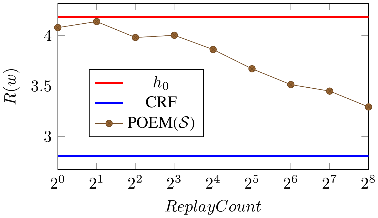
As we collect more data under $h_0$, our generalization error bound indicates that prediction performance should eventually approach that of the optimal hypothesis in the hypothesis space. We can simulate $n \rightarrow \infty$ by replaying the training data multiple times, collecting samples $y \sim h_0(\times)$. In the limit, we would observe every possible $y$ in the bandit feedback dataset, since $h_0(\times)$ has non-zero probability of exploring each prediction $y$. However, the learning rate may be slow, since the exponential model family has very thin tails, and hence may not be an ideal logging distribution to learn from. Holding all other details of the experiment setup fixed, we vary the number of times we replayed the training set ($ReplayCount$) to collect samples from $h_0$, and report the performance of POEM($\mathcal{S}$) on the Yeast dataset in Figure 1.

6.5 How does quality of $h_0$ affect learning?

In this experiment, we change the fraction of the training set $f \cdot n_{train}$ that was used to train the logging policy; as $f$ is increased, the quality of $h_0$ improves. Intuitively, there's a trade-off: better $h_0$ probably samples correct predictions more often and so produces a higher quality ${\cal D}$ to learn from, but it should also be harder to beat $h_0$.

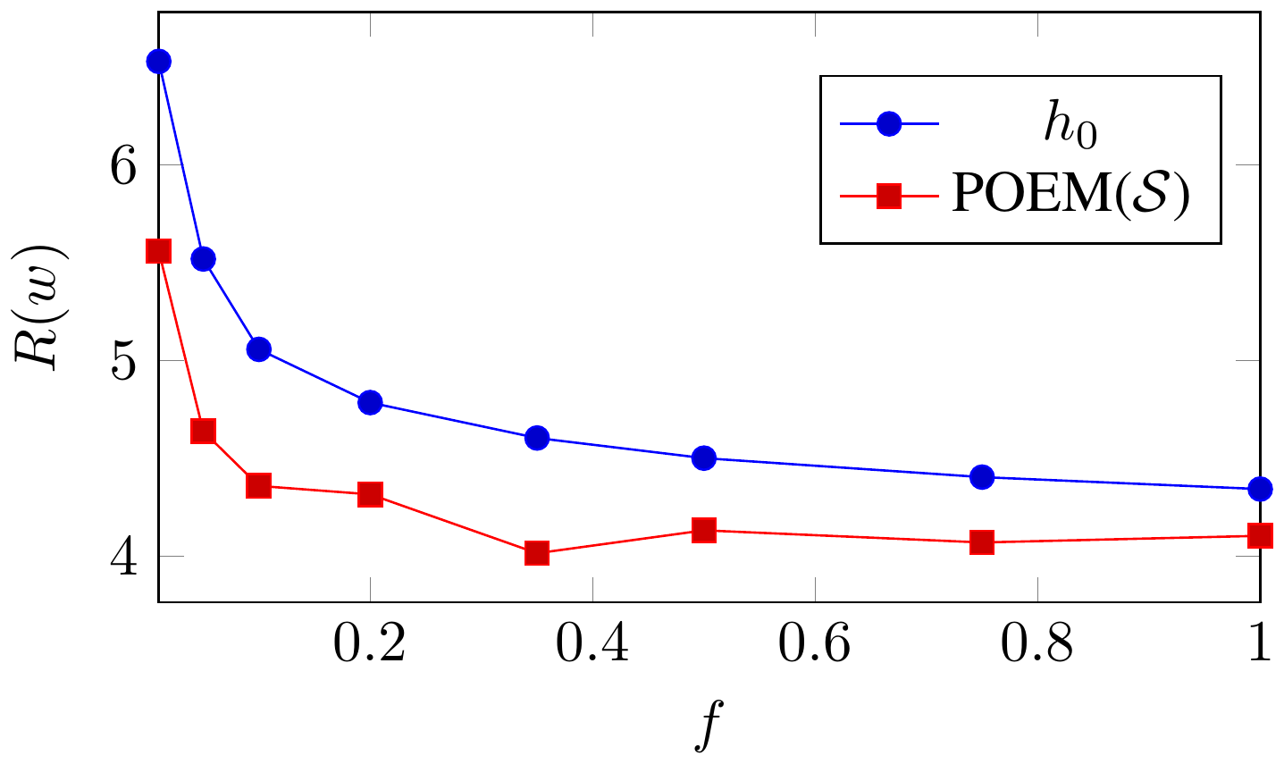
We vary $f$ from $1%$ to $100%$ while keeping all other conditions identical to the original experiment setup in Figure 2, and find that POEM($\mathcal{S}$) is able to consistently find a hypothesis at least as good as $h_0$. Moreover, even ${\cal D}$ collected from a poor quality $h_0$ ($0.5 \le f \le 0.2$) allows POEM($\mathcal{S}$) to effectively learn an improved policy.

6.6 How does stochasticity of $h_0$ affect learning?

Finally, the theory suggests that counterfactual learning is only possible when $h_0$ is sufficiently stochastic (the generalization bounds hold with high probability in the samples drawn from $h_0$). Does CRM degrade gracefully when this assumption is violated? We test this by introducing the temperature multiplier $w \mapsto \alpha w, \alpha > 0$ (as discussed in Section 5) into the logging policy. For $h_0 = h_{w_0}$, we scale $w_0 \mapsto \alpha w_0$, to derive a "more deterministic" variant of $h_0$, and generate ${\cal D} \sim h_{\alpha w_0}$. We report the performance of POEM($\mathcal{S}$) on the LYRL dataset in Figure 3 as we change $\alpha \in \left[0.5, \dots, 32\right]$, compared against $h_0$, and the deterministic predictor – $h_0\ map$ – derived from $h_0$. So long as there is some minimum amount of stochasticity in $h_0$, POEM($\mathcal{S}$) is still able to find a $w$ that improves upon $h_0$ and $h_0\ map$. The margin of improvement is typically greater when $h_0$ is more stochastic. Even when $h_0$ is too deterministic ($\alpha \ge 2^4$), performance of POEM($\mathcal{S}$) simply recovers $h_0 \ map$, suggesting that the CRM principle indeed achieves robust learning.

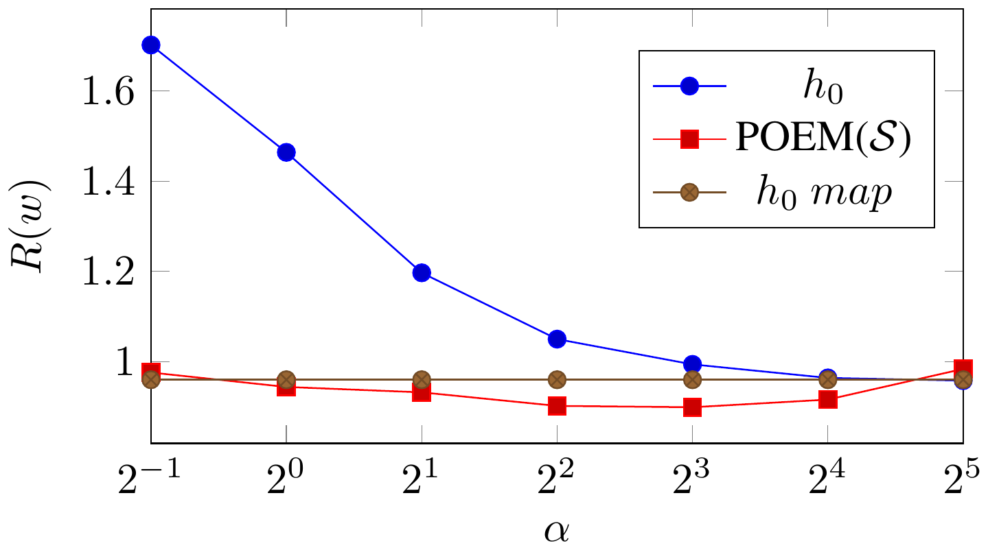
We observe the same trends (Figure 1, Figure 2 and Figure 3) across all datasets and optimization variants. They also remain unchanged when we include $l2-$ regularization (analogous to supervised CRFs to capture the capacity of ${\cal H}_{lin}$).

7. Conclusion

Section Summary: Counterfactual risk minimization provides a reliable way to train models from batches of logged interaction data by expanding the model space to include randomized decision rules, controlling variance in performance estimates, and adding a data-driven regularizer that prevents overfitting. Building on this idea, the authors created POEM, an algorithm that learns rich structured prediction policies as efficiently as standard supervised methods even when the output space is very large. The same principle also extends to ordinary supervised learning with complex, non-differentiable loss functions and points toward future refinements that handle noisy or interactive feedback.

Counterfactual risk minimization serves as a robust principle to design algorithms that can learn from a batch of bandit feedback interactions. The key insight for CRM is to expand the classical notion of a hypothesis class to include stochastic policies, reason about variance in the risk estimator, and derive a generalization error bound over this hypothesis space. The practical take-away is a simple, data-dependent regularizer that guarantees robust learning. Following the CRM principle, we developed POEM for structured output prediction. POEM can optimize over rich policy families (exponential models corresponding to linear rules in supervised learning), and deal with massive output spaces as efficiently as classical supervised methods.

The CRM principle more generally applies to supervised learning with non-differentiable losses, since the objective does not require the gradient of the loss function. We also foresee extensions of this work that relax some of the assumptions, e.g., to handle noisy ${\delta}(\cdot, \cdot)$, and ordinal or co-active feedback, or adaptive $h_0$ etc.

8. Acknowledgement

Section Summary: This research received partial funding from the National Science Foundation via two awards, along with support from the JTCII Cornell-Technion Research Fund and a gift from Bloomberg. The authors thank Chenhao Tan, Karthik Raman, and Vikram Rao for reviewing an early version of their paper. They also appreciate the anonymous conference reviewers for their helpful suggestions.

This research was funded in part through NSF Awards IIS-1247637 and IIS-1217686, the JTCII Cornell-Technion Research Fund, and a gift from Bloomberg. We thank Chenhao Tan, Karthik Raman and Vikram Rao for proofreading our manuscript, and the anonymous reviewers of ICML for their constructive feedback.

References

Section Summary: This section compiles a bibliography of academic papers and books primarily from the fields of machine learning and statistics. The works focus on techniques for evaluating decision-making algorithms using historical data, including contextual bandits for recommendations, counterfactual reasoning for assessing outcomes like ad clicks, and methods for safe or efficient policy learning. Additional references cover supporting areas such as optimization, causal inference, and theoretical foundations in statistical learning.

[1] Li, Lihong, Chu, Wei, Langford, John, and Schapire, Robert E. A contextual-bandit approach to personalized news article recommendation. In Proceedings of the 19th International Conference on World Wide Web, pp. 661–670, 2010.

[2] Bottou, Léon, Peters, Jonas, Candela, Joaquin Q., Charles, Denis X., Chickering, Max, Portugaly, Elon, Ray, Dipankar, Simard, Patrice Y., and Snelson, Ed. Counterfactual reasoning and learning systems: the example of computational advertising. Journal of Machine Learning Research, 14(1):3207–3260, 2013.

[3] Langford, John, Li, Lihong, and Dudík, Miroslav. Doubly robust policy evaluation and learning. In Proceedings of the 28th International Conference on Machine Learning, pp. 1097–1104, 2011.

[4] Li, Lihong, Chu, Wei, Langford, John, and Wang, Xuanhui. Unbiased offline evaluation of contextual-bandit-based news article recommendation algorithms. In Proceedings of the 4th ACM International Conference on Web Search and Data Mining, pp. 297–306, 2011.

[5] Li, Lihong, Chen, Shunbao, Kleban, Jim, and Gupta, Ankur. Counterfactual estimation and optimization of click metrics for search engines. CoRR, abs/1403.1891, 2014.

[6] Vapnik, V. Statistical Learning Theory. Wiley, Chichester, GB, 1998.

[7] Maurer, Andreas and Pontil, Massimiliano. Empirical bernstein bounds and sample-variance penalization. In Proceedings of the 22nd Conference on Learning Theory, 2009.

[8] Duchi, John, Hazan, Elad, and Singer, Yoram. Adaptive subgradient methods for online learning and stochastic optimization. Journal of Machine Learning Research, 12:2121–2159, 2011.

[9] Beygelzimer, Alina and Langford, John. The offset tree for learning with partial labels. In Proceedings of the 15th ACM SIGKDD International Conference on Knowledge Discovery and Data Mining, pp. 129–138, 2009.

[10] Zadrozny, Bianca, Langford, John, and Abe, Naoki. Cost-sensitive learning by cost-proportionate example weighting. In Proceedings of the Third IEEE International Conference on Data Mining, pp. 435–, 2003.

[11] Rosenbaum, Paul R. and Rubin, Donald B. The central role of the propensity score in observational studies for causal effects. Biometrika, 70(1):41–55, 1983.

[12] Strehl, Alexander L., Langford, John, Li, Lihong, and Kakade, Sham. Learning from logged implicit exploration data. In Proceedings of the 24th Annual Conference on Neural Information Processing Systems, pp. 2217–2225, 2010.

[13] Li, Lihong, Munos, Remi, and Szepesvari, Csaba. Toward minimax off-policy value estimation. In Proceedings of the 18th International Conference on Artificial Intelligence and Statistics (AISTATS), 2015.

[14] Thomas, Philip S., Theocharous, Georgios, and Ghavamzadeh, Mohammad. High-confidence off-policy evaluation. In Proceedings of the 29th AAAI Conference on Artificial Intelligence, pp. 3000–3006, 2015.

[15] Langford, John, Strehl, Alexander, and Wortman, Jennifer. Exploration scavenging. In Proceedings of the 25th International Conference on Machine Learning, pp. 528–535, 2008.

[16] Mary, Jérémie, Preux, Philippe, and Nicol, Olivier. Improving offline evaluation of contextual bandit algorithms via bootstrapping techniques. In Proceedings of the 31st International Conference on Machine Learning, pp. 172–180, 2014.

[17] Galichet, Nicolas, Sebag, Michèle, and Teytaud, Olivier. Exploration vs exploitation vs safety: Risk-aware multi-armed bandits. In Asian Conference on Machine Learning, pp. 245–260, 2013.

[18] Langford, John and Zhang, Tong. The epoch-greedy algorithm for multi-armed bandits with side information. In Proceedings of the 21st Annual Conference on Neural Information Processing Systems, pp. 817–824, 2008.

[19] Garcia, J. and Fernandez, F. Safe exploration of state and action spaces in reinforcement learning. Journal of Artificial Intelligence Research, 45:515–564, 2012.

[20] Shivaswamy, Pannagadatta K. and Joachims, Thorsten. Multi-armed bandit problems with history. In Proceedings of the 15th International Conference on Artificial Intelligence and Statistics, pp. 1046–1054, 2012.

[21] Hofmann, Katja, Schuth, Anne, Whiteson, Shimon, and de Rijke, Maarten. Reusing historical interaction data for faster online learning to rank for IR. In Sixth ACM International Conference on Web Search and Data Mining, pp. 183–192, 2013.

[22] Ionides, Edward L. Truncated importance sampling. Journal of Computational and Graphical Statistics, 17(2):295–311, 2008.

[23] Anthony, Martin and Bartlett, Peter L. Neural Network Learning: Theoretical Foundations. Cambridge University Press, New York, NY, USA, 2009.

[24] Owen, Art B. Monte Carlo theory, methods and examples. 2013.

[25] Tsochantaridis, Ioannis, Hofmann, Thomas, Joachims, Thorsten, and Altun, Yasemin. Support vector machine learning for interdependent and structured output spaces. In Proceedings of the 21st International Conference on Machine Learning, pp. 104–, 2004.

[26] Lafferty, John D., McCallum, Andrew, and Pereira, Fernando C. N. Conditional random fields: Probabilistic models for segmenting and labeling sequence data. In Proceedings of the 18th International Conference on Machine Learning, pp. 282–289, 2001.

[27] Yu, Jin, Vishwanathan, S. V. N., Günter, Simon, and Schraudolph, Nicol N. A quasi-Newton approach to nonsmooth convex optimization problems in machine learning. Journal of Machine Learning Research, 11:1145–1200, 2010.

[28] Lewis, Adrian S. and Overton, Michael L. Nonsmooth optimization via quasi-newton methods. Mathematical Programming, 141(1-2):135–163, 2013.

[29] van den Burg, G.J.J. and Groenen, P.J.F. GenSVM: A Generalized Multiclass Support Vector Machine. Technical Report EI 2014-33, Erasmus University Rotterdam, Erasmus School of Economics (ESE), Econometric Institute, 2014.

[30] Agarwal, Alekh, Hsu, Daniel, Kale, Satyen, Langford, John, Li, Lihong, and Schapire, Robert. Taming the monster: A fast and simple algorithm for contextual bandits. In Proceedings of the 31st International Conference on Machine Learning, pp. 1638–1646, 2014.

[31] Blum, Avrim, Kalai, Adam, and Langford, John. Beating the hold-out: Bounds for k-fold and progressive cross-validation. In Proceedings of the Twelfth Annual Conference on Computational Learning Theory, pp. 203–208, 1999.

[32] Pedregosa, F., Varoquaux, G., Gramfort, A., Michel, V., Thirion, B., Grisel, O., Blondel, M., Prettenhofer, P., Weiss, R., Dubourg, V., Vanderplas, J., Passos, A., Cournapeau, D., Brucher, M., Perrot, M., and Duchesnay, E. Scikit-learn: Machine learning in Python. Journal of Machine Learning Research, 12:2825–2830, 2011.