Residual Koopman Spectral Profiling

for Predicting and Preventing Transformer Training Instability

Bum Jun Kim $^{1}$, Shohei Taniguchi $^{1}$, Makoto Kawano $^{1}$, Yusuke Iwasawa $^{1}$, Yutaka Matsuo $^{1}$

$^{1}$ Graduate School of Engineering, The University of Tokyo, Japan

Abstract

Training divergence in transformers wastes compute, yet practitioners discover instability only after expensive runs begin. They therefore need an expected probability of failure for a transformer before training starts. Our study of Residual Koopman Spectral Profiling (RKSP) provides such an estimate. From a single forward pass at initialization, RKSP extracts Koopman spectral features by applying whitened dynamic mode decomposition to layer-wise residual snapshots. Our central diagnostic, the near-unit spectral mass, quantifies the fraction of modes concentrated near the unit circle, which captures instability risk. For predicting divergence across extensive configurations, this estimator achieves an AUROC of 0.995, outperforming the best gradient baseline. We further make this diagnostic actionable through Koopman Spectral Shaping (KSS), which reshapes spectra during training. We empirically validate that our method works in practice: RKSP predicts divergence at initialization, and when RKSP flags high risk, turning on KSS successfully prevents divergence. In the challenging high learning rate regime without normalization layers, KSS reduces the divergence rate from 66.7% to 12.5% and enables learning rates that are 50% to 150% higher. These findings generalize to WikiText-103 language modeling, vision transformers on CIFAR-10, and pretrained language models, including GPT-2 and LLaMA-2 up to 7B, as well as emerging architectures such as MoE, Mamba-style SSMs, and KAN.

Executive Summary: Training large transformer models often fails due to sudden divergence that wastes significant compute. Practitioners typically discover instability only after runs have already started, leaving them without reliable ways to assess risk in advance or adjust training proactively.

This work set out to develop a practical method for estimating the probability that a given transformer configuration will diverge before any training begins, and to turn that estimate into an intervention that prevents failure while allowing more aggressive optimization.

The authors analyzed residual streams in transformers as discrete dynamical systems. They collected a modest number of activation snapshots from a single forward pass at initialization, applied whitened dynamic mode decomposition to each layer, and extracted spectral features. The central diagnostic is near-unit spectral mass, which measures how many modes lie close to the unit circle. They also introduced a spectral regularizer, applied during training, that steers eigenvalues away from unstable regions. Experiments spanned normalization strategies, learning-rate regimes, model sizes up to 350 million parameters, language-modeling and vision tasks, and several emerging architectures.

The spectral diagnostic predicted divergence with an area under the ROC curve of 0.995 across dozens of configurations, substantially outperforming gradient-based baselines. When the diagnostic flagged high risk, the regularizer reduced observed divergence from roughly two-thirds of runs to about one-eighth and permitted learning rates 50–150 percent higher while preserving stability. The same patterns held on WikiText-103, vision transformers, and models up to 7 billion parameters, as well as on mixture-of-experts, state-space, and Kolmogorov–Arnold networks.

These results matter because they convert an expensive trial-and-error process into a low-cost pre-training check and a lightweight training adjustment. Organizations can prune risky hyperparameter choices early, avoid wasted GPU hours, and safely adopt larger step sizes that shorten training time. The approach also supplies a mechanistic explanation for why some normalization schemes and initializations succeed or fail.

Senior leaders should adopt the initialization-time spectral check as a standard gate before large-scale runs and enable the spectral regularizer whenever the check indicates elevated risk. When further validation is required, a small pilot on representative workloads will confirm overhead and calibration for the specific environment.

The method assumes that a linear approximation of each layer remains informative and that moderate deviations from normality do not dominate behavior; calibration between predicted and observed risk is only moderate. Results are strongest in the regimes tested and may need re-tuning of thresholds when applied to substantially different model families or optimizers.

Residual Koopman Spectral Profiling

for Predicting and Preventing Transformer Training Instability (Supplementary Material)

1. Introduction

Section Summary: Transformers can exhibit sudden training failures like exploding gradients that waste significant compute, since problems often appear only after expensive runs have already started. The authors introduce Residual Koopman Spectral Profiling, a method that treats each layer as a simple dynamical system and extracts a stability signal from one forward pass, yielding a probability-like score that predicts divergence with very high accuracy. They also present a training adjustment called Koopman Spectral Shaping that modifies these signals to reduce instability and allow larger learning rates.

Transformers ([1]) exhibit unpredictable training dynamics despite stabilization techniques such as layer normalization ([2]) and careful initialization. In particular, exploding-gradient instability remains a known failure mode in deep networks ([3]). This unpredictability in training divergence wastes compute: practitioners often discover divergence only after expensive runs have begun. Addressing this problem requires a calibrated, initialization-time risk estimate, which enables early pruning of risky configurations. Such an estimate should output a probability that matches empirical frequency rather than a heuristic score.

To provide such estimates, we propose Residual Koopman Spectral Profiling (RKSP), which views transformer layers as discrete-time dynamical systems. From a single forward pass, RKSP applies whitened dynamic mode decomposition (DMD) ([4]) to estimate local linear operators that approximate the residual stream evolution $\mathbf{h}_0 \to \mathbf{h}_1 \to \cdots \to \mathbf{h}_L$. The resulting layer-wise spectra provide a compact, predictive summary of stability.

Intuitively, when a layer's local linearization is close to normal, eigenvalues near the unit circle imply near-isometric propagation and therefore weak damping of signals and gradients. In high learning rate regimes, such weak damping can leave perturbations and optimization noise to be less attenuated, increasing divergence risk; conversely, strongly contractive spectra tend to be more stable but may cause rapid gradient decay. We summarize this trade-off with the near-unit mass $M_{\approx 1}$, the fraction of modes near the unit circle, together with a separate measure of non-normality; Section 4 provides a theoretical explanation for this behavior.

The near-unit mass $M_{\approx 1}$ exhibits a strong instability signal; using the monotone risk score $M_{\approx 1}$ yields an Area Under the Receiver Operating Characteristic curve (AUROC) of 0.995 for divergence prediction across various normalization strategies, tasks, and architectures. To make this signal further actionable, we introduce Koopman Spectral Shaping (KSS), which reshapes spectra during training to reduce divergence.

Our contributions are as follows.

• We propose RKSP, which estimates layer-wise Koopman spectra at initialization via whitened DMD (Section 3.2).
• We propose KSS, which reshapes spectra during training, preventing instability and permitting larger learning rates (Section 3.3).
• We provide theoretical bounds linking near-unit mass, near-normality, and the trade-offs between instability and expressivity (Section 4).
• We validate RKSP across various normalization strategies, datasets, and architectures, including language models, vision transformer (ViT) models, and emerging neural network families (Section 5 and Appendix G).

2. Background

Section Summary: Transformers built from residual layers can be viewed as a sequence of discrete dynamical systems, where each layer applies an additive update that evolves the internal state forward in time. Koopman operator theory offers a linear lens on these nonlinear updates by lifting them into a higher-dimensional space whose eigenvalues reveal whether signals will grow, decay, or oscillate across layers; dynamic mode decomposition provides a practical way to estimate these eigenvalues from data. The section also surveys related ideas on critical initialization, edge-of-chaos behavior, and normalization-free training, framing the present work as a diagnostic that uses these spectral properties to forecast stability at initialization time.

A transformer with $L$ layers updates its residual stream according to the residual formulation ([5]):

$ \mathbf{h}{\ell+1} = \mathbf{h}\ell + f_\ell(\mathbf{h}\ell; \theta\ell) = F_\ell(\mathbf{h}_\ell),\tag{1} $

where $f_\ell$ comprises self-attention or multi-layer perceptron sub-layers. This formulation reveals that each layer transition defines a discrete-time dynamical system. Also, residual networks can be viewed as discretizations of continuous-time dynamical systems, motivating stability analysis from an ordinary differential equation perspective ([6, 7]). Indeed, the local linearization of this system characterizes its stability.

2.1 Koopman Operator Theory and DMD Primer

Consider a discrete-time dynamical system $\mathbf{x}_{t+1} = F(\mathbf{x}_t)$ on state space $\mathcal{X} \subseteq \mathbb{R}^d$. The Koopman operator $\mathcal{K}: \mathcal{F} \to \mathcal{F}$ acts on observable functions $g: \mathcal{X} \to \mathbb{C}$ via composition with the dynamics ([8, 9, 10, 4]):

$ (\mathcal{K}g)(\mathbf{x}) \triangleq g(F(\mathbf{x})).\tag{2} $

For a nonlinear $F$, the operator $\mathcal{K}$ is infinite-dimensional but remains linear regardless of the nonlinearity in $F$. The spectral properties of $\mathcal{K}$ —its eigenvalues ${\lambda_j}$ and eigenfunctions ${\phi_j}$ —encode the intrinsic timescales and geometric structure of the dynamics:

$ \begin{aligned} \mathcal{K}\phi_j & = \lambda_j \phi_j, \ \text{therefore } \phi_j(F^n(\mathbf{x})) & = \lambda_j^n \phi_j(\mathbf{x}), \text{for all } n \geq 0. \end{aligned}\tag{3} $

The spectrum admits direct interpretation: modes with $|\lambda_j| > 1$ grow exponentially, modes with $|\lambda_j| < 1$ decay exponentially, and modes with $|\lambda_j| = 1$ persist or oscillate. The argument $\arg(\lambda_j)$ gives the oscillation frequency of mode $j$ ([11]).

In a layer-wise, non-autonomous setting, each layer has its own distinct operator, so each $\hat{\mathbf{A}}\ell$ must be estimated separately. Thus, the modulus $|\lambda(\hat{\mathbf{A}}\ell)|$ indicates a local, per-layer expansion or contraction tendency. DMD approximates these layer-wise Koopman operators from finite data ([12, 4, 13]).

2.2 Related Work

Koopman methods in machine learning.

Existing Koopman methods approximate operators via DMD and its extensions or learn linearizing transformations for dynamics prediction ([14, 15, 16]). These methods primarily target representation learning.

Edge of chaos.

The edge of chaos hypothesis links optimal trainability to critical initialization and signal propagation regimes ([17, 18, 19]), where signals neither explode nor vanish.

Neural tangent kernel.

The neural tangent kernel characterizes gradient descent in the infinite-width limit and yields kernel-regression behavior ([20]). In particular, linearizing the network around its initialization makes the kernel essentially constant, so training reduces to regression with this fixed kernel.

Mean-field theory and $\mu$ P.

Mean-field theory and Maximal Update Parameterization ($\mu$ P) enable hyperparameter transfer across scales through asymptotic analysis ([17, 21]).

Normalization-free training.

Normalization-free residual networks can be stabilized with Fixup initialization ([22]). ReZero trains deep residual networks and transformers without normalization by introducing a residual scaling parameter initialized to zero, so the network starts near an identity map ([23]). Normalizer-Free Networks replace normalization with scaled activations and adaptive gradient clipping, enabling stable large-scale training without normalization layers ([24]). We discuss Fixup and ReZero-style identity initialization through the RKSP lens in Appendix J.

Positioning of this study.

RKSP uses Koopman spectra as an initialization-time diagnostic: from a single forward pass, we estimate layer-wise operators and predict divergence risk. Unlike Koopman representation learning for forecasting ([14, 15, 16]), our near-unit mass $M_{\approx 1}$ provides a measurable handle on critical signal propagation ([17, 18, 19]) and captures instabilities beyond neural tangent kernel analyses ([20]); we make it actionable via KSS and validate it in no-normalization regimes ([22, 24]).

3. Method

Section Summary: The method predicts whether a neural network training run will diverge by first defining divergence as a loss above 50 or gradient norm above 500, then collecting residual activation snapshots from a single forward pass at initialization. These snapshots are processed layer by layer through a whitened dynamic mode decomposition procedure that approximates each layer transition with a linear operator and extracts spectral features such as radius, eigenvector condition number, Kreiss constant, and a nonlinearity ratio. The resulting profile is fed to a probabilistic model that estimates divergence probability before any training begins.

3.1 Problem Setup

Divergence Definition

A training run is marked as diverged if, at any step, the loss exceeds 50.0 or the gradient norm exceeds 500.0. This criterion defines the binary label $D \in {0, 1}$ used throughout our experiments.

Divergence Prediction Task

Given a model architecture, normalization strategy, optimizer choice, and dataset, we collect $N$ residual-stream snapshots at initialization from a single forward pass and compute the spectral profile $\mathcal{S}$. A probabilistic predictor then maps $\mathcal{S}$ to $P(D=1 \mid \mathcal{S})$, estimating divergence risk before training begins.

3.2 Residual Koopman Spectral Profiling

Algorithm 1 summarizes our RKSP procedure. The algorithm computes DMD for each layer to obtain its spectral profile: $\rho_\ell$ denotes the spectral radius of $\hat{\mathbf{A}}\ell$, $\kappa\ell$ the eigenvector condition number of its eigenbasis, and $\mathcal{K}_\ell$ the Kreiss constant (Appendix B).

Require: Model $\mathcal{M}$ with $L$ layers; dataset $\mathcal{D}$; the number of samples $N$
Ensure: Spectral profile $\mathcal{S} = \{(M_{\approx 1}^\ell, \rho_\ell, \kappa_\ell, \eta_{\mathrm{nl}}^\ell, \mathcal{K}_\ell)\}_{\ell=0}^{L-1}$
Collect residuals: for each batch $\mathbf{x} \in \mathcal{D}$, store $\{\mathbf{h}_\ell(\mathbf{x})\}_{\ell=0}^L$
for $\ell = 0, \ldots, L-1$ do
  Form snapshot matrices $\mathbf{X}_\ell, \mathbf{Y}_\ell \in \mathbb{R}^{d \times N}$
  Whitening: $\tilde{\mathbf{X}}_\ell = \hat{\boldsymbol{\Sigma}}_\ell^{-1/2}(\mathbf{X}_\ell - \bar{\mathbf{X}}_\ell)$, $\tilde{\mathbf{Y}}_\ell = \hat{\boldsymbol{\Sigma}}_\ell^{-1/2}(\mathbf{Y}_\ell - \bar{\mathbf{Y}}_\ell)$
  DMD: $\hat{\mathbf{A}}_\ell = \tilde{\mathbf{Y}}_\ell \tilde{\mathbf{X}}_\ell^\dagger$
  Eigendecomposition: $\hat{\mathbf{A}}_\ell = \mathbf{V}_\ell \boldsymbol{\Lambda}_\ell \mathbf{V}_\ell^{-1}$
  Compute $M_{\approx 1}^\ell, \rho_\ell, \kappa_\ell$, nonlinearity $\eta_{\mathrm{nl}}^\ell$, Kreiss $\mathcal{K}_\ell$
end for
Aggregate mean, max, min, std across layers
return $\mathcal{S}$

3.2.1 Snapshot Construction

RKSP applies DMD to each layer transition $\mathbf{h}\ell \to \mathbf{h}{\ell+1}$ as described . Let ${\mathbf{x}i}{i=1}^N$ denote the $N$ inputs used to form the snapshots. For layer $\ell$, define the paired residual vectors $\mathbf{x}i^{(\ell)} = \mathbf{h}\ell(\mathbf{x}_i)$ and $\mathbf{y}i^{(\ell)} = \mathbf{h}{\ell+1}(\mathbf{x}_i)$. The snapshot matrices are

$ \begin{aligned} \mathbf{X}_\ell & = [\mathbf{x}_1^{(\ell)}, \ldots, \mathbf{x}N^{(\ell)}], \ \mathbf{Y}\ell & = [\mathbf{y}_1^{(\ell)}, \ldots, \mathbf{y}_N^{(\ell)}] \in \mathbb{R}^{d \times N}, \end{aligned}\tag{4} $

so each column pair corresponds to the same sample. Unlike standard DMD, which uses time-shifted trajectories, RKSP pairs columns across different samples. Concretely, column $i$ in $\mathbf{X}$ is the residual snapshot $\mathbf{h}_\ell(\mathbf{x}i)$ and column $i$ in $\mathbf{Y}$ is the corresponding next-layer snapshot $\mathbf{h}{\ell+1}(\mathbf{x}_i)$ for the same sample $\mathbf{x}i$; columns index independent samples, not time steps of a single trajectory. For each layer, DMD yields a local linear approximation $\hat{\mathbf{A}}\ell$ whose spectrum characterizes the dynamics at that depth.

To quantify how well this linear approximation fits the data, we define the nonlinearity ratio in whitened coordinates:

$ \eta_{\mathrm{nl}}(\ell) \coloneqq \frac{\left|\tilde{\mathbf{Y}}\ell - \hat{\mathbf{A}}\ell \tilde{\mathbf{X}}\ell\right|F}{\left|\tilde{\mathbf{Y}}\ell - \tilde{\mathbf{X}}\ell\right|F + \varepsilon{\mathrm{nl}}},\tag{5} $

where $\varepsilon_{\mathrm{nl}} > 0$ is a small constant that prevents division by zero. This ratio $\eta_{\mathrm{nl}}$ normalizes the fit error by the update magnitude. When the residual update $\left|\tilde{\mathbf{Y}}\ell-\tilde{\mathbf{X}}\ell\right|F$ is tiny, $\eta{\mathrm{nl}}$ can be large even for small absolute errors. We therefore use $\eta_{\mathrm{nl}}$ primarily as a DMD reliability flag rather than as a pure measure of nonlinearity.

3.2.2 Whitened DMD and Reliability Filtering

DMD approximates the Koopman operator from data snapshots. Given paired snapshot matrices $\mathbf{X} = [\mathbf{x}_1, \ldots, \mathbf{x}_N] \in \mathbb{R}^{d \times N}$ and $\mathbf{Y} = [\mathbf{y}_1, \ldots, \mathbf{y}_N] \in \mathbb{R}^{d \times N}$, DMD solves for the optimal linear operator:

$ \hat{\mathbf{A}}{\mathrm{DMD}} = \operatorname{argmin}{\mathbf{A} \in \mathbb{R}^{d \times d}} \left|\mathbf{Y} - \mathbf{A}\mathbf{X}\right|_F^2 = \mathbf{Y}\mathbf{X}^\dagger,\tag{6} $

where $\mathbf{X}^\dagger$ denotes the Moore-Penrose pseudoinverse.

To ensure scale-invariance and numerical stability, we apply $\mathbf{X}$-based zero-phase component analysis whitening ([25]):

$ \begin{aligned} \tilde{\mathbf{X}} & = \hat{\boldsymbol{\Sigma}}_X^{-1/2}(\mathbf{X} - \bar{\mathbf{X}}\mathbf{1}^\top), \ \tilde{\mathbf{Y}} & = \hat{\boldsymbol{\Sigma}}_X^{-1/2}(\mathbf{Y} - \bar{\mathbf{Y}}\mathbf{1}^\top), \ \hat{\boldsymbol{\Sigma}}_X & = \frac{1}{N-1}(\mathbf{X} - \bar{\mathbf{X}}\mathbf{1}^\top)(\mathbf{X} - \bar{\mathbf{X}}\mathbf{1}^\top)^\top + \epsilon\mathbf{I} \end{aligned} $

where $\bar{\mathbf{X}} = \frac{1}{N}\sum_{i=1}^{N} \mathbf{x}i$, $\bar{\mathbf{Y}} = \frac{1}{N}\sum{i=1}^{N} \mathbf{y}_i$, and $\epsilon > 0$ ensures invertibility. The same whitening matrix is applied to both $\mathbf{X}$ and $\mathbf{Y}$, so the regression operates within a single, $\mathbf{X}$-normalized coordinate system. This whitening step ensures cross-model comparability and yields coordinate-invariant spectral estimates.

From the whitened data, we form the DMD operator $\hat{\mathbf{A}} = \tilde{\mathbf{Y}}\tilde{\mathbf{X}}^\dagger$ and compute its eigendecomposition $\hat{\mathbf{A}} = \mathbf{V}\boldsymbol{\Lambda}\mathbf{V}^{-1}$. To report the eigenvector condition number $\kappa(\mathbf{V}) = \left|\mathbf{V}\right|_2\left|\mathbf{V}^{-1}\right|_2$, we first normalize each right eigenvector to have unit Euclidean norm. This normalization fixes the otherwise arbitrary scaling of $\mathbf{V}$ and makes $\kappa(\mathbf{V})$ reproducible.

To identify spurious eigenvalues, we apply residual DMD (ResDMD) reliability filtering ([26]). For each eigenvalue $\lambda_j$ with left eigenvector $\mathbf{u}_j$ satisfying $\mathbf{u}_j^*\hat{\mathbf{A}} = \lambda_j \mathbf{u}_j^*$, we compute the per-mode residual:

$ r_j = \frac{\left|\mathbf{u}_j^*(\tilde{\mathbf{Y}} - \lambda_j \tilde{\mathbf{X}})\right|_2}{\left|\mathbf{u}_j^*\tilde{\mathbf{X}}\right|_2 + \varepsilon_r},\tag{7} $

where $\varepsilon_r > 0$ prevents division by zero. Eigenvalues with $r_j > \tau$ are flagged as unreliable and potentially spurious; we use a default threshold of $\tau = 0.1$ to filter them out.

3.2.3 Spectral Mass

Now, we define our criterion for divergence prediction.

########## {caption="Definition 1: Spectral Mass Partition"}

For DMD eigenvalues $\Lambda = {\lambda_j}_{j=1}^m$ of an operator $\hat{\mathbf{A}}$, with $m$ the number of eigenvalues used, we define the following bins; they are disjoint provided $\delta_c \ge \epsilon_n$:

$ \begin{aligned} M_{>1}(\hat{\mathbf{A}}) & \triangleq \frac{1}{m}\sum_{j=1}^m \mathbf{1}[|\lambda_j| > 1 + \epsilon_u], \ M_{\approx 1}(\hat{\mathbf{A}}) & \triangleq \frac{1}{m}\sum_{j=1}^m \mathbf{1}[|\lambda_j| \in [1-\epsilon_n, 1+\epsilon_u]], \ M_{<1}(\hat{\mathbf{A}}) & \triangleq \frac{1}{m}\sum_{j=1}^m \mathbf{1}[|\lambda_j| < 1 - \delta_c], \end{aligned} $

where the three quantities denote the expansive mass, near-unit mass, and contractive mass, respectively. When $\delta_c > \epsilon_n$, these three bins are not exhaustive; the remaining intermediate mass is $M_{\mathrm{mid}}(\hat{\mathbf{A}}) \triangleq 1 - M_{>1}(\hat{\mathbf{A}}) - M_{\approx 1}(\hat{\mathbf{A}}) - M_{<1}(\hat{\mathbf{A}})$.

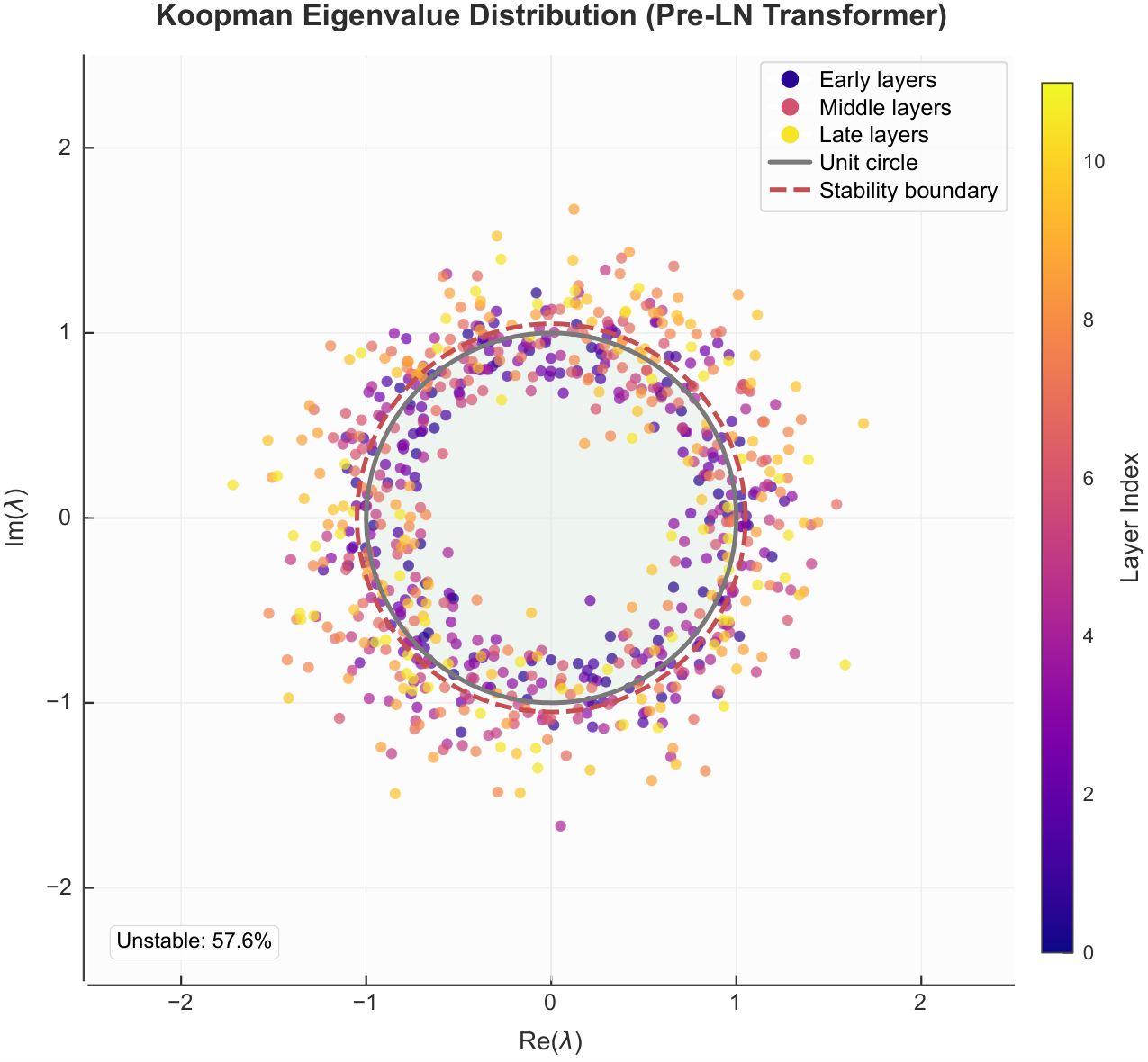
For example, $m=d$ for full DMD, $m=r$ for rank- $r$ randomized DMD ([27]), or $m$ equals the count remaining after reliability filtering. We use default thresholds $\epsilon_u = 0.05$, $\epsilon_n = 0.10$, and $\delta_c = 0.20$. Figure 1 shows a representative eigenvalue scatter that motivates these bins.

Metric Interpretation.

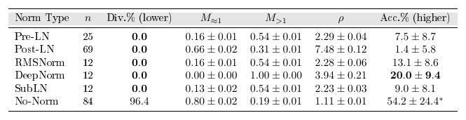
For divergence prediction, we use $M_{\approx 1}$ itself as the scalar score and compute the AUROC against the divergence labels. Note that the expansive mass $M_{>1}$ tracks eigenvalues outside the unit circle but does not map one-to-one with empirical divergence. Four factors explain this gap between $M_{>1}$ and observed divergence. First, whitening rescales local coordinates, so raw eigenvalue magnitudes differ from unwhitened values. Second, DMD provides only a local linear approximation of the true nonlinear dynamics. Third, non-normal transient growth can trigger instability even when few eigenvalues exceed 1 ([28]). Additionally, our divergence labels use coarse thresholds on loss or gradient norm, so finite-horizon training within the evaluation window can remain stable despite a nonzero $M_{>1}$. These four factors together explain cases like Pre-LN, which shows a nonzero $M_{>1}$ but 0% divergence in Table 1.

3.3 Koopman Spectral Shaping

While RKSP diagnoses instability, KSS prevents it. KSS adds a differentiable spectral regularizer to the training objective that steers eigenvalues away from the unstable region while reducing excessive near-unit mass to restore damping without causing over-contraction. The total objective becomes $\mathcal{L}{\mathrm{total}} = \mathcal{L}{\mathrm{task}} + \alpha \sum_{\ell \in \mathcal{S}} \mathcal{L}_{\mathrm{KSS}}^\ell / |\mathcal{S}|$, where $\mathcal{S}$ samples 50% of layers per update.

########## {caption="Definition 2: KSS Regularization Loss"}

For layer $\ell$ with randomized DMD eigenvalues ${\lambda_j^\ell}_{j=1}^r$, the KSS loss is

$ \begin{aligned}\mathcal{L}{\mathrm{KSS}}^\ell & = \underbrace{\sum{j=1}^r \sigma(T(|\lambda_j^\ell| - \tau_u)) \cdot \operatorname{softplus}(|\lambda_j^\ell| - \tau_u)^2}{\text{Unstable penalty}}\& + \underbrace{\beta \cdot (m\ell^{\mathrm{soft}} - \gamma)^2}_{\text{Near-unit target}}\end{aligned}\tag{8} $

where $\sigma(\cdot)$ denotes the sigmoid function and

$ m_\ell^{\mathrm{soft}} = \frac{1}{r}\sum_{j=1}^r \sigma(T(|\lambda_j^\ell| - \tau_l))\cdot \sigma(T(\tau_u - |\lambda_j^\ell|)).\tag{9} $

This term facilitates reducing excessive near-unit mass while preventing it from becoming too small by nudging $m_\ell^{\mathrm{soft}}$ toward the target band $\gamma$. We use the default hyperparameters $T = 20$, $\tau_u = 1.05$, $\tau_l = 0.90$, and $\gamma \in [0.3, 0.5]$. Full hyperparameter settings and the practical training recipe appear in Appendix D.

4. Theoretical Analysis

Section Summary: The near-unit mass is interpreted as an instability score because, for roughly normal matrices, a high fraction of eigenvalues clustered near magnitude one implies near-isometric signal propagation with little damping. This allows perturbations and optimization noise to persist or grow across depth, raising divergence risk in aggressive training regimes, as formalized by relating the expected squared norm of transformed vectors to the eigenvalue distribution. The same quantity governs depth-wise energy decay in linear networks under isotropic assumptions, though non-normality introduces transient growth effects that require tracking the eigenvector condition number as a caveat.

We interpret the near-unit mass $M_{\approx 1}$ as an instability score. Two mechanisms support this view. First, when the layer linearization is approximately normal, eigenvalues accurately reflect singular values, so concentration near $|\lambda|\approx 1$ implies near-isometric propagation and weak damping. Second, weak damping allows perturbations and optimization noise to persist across depth; in aggressive optimization regimes, this behavior raises divergence risk. We formalize the energy-preservation statement below and highlight non-normality as a caveat.

########## {caption="Theorem 3: Near-Unit Energy Preservation under Near-Normality"}

Let $\mathbf{A} \in \mathbb{C}^{d \times d}$ be normal with eigenvalues ${\lambda_j}_{j=1}^d$. For a unit vector $\mathbf{x}$ drawn uniformly on the sphere,

$ \mathbb{E} \left|\mathbf{A}\mathbf{x}\right|2^2 = \frac{1}{d}\sum{j=1}^d |\lambda_j|^2.\tag{10} $

If $\rho(\mathbf{A})\le 1+\epsilon_u$ and $M_{\approx 1}(\mathbf{A})$ denotes the fraction of eigenvalues with $|\lambda_j|\in [1-\epsilon_n, 1+\epsilon_u]$, then

$ (1-\epsilon_n)^2 M_{\approx 1}(\mathbf{A}) \le \mathbb{E} \left|\mathbf{A}\mathbf{x}\right|_2^2 \le (1+\epsilon_u)^2.\tag{11} $

Hence larger $M_{\approx 1}$ implies more energy-preserving and less damped propagation; this corresponds to higher instability risk. More generally, if $\mathbf{A}$ is diagonalizable with $\mathbf{A}=\mathbf{V}\boldsymbol{\Lambda}\mathbf{V}^{-1}$, then the same conclusion holds up to factors $\kappa(\mathbf{V})^{\pm 2}$:

$ \frac{(1-\epsilon_n)^2}{\kappa(\mathbf{V})^2} M_{\approx 1}(\mathbf{A}) \le \mathbb{E} \left|\mathbf{A}\mathbf{x}\right|_2^2 \le \kappa(\mathbf{V})^2(1+\epsilon_u)^2.\tag{12} $

########## {caption="Corollary 4: Depth-wise Damping and Gradient Flow"}

Consider a depth- $L$ linearization $\mathbf{h}{\ell+1}=\mathbf{A}\ell \mathbf{h}\ell$ where each $\mathbf{A}\ell$ is a normal and $\rho(\mathbf{A}\ell)\le 1+\epsilon_u$. Assume that each layer has an isotropic second moment, that is, $\mathbb{E}[\mathbf{h}\ell\mathbf{h}\ell^*] = \frac{1}{d}\mathbb{E}\left|\mathbf{h}\ell\right|2^2 \mathbf{I}$ for $\ell=0, \dots, L-1$. For example, $\frac{\mathbf{h}\ell}{\left|\mathbf{h}\ell\right|2}$ is uniform on the sphere. Let $q\ell \triangleq \frac{1}{d}\sum{j=1}^d |\lambda_j^\ell|^2$ be the average energy gain of layer $\ell$. Then

$ \mathbb{E}\left|\mathbf{h}_L\right|_2^2 = \mathbb{E}\left|\mathbf{h}0\right|2^2 \prod{\ell=0}^{L-1} q\ell,\tag{13} $

and $q_\ell \ge (1-\epsilon_n)^2 M_{\approx 1}(\mathbf{A}\ell)$. Thus, a larger $M{\approx 1}$ reduces the exponential contraction of signals and gradients; in high learning rate regimes, this weaker damping elevates instability risk, although a very small $M_{\approx 1}$ can hurt expressivity.

The proof appears in Appendix C.

Non-normality caveat.

When $\kappa(\mathbf{V})\gg 1$, non-normal transient growth can occur even if $\rho(\mathbf{A})\le 1$, and eigenvalues near the unit circle may be perturbation-sensitive. We therefore track $\kappa(\mathbf{V})$ alongside $M_{\approx 1}$. Appendix B and Appendix C characterize transient growth via the Kreiss theorem, provide normality-related bounds, and formalize the trade-off between instability and expressivity.

5. Experiments

Section Summary: The experiments evaluate a range of GPT-2-style transformer models, from 1M to 350M parameters, across six normalization strategies and multiple tasks including associative recall, language modeling, and image classification. They show that a spectral metric called M≈1 can predict training divergence at initialization with very high accuracy, far outperforming gradient-based baselines. A proposed regularization approach called KSS further improves stability by proactively shaping the spectrum, enabling higher learning rates, reducing divergence rates, and scaling effectively while outperforming methods like gradient clipping or generic regularization.

5.1 Experimental Settings

Our experiments target Generative Pretrained Transformer (GPT-2)-style transformers ([29, 1]) with $d \in {128, 256, 512, 768, 1024}$ and $L \in {4, 6, 8, 12, 16, 24}$, spanning 1M to 350M parameters. We compare six normalization strategies: pre-layer normalization (Pre-LN), post-layer normalization (Post-LN), root mean square normalization (RMSNorm) ([30]), DeepNorm ([31]), sub-layer normalization (SubLN) ([32]), and no normalization (No-Norm). The evaluation tasks include an associative-recall classification task (Appendix D.1); language modeling (LM) tasks including our synthetic LM with next-token prediction (Appendix D.2), WikiText-103 ([33]), and OpenWebText-style LM ([34]); and ViT experiments ([35]) on the Canadian Institute for Advanced Research (CIFAR-10) dataset ([36]). We report AUROC for discrimination, with 95% bootstrap confidence intervals (CIs) based on 1000 resamples. Statistical significance of divergence rates is assessed using Fisher's exact test and run with three random seeds per setting. Full hyperparameters and hardware details appear in Appendix D.

5.2 Prediction at Initialization

Main Results: Normalization Comparison.

Table 1 reveals three key findings. First, five of the six normalizations achieve 0\

::: {caption="Table 1: Comprehensive normalization comparison across different setups. RKSP metrics reveal distinct spectral signatures explaining stability differences. Accuracy is computed from only 3 converged runs out of 84. Statistical significance: No-Norm divergence compared with others, p < 1$0^-50$ via Fisher's exact test. AUROC for divergence prediction using $M_≈ 1 : 0.995 [95$% CI: 0.986 to 1.00]. Measured on the associative-recall task."}

:::

AUROC Analysis for Divergence Prediction.

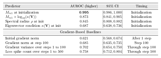
Table 2 compares spectral predictors against gradient baselines. We use the monotone risk score $M_{\approx 1}$ for divergence prediction. This achieves an AUROC of 0.995 at initialization, representing a 31\

::: {caption="Table 2: AUROC for divergence prediction with bootstrap 95% confidence intervals. The $M_≈ 1$ CI lower bound of 0.986 exceeds gradient baselines' upper bounds. Measured on the associative-recall normalization sweep."}

:::

5.3 Effect of KSS on Stability

KSS Results.

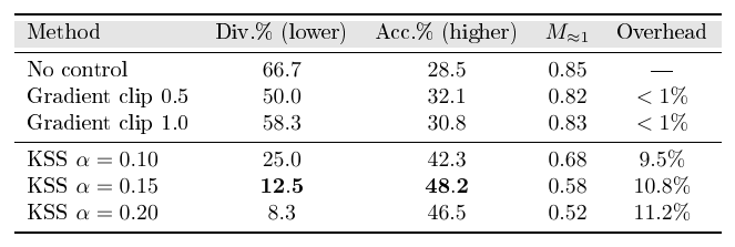
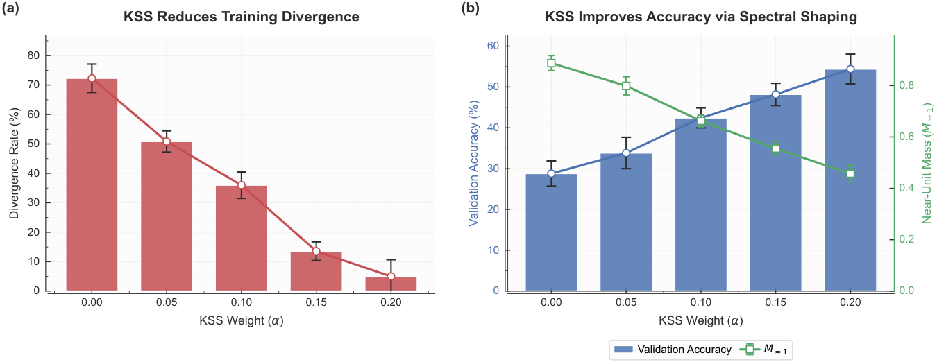
Table 3 compares gradient clipping with KSS in the No-Norm setting. These two approaches differ fundamentally in their mechanism. Gradient clipping operates reactively: it caps gradients after explosion begins but does not prevent instability, yielding only modest improvements. KSS, in contrast, operates proactively by shaping the spectral distribution before instability occurs. With $\alpha = 0.15$, KSS reduces divergence from 66.7\

::: {caption="Table 3: Gradient clipping versus KSS in a challenging No-Norm setting with learning rate that ranges from 0.005 to 0.01 and 24 trials each. Measured on the associative-recall task."}

:::

Extended Baseline Comparison.

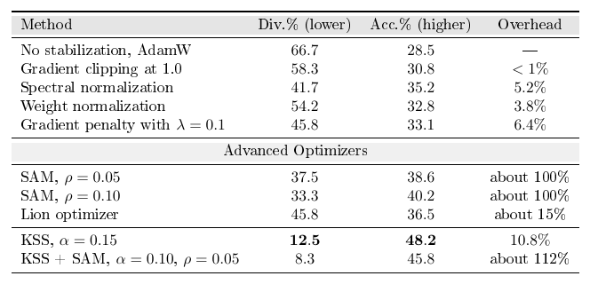
Table 4 provides expanded baseline and optimizer results, including spectral normalization and weight normalization baselines ([37, 38]). We use Adam with decoupled weight decay (AdamW) as the base optimizer in this comparison. Sharpness-Aware Minimization (SAM) ([39]) reduces divergence to 33.3\

::: {caption="Table 4: Extended baseline comparison including SAM, spectral normalization, and the Lion optimizer. Measured on the associative-recall task."}

:::

KSS Enables Higher Learning Rates.

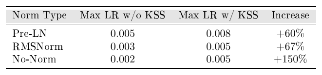
By suppressing spectral instability, KSS allows us to safely increase the step size across different normalization choices. Table 5 shows a 50\

::: {caption="Table 5: Maximum stable learning rate (LR). KSS enables learning rates that are 50% to 150% higher. The stability criterion is <20% divergence across trials. Measured on the associative-recall task."}

:::

Mechanistic Evidence: KSS versus Random Regularization.

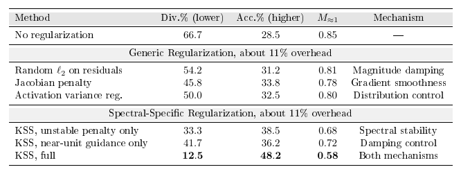
KSS stabilizes training through spectral shaping rather than generic regularization. Table 6 addresses this point via ablation studies with matched computational overhead. Generic regularization reduces divergence by only 20\

::: {caption="Table 6: Mechanism ablation: KSS versus random regularization. Same overhead at about 11%, different mechanisms. Results use the No-Norm setting, with learning rates ranging from 0.005 to 0.01 across 24 trials each. All methods are matched to about 11% computational overhead. Measured on the associative-recall task."}

:::

Scaling Analysis.

Table 7 extends KSS to 350M parameters. At this scale, KSS maintains sub-linear overhead scaling at 11.8\

::: {caption="Table 7: Scale-up KSS training results up to 350M parameters. Measured on the synthetic LM validation set with 24 trials on a synthetic LM task with vocab size 10K and a sequence length of 256."}

:::

5.4 Real-World LM Validation

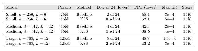
RKSP and KSS generalize beyond synthetic tasks to real-world LMs. Table 8 demonstrates this generalization with WikiText-103 ([33]) and OpenWebText experiments. Benefits with KSS persist on real data, manifesting in three ways. First, divergence decreases by 2 $\times$ to 5 $\times$ across model sizes. Second, KSS-trained models achieve 5\

::: {caption="Table 8: KSS improves stability and PPL. Pre-LN normalization with 24 trials per configuration. Measured on WikiText-103 and OpenWebText language-modeling tasks."}

:::

5.5 ViT Experiments

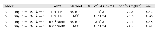
RKSP generalizes to ViTs ([35]), as Table 9 confirms. The spectral signatures transfer directly: ViT exhibits similar $M_{\approx 1}$ patterns to language transformers. KSS improves ViT training, yielding 3\

::: {caption="Table 9: ViT RKSP analysis and KSS training. Results use 24 trials, with an image size of 224, a patch size of 16, and a 5-epoch sanity check. Measured on CIFAR-10."}

:::

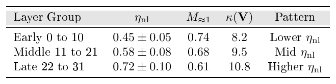
::: {caption="Table 10: LLaMA-2-7B analysis. The pattern persists at the 7B scale with RMSNorm. Computed from residual-stream activations on a fixed set of short prompt sentences. Measured on a fixed short-prompt set."}

:::

5.6 Large-Scale Pretrained Model Analysis

We further validate RKSP on large-scale pretrained language models. Appendix G provides additional tables and plots.

Large Language Model Meta AI 2 (LLaMA-2) 7B Analysis.

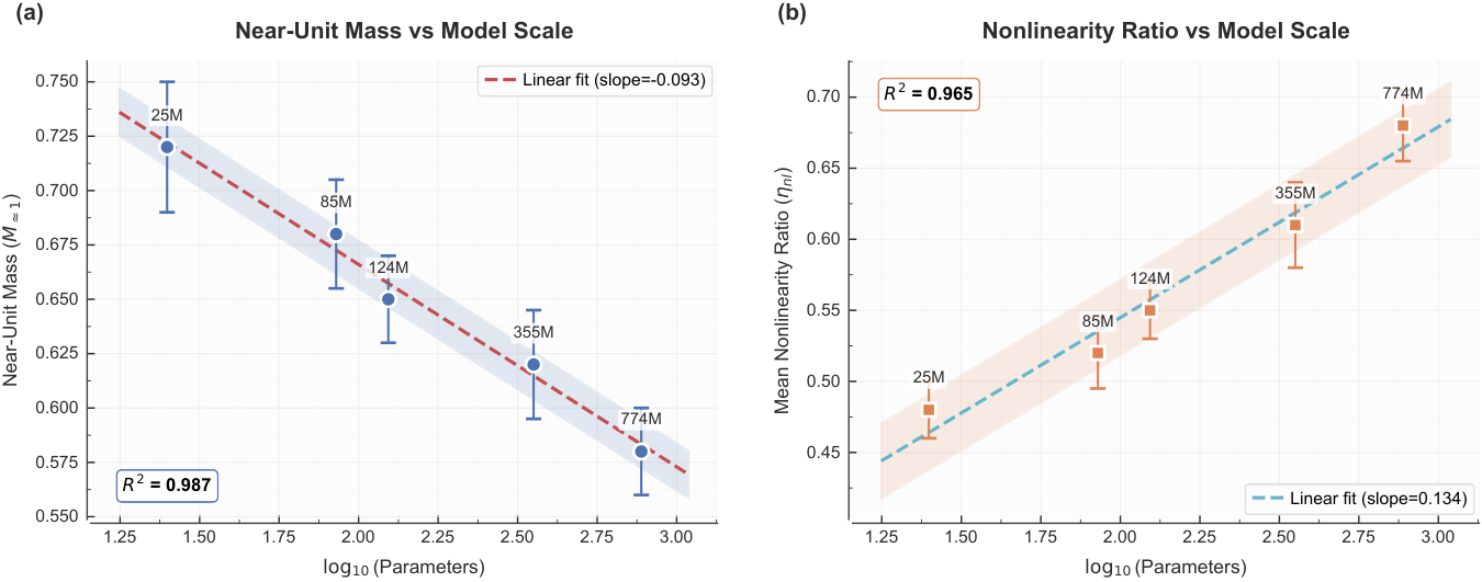
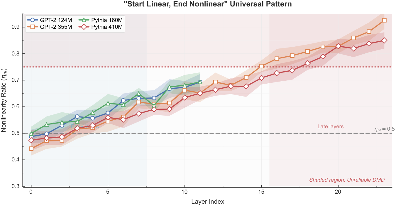
Table 10 extends our analysis to the 7B scale for LLaMA-2 ([41]). The Start Linear, End Nonlinear pattern persists at this scale: $\eta_{\mathrm{nl}}$ increases monotonically with depth, ranging from $0.45 \pm 0.05$ in the early layers to $0.72 \pm 0.10$ in the late layers. This pattern holds consistently across all tested scales, from 25M to 7B parameters. Figure 3 quantifies this relationship through scaling law analysis.

Beyond Transformers.

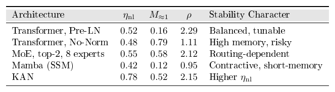
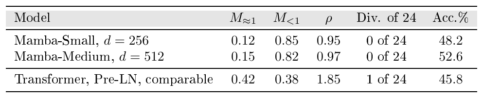
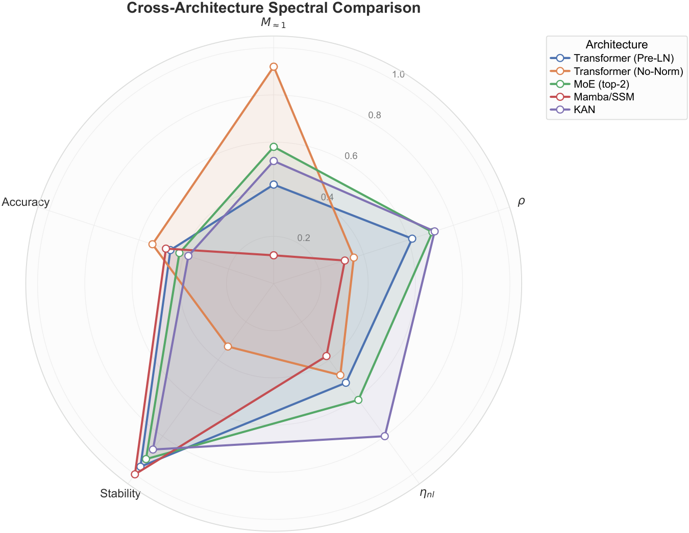
RKSP and KSS generalize beyond standard transformers to emerging architectures. We validate on Mixture of Experts (MoE) ([42]), Mamba-style state space model (SSM) architectures ([43]), and Kolmogorov-Arnold Networks (KAN) ([44]). Table 11 summarizes their characteristic spectral signatures: Mamba exhibits strongly contractive dynamics with low near-unit mass $M_{\approx 1}$, while MoE routing and KAN introduce higher nonlinearity and intermediate near-unit structure. Detailed case studies and additional comparisons appear in Appendix I.

::: {caption="Table 11: Cross-architecture spectral comparison. Transformer rows use the synthetic associative-recall task with seq len 64, vocab 256, and $n_p$airs=4; MoE, Mamba, and KAN rows use the synthetic LM task with random-token next-token prediction."}

:::

6. Conclusion

Section Summary: Researchers developed a diagnostic tool called RKSP that analyzes a transformer's initial state to forecast whether its training will diverge, achieving very high accuracy and allowing practitioners to abandon doomed runs early. They also created a regularization technique, KSS, that reshapes the model's internal dynamics to curb instability while preserving useful learning behavior, working alongside existing stabilization methods. Supporting theory shows why certain spectral patterns promote or prevent divergence, and these patterns hold across many models and training setups.

We introduced RKSP, a method that uses whitened DMD to estimate layer-wise residual dynamics and predict transformer training divergence before optimization begins. At initialization, the risk score $M_{\approx 1}$ achieves an AUROC of 0.995, enabling actionable early-termination decisions. Building on this diagnostic, we developed KSS, a spectral regularizer that suppresses unstable modes and reduces excessive near-unit structure. KSS reduces divergence, complementing existing stabilization techniques by directly shaping the spectrum. Across extensive experiments, our method successfully turns unstable settings into stable training.

Our theoretical analysis explains these effects. Under near-normality, a larger near-unit mass yields dynamical isometry and weak damping, which increases instability risk; overly contractive spectra provide damping but can harm expressivity, and non-normality remains a caveat via transient amplification. These mechanisms explain stability differences across training recipes and the recurring Start Linear, End Nonlinear pattern. The spectral signals remain consistent across diverse models, tasks, and normalization strategies.

Appendix

Section Summary: The appendix compiles supporting material for the main paper, beginning with an extensive table that defines all mathematical symbols for model dimensions, layer dynamics, Koopman operators, snapshot matrices, spectral measures, regularization terms, and statistical norms. It then presents additional theoretical results, including a proposition on eigenvalue perturbation bounds under non-normality and an assumption with related analysis establishing finite-sample convergence for dynamic mode decomposition estimates in nonlinear settings. These elements extend the core technical arguments without introducing new empirical findings.

A. List of Notation

\begin{longtable}{p{0.26\textwidth}p{0.69\textwidth}}

\\
    \toprule
    Symbol & Meaning \\
    \midrule
\midrule
\endfirsthead

\bottomrule
    \endlastfoot

    \multicolumn{2}{l}{Core sizes and indices} \\
    $L$ & The number of layers. \\
    $\ell$ & Layer index. \\
    $d$ & Hidden dimension. \\
    $N$ & The number of snapshots. \\
    $r$ & Randomized DMD rank, the number of eigenvalues used in KSS. \\
    \addlinespace

    \multicolumn{2}{l}{Dynamics and operators} \\
    $\mathbf{h}_\ell$ & Residual stream at layer $\ell$. \\
    $F_\ell(\cdot)$ & Residual mapping $F_\ell(\mathbf{h}_\ell)=\mathbf{h}_\ell+f_\ell(\mathbf{h}_\ell;\theta_\ell)$. \\
    $\mathcal{K}$ & Koopman operator. \\
    $\hat{\mathbf{A}}_\ell$ & DMD estimate of the layer- $\ell$ Koopman operator. \\
    $\mathbf{V}, \boldsymbol{\Lambda}$ & Eigenvectors and eigenvalues of $\hat{\mathbf{A}}_\ell$. \\
    $\lambda_j$ & Eigenvalue. \\
    $\rho(\mathbf{A})$ & Spectral radius. \\
    $\kappa(\mathbf{V})$ & Eigenvector condition number, a measure of non-normality. \\
    $\mathcal{K}(\mathbf{A})$ & Kreiss constant. \\
    \addlinespace

    \multicolumn{2}{l}{Snapshots and whitening} \\
    $\mathbf{X}_\ell, \mathbf{Y}_\ell$ & Layer- $\ell$ snapshot matrices. \\
    $\tilde{\mathbf{X}}_\ell, \tilde{\mathbf{Y}}_\ell$ & Whitened snapshots. \\
    $\hat{\boldsymbol{\Sigma}}_X$ & Regularized sample covariance used for whitening. \\
    $(\cdot)^\dagger$ & Moore--Penrose pseudoinverse. \\
    \addlinespace

    \multicolumn{2}{l}{Spectral diagnostics} \\
    $M_{>1}$ & Unstable spectral mass. \\
    $M_{\approx 1}$ & Near-unit spectral mass. \\
    $M_{<1}$ & Contractive spectral mass. \\
    $\eta_{\mathrm{nl}}$ & Nonlinearity ratio, a fit-error measure. \\
    $\epsilon_u, \epsilon_n, \delta_c$ & Thresholds defining spectral-mass bins. \\
    \addlinespace

    \multicolumn{2}{l}{KSS regularization} \\
    $\mathcal{L}_{\mathrm{KSS}}^\ell$ & KSS loss for layer $\ell$. \\
    $\alpha$ & KSS regularization weight. \\
    $\tau_u, \tau_l$ & Upper and lower band thresholds in KSS. \\
    $\gamma$ & Target near-unit mass level. \\
    $m_\ell^{\mathrm{soft}}$ & Soft near-unit mass estimate. \\
    \addlinespace

    \multicolumn{2}{l}{Probability and norms} \\
    $D$ & Divergence indicator. \\
    $P(D=1\mid\mathcal{S})$ & Predicted divergence probability. \\
    $\mathbb{E}[\cdot]$ & Expectation. \\
    $\mathrm{Tr}(\cdot)$ & Trace. \\
    $\left\|\cdot\right\|_2, \left\|\cdot\right\|_F$ & Operator and Frobenius norms. \\
    $\left|\cdot\right|$ & Absolute value. \\
    $\mathbb{R}, \mathbb{C}$ & Real and complex number fields. \\
\end{longtable}

B. Additional Theoretical Results

The following results extend the theoretical analysis presented in Section 4.

B.1 Supplement to Theorem 3

########## {caption="Proposition 5: Bauer–Fike: Non-normality Caveat"}

Let $\mathbf{A} \in \mathbb{C}^{d \times d}$ be diagonalizable with eigendecomposition $\mathbf{A} = \mathbf{V}\boldsymbol{\Lambda}\mathbf{V}^{-1}$. For any perturbation $\mathbf{E}$ with $\left|\mathbf{E}\right|_2 \leq \delta$ and any eigenvalue $\tilde{\lambda} \in \operatorname{spec}(\mathbf{A}+\mathbf{E})$, we have

$ \min_{k} |\tilde{\lambda} - \lambda_k| \leq \kappa(\mathbf{V}) \cdot \delta.\tag{14} $

Proof: Let $\tilde{\lambda}\in \operatorname{spec}(\mathbf{A}+\mathbf{E})$ with eigenvector $\mathbf{x}\neq \mathbf{0}$, that is, $(\mathbf{A}+\mathbf{E})\mathbf{x}=\tilde{\lambda}\mathbf{x}$. Write $\mathbf{A}=\mathbf{V}\boldsymbol{\Lambda}\mathbf{V}^{-1}$ and set $\mathbf{y}\triangleq \mathbf{V}^{-1}\mathbf{x}\neq \mathbf{0}$. Left-multiplying by $\mathbf{V}^{-1}$ gives

$ (\boldsymbol{\Lambda}-\tilde{\lambda}\mathbf{I})\mathbf{y} = -\mathbf{V}^{-1}\mathbf{E}\mathbf{V}\mathbf{y}. $

Taking Euclidean norms,

$ \left|(\boldsymbol{\Lambda}-\tilde{\lambda}\mathbf{I})\mathbf{y}\right|_2 \le \left|\mathbf{V}^{-1}\right|_2\left|\mathbf{E}\right|_2\left|\mathbf{V}\right|_2\left|\mathbf{y}\right|_2 = \kappa(\mathbf{V})\delta\left|\mathbf{y}\right|_2. $

Because $\boldsymbol{\Lambda}-\tilde{\lambda}\mathbf{I}$ is diagonal with diagonal entries $(\lambda_j-\tilde{\lambda})$,

$ \left|(\boldsymbol{\Lambda}-\tilde{\lambda}\mathbf{I})\mathbf{y}\right|_2 \ge \min_k |\lambda_k-\tilde{\lambda}| \cdot \left|\mathbf{y}\right|_2. $

Canceling $\left|\mathbf{y}\right|_2$ .

B.2 DMD Convergence Analysis

We first establish finite-sample convergence guarantees for DMD estimation in the presence of nonlinearity.

########## {caption="Assumption 6: Data Distribution"}

Let $(\mathbf{x}, \mathbf{y}) \in \mathbb{R}^d \times \mathbb{R}^d$ be a random pair drawn from the joint distribution induced by a layer transition. We assume centered covariates: $\mathbb{E}[\mathbf{x}] = \mathbf{0}$ and $\mathbb{E}[\mathbf{x}\mathbf{x}^\top] = \boldsymbol{\Sigma}$ with $\sigma_{\min}(\boldsymbol{\Sigma}) \geq \sigma_0 > 0$. We also assume sub-Gaussian tails: $\left|\mathbf{x}\right|{\psi_2} \leq K$ and $\left|\mathbf{y}\right|{\psi_2} \leq K$ for some $K > 0$. Define the cross-covariance $\mathbf{C}{yx} \triangleq \mathbb{E}[\mathbf{y}\mathbf{x}^\top]$. Let $\epsilon \ge 0$ be the whitening regularizer , and set $\boldsymbol{\Sigma}\epsilon \triangleq \boldsymbol{\Sigma} + \epsilon\mathbf{I}$. Then $\sigma_{\min}(\boldsymbol{\Sigma}_\epsilon)\ge \sigma_0$. Define

$ \begin{aligned} \mathbf{M}\epsilon & \triangleq \boldsymbol{\Sigma}\epsilon^{-1/2}\mathbf{C}{yx}\boldsymbol{\Sigma}\epsilon^{-1/2}, \ \mathbf{G}\epsilon & \triangleq \boldsymbol{\Sigma}\epsilon^{-1/2}\boldsymbol{\Sigma}\boldsymbol{\Sigma}_\epsilon^{-1/2}, \end{aligned} $

and the regularized whitened population least-squares operator

$ \mathbf{A}{\mathrm{w}, \epsilon}^{\mathrm{LS}} \triangleq \mathbf{M}\epsilon\mathbf{G}_\epsilon^{-1}.\tag{15} $

The nonlinearity ratio $\eta_{\mathrm{nl}}$ is a normalized linear-fit error that we use as a practical diagnostic for linear-approximation reliability.

########## {caption="Theorem 7: Whitened DMD Finite-Sample Convergence"}

Under Assumption 6, let $\sigma_\epsilon \triangleq \sigma_{\min}(\boldsymbol{\Sigma}\epsilon)$. Then $\sigma\epsilon \ge \sigma_0$. Let $\delta_{\mathrm{fail}}\in(0, 1)$. Consider the events

$ \left|\hat{\boldsymbol{\Sigma}}X - \boldsymbol{\Sigma}\epsilon\right|2 \le \frac{1}{2}\sigma\epsilon,\tag{16} $

and

$ \left|\hat{\mathbf{G}} - \mathbf{G}\epsilon\right|2 \le \frac{1}{2}\sigma{\min}(\mathbf{G}\epsilon),\tag{17} $

where $\hat{\mathbf{G}} \triangleq \hat{\boldsymbol{\Sigma}}_X^{-1/2}\hat{\boldsymbol{\Sigma}}\hat{\boldsymbol{\Sigma}}_X^{-1/2}$. Then $\hat{\mathbf{G}}$ is invertible, and $\left|\hat{\mathbf{G}}^{-1}\right|2 \le 2\left|\mathbf{G}\epsilon^{-1}\right|2$. Assuming $\tilde{\mathbf{X}}\tilde{\mathbf{X}}^\top$ is invertible, for example, when $N \ge d$ and $\mathrm{rank}(\tilde{\mathbf{X}})=d$, there exist absolute constants $C, c>0$ such that if $N \ge c(d+\log(2/\delta{\mathrm{fail}}))$, then on the :

$ \left|\hat{\mathbf{A}} - \mathbf{A}{\mathrm{w}, \epsilon}^{\mathrm{LS}}\right|2 \leq C\left|\mathbf{G}\epsilon^{-1}\right|2\frac{K^2}{\sigma\epsilon}\Delta_N + C\left|\mathbf{G}\epsilon^{-1}\right|2^{2}\frac{K^2\left|\mathbf{C}{yx}\right|2}{\sigma\epsilon^{2}}\Delta_N,\tag{18} $

where $\Delta_N \triangleq \sqrt{\frac{d + \log(2/\delta_{\mathrm{fail}})}{N}}+\frac{d + \log(2/\delta_{\mathrm{fail}})}{N}$.

Proof: We bound the estimation error relative to the whitened population least-squares operator $\mathbf{A}_{\mathrm{w}, \epsilon}^{\mathrm{LS}}$. Assume $\tilde{\mathbf{X}}\tilde{\mathbf{X}}^\top$ is invertible, so that $\tilde{\mathbf{X}}^\dagger = \tilde{\mathbf{X}}^\top(\tilde{\mathbf{X}}\tilde{\mathbf{X}}^\top)^{-1}$ and $\hat{\mathbf{A}} = \hat{\mathbf{M}}\hat{\mathbf{G}}^{-1}$ with $\hat{\mathbf{M}} \triangleq \hat{\boldsymbol{\Sigma}}X^{-1/2}\hat{\mathbf{C}}{yx}\hat{\boldsymbol{\Sigma}}_X^{-1/2}$ and $\hat{\mathbf{G}} \triangleq \hat{\boldsymbol{\Sigma}}_X^{-1/2}\hat{\boldsymbol{\Sigma}}\hat{\boldsymbol{\Sigma}}X^{-1/2}$, where $\bar{\mathbf{x}} = \frac{1}{N}\sum{i=1}^N \mathbf{x}i$, $\bar{\mathbf{y}} = \frac{1}{N}\sum{i=1}^N \mathbf{y}i$, $\hat{\boldsymbol{\Sigma}} = \frac{1}{N-1}\sum{i=1}^N (\mathbf{x}i-\bar{\mathbf{x}})(\mathbf{x}i-\bar{\mathbf{x}})^\top$, $\hat{\mathbf{C}}{yx} = \frac{1}{N-1}\sum{i=1}^N (\mathbf{y}_i-\bar{\mathbf{y}})(\mathbf{x}_i-\bar{\mathbf{x}})^\top$, and $\hat{\boldsymbol{\Sigma}}_X = \hat{\boldsymbol{\Sigma}} + \epsilon\mathbf{I}$.

First, we estimate the covariance. For $N$ independently and identically distributed samples with $\left|\mathbf{x}\right|_{\psi_2} \leq K$, standard covariance concentration for the centered sample covariance yields ([45])

$ \left|\hat{\boldsymbol{\Sigma}}X - \boldsymbol{\Sigma}\epsilon\right|_2 \leq C K^2 \Delta_N,\tag{19} $

with probability $\geq 1-\delta_{\mathrm{fail}}/2$ for $N \gtrsim d+\log(1/\delta_{\mathrm{fail}})$.

Second, we bound the whitening perturbation. Standard perturbation theory for matrix square roots gives ([46]):

$ \left|\hat{\boldsymbol{\Sigma}}X^{-1/2} - \boldsymbol{\Sigma}\epsilon^{-1/2}\right|2 \leq \frac{2}{\sigma\epsilon^{3/2}} \left|\hat{\boldsymbol{\Sigma}}X - \boldsymbol{\Sigma}\epsilon\right|_2,\tag{20} $

for $\left|\hat{\boldsymbol{\Sigma}}X - \boldsymbol{\Sigma}\epsilon\right|2 \leq \frac{1}{2}\sigma\epsilon$.

Now, we combine the cross-covariance and covariance estimation errors. Let $\hat{\mathbf{C}}{yx} = \frac{1}{N-1}\sum{i=1}^N (\mathbf{y}i-\bar{\mathbf{y}})(\mathbf{x}i-\bar{\mathbf{x}})^\top$. A similar sub-exponential matrix concentration bound gives ([45]) $\left|\hat{\mathbf{C}}{yx}-\mathbf{C}{yx}\right|2 \le C K^2 \Delta_N$ with probability $\ge 1-\delta{\mathrm{fail}}/2$. Decomposing

$ \hat{\mathbf{A}} - \mathbf{A}{\mathrm{w}, \epsilon}^{\mathrm{LS}} = \hat{\mathbf{M}}\hat{\mathbf{G}}^{-1} - \mathbf{M}\epsilon\mathbf{G}\epsilon^{-1} = (\hat{\mathbf{M}}-\mathbf{M}\epsilon)\mathbf{G}\epsilon^{-1} + \hat{\mathbf{M}}\left(\hat{\mathbf{G}}^{-1}-\mathbf{G}\epsilon^{-1}\right), $

and using a standard matrix inverse perturbation bound,

$ \left|\hat{\mathbf{G}}^{-1}-\mathbf{G}_\epsilon^{-1}\right|_2 \le \left|\hat{\mathbf{G}}^{-1}\right|2\left|\hat{\mathbf{G}}-\mathbf{G}\epsilon\right|2\left|\mathbf{G}\epsilon^{-1}\right|2 \le 2\left|\mathbf{G}\epsilon^{-1}\right|2^{2}\left|\hat{\mathbf{G}}-\mathbf{G}\epsilon\right|_2 $

yields a cross-covariance term scaling as $\left|\mathbf{G}\epsilon^{-1}\right|2\sigma\epsilon^{-1}$ and a whitening term plus a covariance term scaling as $\left|\mathbf{G}\epsilon^{-1}\right|2^{2}\left|\mathbf{C}{yx}\right|2\sigma\epsilon^{-2}$, .

Combining the bounds under the .

########## {caption="Remark: On $\mathbf{G}\epsilon^{-1}$ for $\boldsymbol{\Sigma}\epsilon = \boldsymbol{\Sigma} + \epsilon\mathbf{I}$ "}

Because $\boldsymbol{\Sigma}$ and $\boldsymbol{\Sigma}\epsilon$ commute, $\mathbf{G}\epsilon$ has eigenvalues $\lambda_i/(\lambda_i+\epsilon)$, hence

$ \left|\mathbf{G}\epsilon^{-1}\right|2 = \frac{\sigma{\min}(\boldsymbol{\Sigma})+\epsilon}{\sigma{\min}(\boldsymbol{\Sigma})}. $

If $\sigma_{\min}(\boldsymbol{\Sigma})$ is treated as a fixed constant bounded away from $0$, the factors of $\left|\mathbf{G}_\epsilon^{-1}\right|_2$ can be absorbed into the constant $C$.

########## {caption="Remark: Sample Complexity"}

Theorem 7 suggests that, under the stability –, $N = \tilde{O}\left(d\left(\left|\mathbf{G}\epsilon^{-1}\right|2\frac{K^2}{\sigma\epsilon} + \left|\mathbf{G}\epsilon^{-1}\right|2^{2}\frac{K^2\left|\mathbf{C}{yx}\right|2}{\sigma\epsilon^2}\right)^2 \varepsilon^{-2}\right)$ samples are sufficient for $\varepsilon$-accurate DMD estimation, up to logarithmic factors. For typical transformers with $d = 256$ to $768$, $N \approx 2048$ provides reliable estimates.

########## {caption="Remark: Modeling Mismatch and $\eta_{\mathrm{nl}}$ "}

Theorem 7 is an estimation bound for the whitened population least-squares operator $\mathbf{A}{\mathrm{w}, \epsilon}^{\mathrm{LS}}$. When the layer transition is nonlinear, $\mathbf{A}{\mathrm{w}, \epsilon}^{\mathrm{LS}}$ can be a poor proxy for other targets, such as a local Jacobian or a richer Koopman approximation, even if it is well-estimated. We use the empirical nonlinearity ratio $\eta_{\mathrm{nl}}$ defined as a practical diagnostic for when linear DMD features are less reliable.

B.3 Non-Normality and Transient Growth

Spectral radius bounds alone are insufficient for analyzing non-normal matrices. The Kreiss matrix theorem provides tight bounds on transient behavior ([47, 28]).

########## {caption="Theorem 8: Kreiss Constant Characterization"}

The Kreiss constant of $\mathbf{A} \in \mathbb{C}^{d \times d}$ is:

$ \mathcal{K}(\mathbf{A}) \triangleq \sup_{|z|>1} (|z|-1)\left|(z\mathbf{I} - \mathbf{A})^{-1}\right|_2\tag{21} $

Assume $\mathbf{A}$ is power-bounded, that is, $\sup_{n \ge 0}\left|\mathbf{A}^n\right|_2 < \infty$; equivalently, $\mathcal{K}(\mathbf{A})<\infty$. Then the Kreiss matrix theorem states:

$ \mathcal{K}(\mathbf{A}) \leq \sup_{n \geq 0} \left|\mathbf{A}^n\right|_2 \leq e \cdot d \cdot \mathcal{K}(\mathbf{A})\tag{22} $

For a diagonalizable $\mathbf{A} = \mathbf{V}\boldsymbol{\Lambda}\mathbf{V}^{-1}$:

$ \mathcal{K}(\mathbf{A}) \leq \kappa(\mathbf{V}) \cdot \sup_{|z|>1} \max_j \frac{|z|-1}{|z-\lambda_j|}\tag{23} $

Proof: We first prove the two inequalities and .

Lower bound: $\mathcal{K}(\mathbf{A}) \le \sup_{n\ge 0}\left|\mathbf{A}^n\right|_2$.

Let $M\triangleq \sup_{n\ge 0}\left|\mathbf{A}^n\right|2 < \infty$. Because $\mathbf{A}$ is power-bounded, $\sup{n\ge 0}\left|\mathbf{A}^n\right|_2 < \infty$, so the Neumann series converges in operator norm for any $|z|>1$. For any $|z|>1$, the Neumann series gives the operator-norm expansion

$ (z\mathbf{I}-\mathbf{A})^{-1} = z^{-1}\sum_{n=0}^{\infty} \mathbf{A}^n z^{-n}, $

hence

$ \left|(z\mathbf{I}-\mathbf{A})^{-1}\right|2 \le \frac{1}{|z|}\sum{n=0}^{\infty} \frac{\left|\mathbf{A}^n\right|2}{|z|^n} \le \frac{M}{|z|}\sum{n=0}^{\infty} |z|^{-n} = \frac{M}{|z|-1}. $

Multiplying by $(|z|-1)$ and taking the supremum over $|z|>1$ yields $\mathcal{K}(\mathbf{A})\le M$.

Upper bound: $\sup_{n\ge 0}\left|\mathbf{A}^n\right|_2 \le ed\mathcal{K}(\mathbf{A})$.

This is the finite-dimensional Kreiss matrix theorem: the resolvent bound $\sup_{|z|>1} (|z|-1)\left|(z\mathbf{I}-\mathbf{A})^{-1}\right|2 < \infty$ is equivalent to power-boundedness, and quantitatively implies $\sup{n\ge 0}\left|\mathbf{A}^n\right|_2 \le C_d\mathcal{K}(\mathbf{A})$ for an explicit dimension-dependent constant $C_d$; one standard choice is $C_d=ed$.

Diagonalizable case.

If $\mathbf{A}=\mathbf{V}\boldsymbol{\Lambda}\mathbf{V}^{-1}$, then for any $z\notin \operatorname{spec}(\mathbf{A})$,

$ (z\mathbf{I}-\mathbf{A})^{-1} = \mathbf{V}(z\mathbf{I}-\boldsymbol{\Lambda})^{-1}\mathbf{V}^{-1}. $

Taking norms gives

$ \left|(z\mathbf{I}-\mathbf{A})^{-1}\right|_2 \le \left|\mathbf{V}\right|_2\left|(z\mathbf{I}-\boldsymbol{\Lambda})^{-1}\right|_2\left|\mathbf{V}^{-1}\right|_2 = \kappa(\mathbf{V})\left|(z\mathbf{I}-\boldsymbol{\Lambda})^{-1}\right|_2. $

Because $(z\mathbf{I}-\boldsymbol{\Lambda})^{-1}$ is diagonal with diagonal entries $(z-\lambda_j)^{-1}$, its spectral norm is $\max_j |z-\lambda_j|^{-1}$, hence

$ (|z|-1)\left|(z\mathbf{I}-\mathbf{A})^{-1}\right|_2 \le \kappa(\mathbf{V}) \cdot \max_j \frac{|z|-1}{|z-\lambda_j|}. $

Taking the supremum over $|z|>1$ .

The interpretation is as follows: a high $\mathcal{K}(\mathbf{A})$ indicates hidden instability. Even when $\rho(\mathbf{A}) \leq 1$, non-orthogonal eigenvectors produce a transient growth $\left|\mathbf{A}^n\right|_2 \gg 1$ for intermediate $n$.

C. PROOF OF Theorem 3

Proof: For $\mathbf{x}$ uniform on the unit sphere, rotational invariance implies $\mathbb{E}[\mathbf{x}\mathbf{x}^*]=\frac{1}{d}\mathbf{I}$. Therefore

$ \mathbb{E} \left|\mathbf{A}\mathbf{x}\right|_2^2 = \mathbb{E}[\mathbf{x}^*\mathbf{A}^*\mathbf{A}\mathbf{x}] = \mathrm{Tr}\left(\mathbf{A}^*\mathbf{A}\mathbb{E}[\mathbf{x}\mathbf{x}^*]\right) = \frac{1}{d}\mathrm{Tr}(\mathbf{A}^*\mathbf{A}) = \frac{1}{d}\left|\mathbf{A}\right|_F^2. $

For a normal $\mathbf{A}$, $\left|\mathbf{A}\right|F^2=\sum{j=1}^d |\lambda_j|^2$, giving

$ \mathbb{E} \left|\mathbf{A}\mathbf{x}\right|2^2 = \frac{1}{d}\sum{j=1}^d |\lambda_j|^2. $

If $\rho(\mathbf{A})\le 1+\epsilon_u$, then $|\lambda_j|^2\le (1+\epsilon_u)^2$ for all $j$, giving the upper bound. For the lower bound, at least a fraction $M_{\approx 1}(\mathbf{A})$ of the eigenvalues satisfy $|\lambda_j|\ge 1-\epsilon_n$, so

$ \mathbb{E} \left|\mathbf{A}\mathbf{x}\right|2^2 \ge (1-\epsilon_n)^2 M{\approx 1}(\mathbf{A}). $

For the diagonalizable extension $\mathbf{A}=\mathbf{V}\boldsymbol{\Lambda}\mathbf{V}^{-1}$, note that for an isotropic $\mathbf{x}$ we always have $\mathbb{E} \left|\mathbf{A}\mathbf{x}\right|_2^2=\frac{1}{d}\left|\mathbf{A}\right|_F^2$. Moreover, $\frac{1}{\kappa(\mathbf{V})}\left|\boldsymbol{\Lambda}\right|_F \le \left|\mathbf{A}\right|_F \le \kappa(\mathbf{V})\left|\boldsymbol{\Lambda}\right|_F$, so $\mathbb{E} \left|\mathbf{A}\mathbf{x}\right|2^2$ is within factors $\kappa(\mathbf{V})^{\pm 2}$ of $\frac{1}{d}\sum_j |\lambda_j|^2$. Combining this with $\rho(\mathbf{A})\le 1+\epsilon_u$ and the definition of $M{\approx 1}(\mathbf{A})$ yields the stated bound.

Proof of Corollary 4.

Proof: Assume $\mathbb{E}[\mathbf{h}\ell\mathbf{h}\ell^*] = \frac{1}{d}\mathbb{E}\left|\mathbf{h}\ell\right|2^2 \mathbf{I}$ for each $\ell=0, \dots, L-1$. Let $q\ell \triangleq \frac{1}{d}\sum{j=1}^d |\lambda_j^\ell|^2$. Then

$ \mathbb{E} \left|\mathbf{h}{\ell+1}\right|2^2 = \mathrm{Tr}\left(\mathbf{A}\ell^*\mathbf{A}\ell \mathbb{E}[\mathbf{h}\ell\mathbf{h}\ell^*]\right) = q_\ell \mathbb{E} \left|\mathbf{h}_\ell\right|_2^2, $

and recursion yields $\mathbb{E}\left|\mathbf{h}L\right|2^2 = \mathbb{E}\left|\mathbf{h}0\right|2^2 \prod{\ell=0}^{L-1} q\ell$. By Theorem 3, $q\ell \ge (1-\epsilon_n)^2 M{\approx 1}(\mathbf{A}_\ell)$, proving the stated bound.

D. Experimental Details

We ran experiments on 4 $\times$ NVIDIA A100-SXM4-40GB graphics processing unit (GPU) devices. We ran experiments across six normalization strategies, including Pre-LN, Post-LN, RMSNorm, DeepNorm, SubLN, and No-Norm, with additional architecture-specific studies on MoE ([42]), Mamba ([43]), and KAN ([44]).

We use the following hyperparameters. Models use $d \in {128, 256, 512, 768, 1024}$, $n_{\mathrm{heads}} \in {4, 8, 16}$, and $L \in {4, 6, 8, 12, 16, 24}$. For training, the mini-batch size is 16 to 32 with 5 to 20 epochs and 100 to 1000 warmup steps. We use the AdamW and sweep learning rates within standard ranges. We use seeds ${42, 123, 456}$ for reproducibility. Our default recipe estimates randomized DMD eigenvalues with rank $r=32$ using $N=2048$ snapshots with $\epsilon = 10^{-5}$. KSS is applied every 10 to 20 steps, sampling 50% of layers per update to reduce overhead. We sweep the regularization weight $\alpha \in {0.01, 0.05, 0.10, 0.15, 0.20}$; the resulting overhead ranges from 8% to 12% in practice.

D.1 Associative-Recall Task

The associative-recall task refers to a synthetic key-value retrieval classification task commonly used to probe associative memory and recall in long-context sequence models ([48, 49]). For each sample, we generate $n_{\mathrm{pairs}}$ key-value pairs ${(k_i, v_i)}{i=1}^{n{\mathrm{pairs}}}$ and construct

$ \mathbf{x} = [k_1, v_1, \ldots, k_{n_{\mathrm{pairs}}}, v_{n_{\mathrm{pairs}}}, p_1, \ldots, p_m, q], $

where $q$ is a query key chosen from ${k_i}$ and the label is the corresponding matched value $y=v_j$. The model predicts only this final target with cross-entropy on the last-position logits, implemented as F.cross_entropy(logits[:, -1, :], y).

D.2 Synthetic LM Task

This synthetic token-level language modeling setup is inspired by prior work using controlled synthetic sequences to analyze recall and long-range behavior in efficient sequence models ([48, 49]). Each sample is a length- $T$ token sequence over a vocabulary of size $V$; unless stated otherwise, we use $T=256$ and $V=10{,}000$. A sequence is generated by concatenating randomly sampled segments until reaching length $T$, then truncating. Segments come in three types: repetition segments repeat a short pattern of length 2 to 5 for 2 to 4 repeats, sequential segments are contiguous integer runs of length 5 to 15, and random segments are independently and identically distributed tokens of length 5 to 15. All tokens are sampled from ${10, \dots, V-1}$ so that a small identifier range remains available for special tokens. Sequences are generated directly at the token level by these rules.

The learning objective is standard next-token prediction. Given tokens $(x_1, \dots, x_T)$, the model predicts $x_{t+1}$ from the prefix $(x_1, \dots, x_t)$ and is trained with token-level cross-entropy over $t=1, \dots, T-1$. We report validation token accuracy and perplexity $\exp(\text{mean cross-entropy})$ on a held-out synthetic validation split. For large-scale runs, we use 20K training sequences and 2K validation sequences per trial, regenerated deterministically from the run seed.

D.3 Pretrained LM Fixed-Prompt Protocol

We use a forward-only profiling protocol with a deterministic text set and no fine-tuning updates, in the same spirit as prompt-based evaluation and activation-probing analyses of pretrained transformers ([50, 51]). The fixed short-prompt setting is implemented as explicit prompt lists with 32 total prompts per run, either 4 prompts repeated 8 times or 8 prompts repeated 4 times, and both variants use a token length cap of 64. For each model, we run a single batched forward pass with hidden-state outputs enabled and collect residual-stream activations from the embedding and transformer layer outputs.

For each layer transition $(\ell, \ell+1)$, we flatten token positions, subsample up to $N\in{1024, 2048}$ token states, and apply whitened DMD. Spectral partitions use the same thresholds as the analysis code: unstable when $|\lambda|>1.05$, near-unit when $0.90\le|\lambda|\le1.05$, and over-damped when $|\lambda|<0.80$. We report early, middle, and late summaries by splitting layers into depth thirds and averaging each metric within the corresponding group.

E. Computational Cost

Whitened DMD requires $O(d^2 N + d^3)$ operations. Randomized singular value decomposition reduces this cost to $O(dNr + r^3)$ for rank- $r$ approximation. With typical values $d = 768$, $N = 2048$, and $r = 32$, full RKSP analysis completes in 2.5 to 3.5 seconds per layer on a single GPU.

F. Extended Baseline and Optimizer Comparisons

F.1 Extended Optimizer Baselines

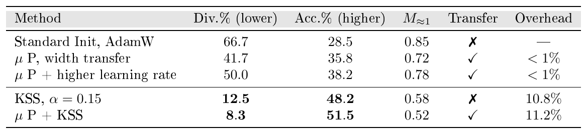
We extend the baseline comparisons to include $\mu$ P and the Layer-wise Adaptive Moments for Batch training (LAMB) optimizer ([52]).

$\mu$ P.

The $\mu$ P enables hyperparameter transfer across different model widths by appropriately scaling learning rates appropriately. Table 13 summarizes the $\mu$ P comparisons and the combined $\mu$ P + KSS setting. We observe moderate stability gains from $\mu$ P, with a 38\

::: {caption="Table 13: Comparison of mu P, standard parameterization, and KSS. Results use the No-Norm setting with learning rate ranges from 0.005 to 0.01 across 24 trials. Measured on the associative-recall task."}

:::

LAMB Optimizer.

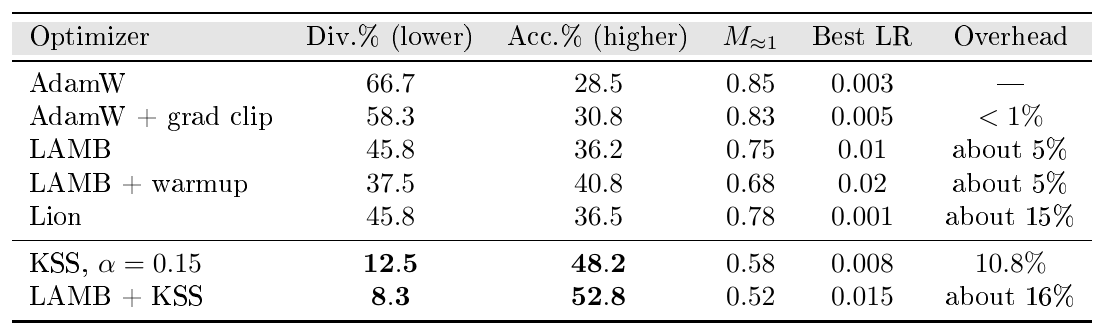
LAMB normalizes updates per layer, which changes spectral dynamics. Table 14 reports the optimizer comparison, including LAMB and Lion. LAMB outperforms AdamW: its layer-wise normalization provides implicit stability with a 31\

::: {caption="Table 14: Optimizer comparison among AdamW, LAMB, and Lion. Results use the No-Norm setting, 24 trials each. Measured on the associative-recall task."}

:::

G. Large-Scale Pretrained Model Analysis

GPT-2 Analysis.

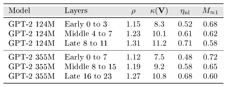
Table 15 reports layer-group spectral statistics for GPT-2 ([29]), and Figure 4 reveals a universal pattern. The normalized linear-fit error $\eta_{\mathrm{nl}}$ increases with depth, rising from $[0.48, 0.52]$ in the early layers to $[0.68, 0.71]$ in late layers. Simultaneously, the near-unit mass decreases from $M_{\approx 1} \in [0.68, 0.72]$ to $M_{\approx 1} \in [0.58, 0.60]$. This depth-wise trend has a clear implication: early layers are more linearly approximable, making DMD features more reliable, whereas late layers are less so.

::: {caption="Table 15: GPT-2 layer-wise spectral analysis. Start Linear, End Nonlinear pattern, shorthand for increasing $η_nl$. Spectral statistics are computed from residual-stream activations on a fixed set of short prompt sentences. Measured on a fixed short-prompt set."}

:::

H. Calibration

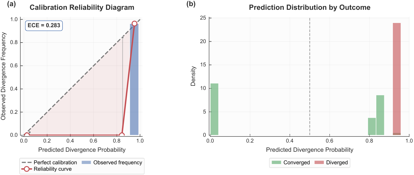
Beyond discrimination measured by AUROC, we assess calibration quality. Figure 5 shows that the risk score $M_{\approx 1}$ achieves an Expected Calibration Error (ECE) of 0.283, indicating moderate calibration. The reliability diagram reveals deviations between predicted probabilities and observed frequencies, while the distribution plots show clear separation between converged runs with lower $M_{\approx 1}$, corresponding to lower risk, and diverged runs with higher $M_{\approx 1}$, corresponding to higher risk. This calibration quality matters for deployment: practitioners can interpret RKSP's probability estimates for early termination decisions while accounting for the moderate calibration.

I. Novel Architecture Case Studies

To demonstrate RKSP's value beyond standard transformers, we analyze three emerging architectures: MoE ([42]), SSMs including Mamba ([43]), and KAN ([44]).

MoE Transformers

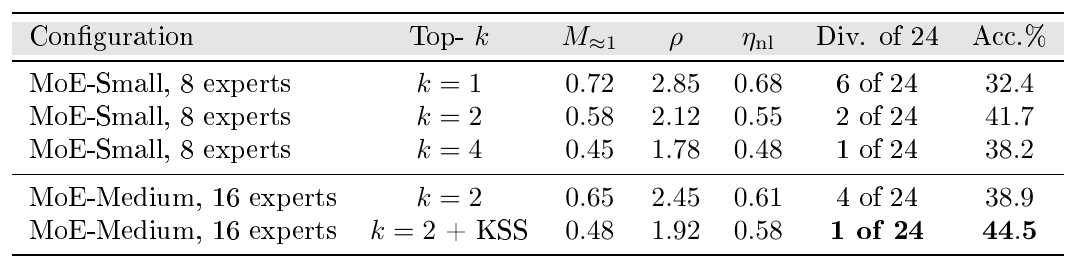
Table 16 presents a comparison of MoE routing and stability ([42]). MoE routing induces a higher normalized linear-fit error: $\eta_{\mathrm{nl}}$ increases 15\

::: {caption="Table 16: MoE transformer with RKSP analysis. Routing instability revealed via spectral signatures. Results use d=256, L=6, and 24 trials. Load balancing loss lambda=0.01. Measured on the synthetic LM task with random-token next-token prediction."}

:::

State Space Models: Mamba

Table 17 compares SSM and transformer spectral properties for Mamba ([43]). The theoretical explanation is straightforward: SSMs are designed with stable discrete-time dynamics via highly structured polynomial projection operator initialization. RKSP reveals this design choice explicitly in the spectral signature: Mamba exhibited $M_{<1} \approx 0.85 \gg M_{\approx 1} \approx 0.12$. This separation indicates strongly contractive dynamics with short memory and weak near-isometry; stability here comes from suppressed unstable modes in a highly contractive regime. In transformer regimes that are closer to near-normal, larger $M_{\approx 1}$ corresponds to weaker damping, longer-range signal retention, and higher instability risk.

::: {caption="Table 17: Mamba with RKSP analysis. Inherently stable spectral structure. Results use L=6, 24 trials. Measured on the synthetic LM task with random-token next-token prediction."}

:::

KAN

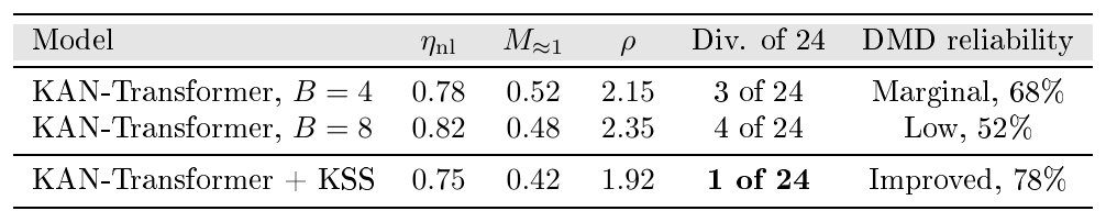
Table 18 reports KAN spectral diagnostics and KSS outcomes ([44]). KAN shows high normalized linear-fit error: B-spline basis functions produce $\eta_{\mathrm{nl}} \approx [0.78, 0.82]$, higher than the typical transformer layers with $[0.4, 0.7]$. Despite this high $\eta_{\mathrm{nl}}$, RKSP remains informative—ResDMD filtering enables spectral analysis for 68\

::: {caption="Table 18: KAN transformer with RKSP analysis. The B-spline nonlinearity challenges linear approximation. The B-spline order is B. We use d=256, L=6, and 24 trials. Measured on the synthetic LM task with random-token next-token prediction."}

:::

Cross-Architecture Summary

Table 11 summarizes cross-architecture metrics, while Figure 6 provides a normalized radar-chart view of the same comparison.

J. Practical Notes

RKSP and KSS are most valuable in three scenarios. First, when mechanistic understanding matters, RKSP explains why Pre-LN outperforms Post-LN through spectral signatures. Second, when pushing training limits, KSS enables learning rates that are 50% to 150% higher for faster convergence. Third, when deploying novel architectures, RKSP verifies stability before expensive training runs. Edge cases benefit most from these diagnostics—situations where standard normalization fails or where training operates near stability boundaries.

Fixup and ReZero-style identity initialization.

A common stabilization trick in deep residual networks and transformers is to initialize the final projection of each residual branch to zero, for example the attention and MLP output weights, so that the network starts close to an identity map ([22, 23]). In our notation, this yields a residual-off regime with a vanishing layer update $\mathbf{h}{\ell+1}-\mathbf{h}\ell \approx \mathbf{0}$, so the snapshot pairs satisfy $\mathbf{Y}\ell \approx \mathbf{X}\ell$ and DMD returns $\hat{\mathbf{A}}\ell \approx \mathbf{I}$. Consequently, $M{\approx 1}^\ell$ can be close to $1$ across layers even though training is often stable under Fixup and ReZero at initialization.

Taken alone, a near-identity spectrum might seem to imply maximal instability risk. However, our instability mechanism assumes two conditions: weak damping with large $M_{\approx 1}$ under near-normality, and non-degenerate layer-wise dynamics with appreciable updates so that perturbations and optimization noise are repeatedly injected and propagated across depth. Fixup and ReZero violate the second condition at initialization. When $\left|\tilde{\mathbf{Y}}\ell-\tilde{\mathbf{X}}\ell\right|_F$ is near zero, there is essentially no layer-wise update to analyze, and the resulting DMD spectrum is not informative about the noisy training-time regime we target.

Practically, this degeneracy is detectable from the same quantities RKSP already computes. When $\left|\tilde{\mathbf{Y}}\ell-\tilde{\mathbf{X}}\ell\right|F \approx 0$, the normalization in the nonlinearity becomes ill-conditioned, so $\eta{\mathrm{nl}}(\ell)$ should be interpreted as a DMD reliability flag rather than as a meaningful nonlinearity estimate. For Fixup and ReZero, RKSP becomes informative after a small amount of training, once the zero-initialized residual projections move away from zero and layer-wise updates become observable; at that point, RKSP can again capture whether the residual stream exhibits excessive near-isometric propagation (large $M_{\approx 1}$) that correlates with high-learning-rate divergence.

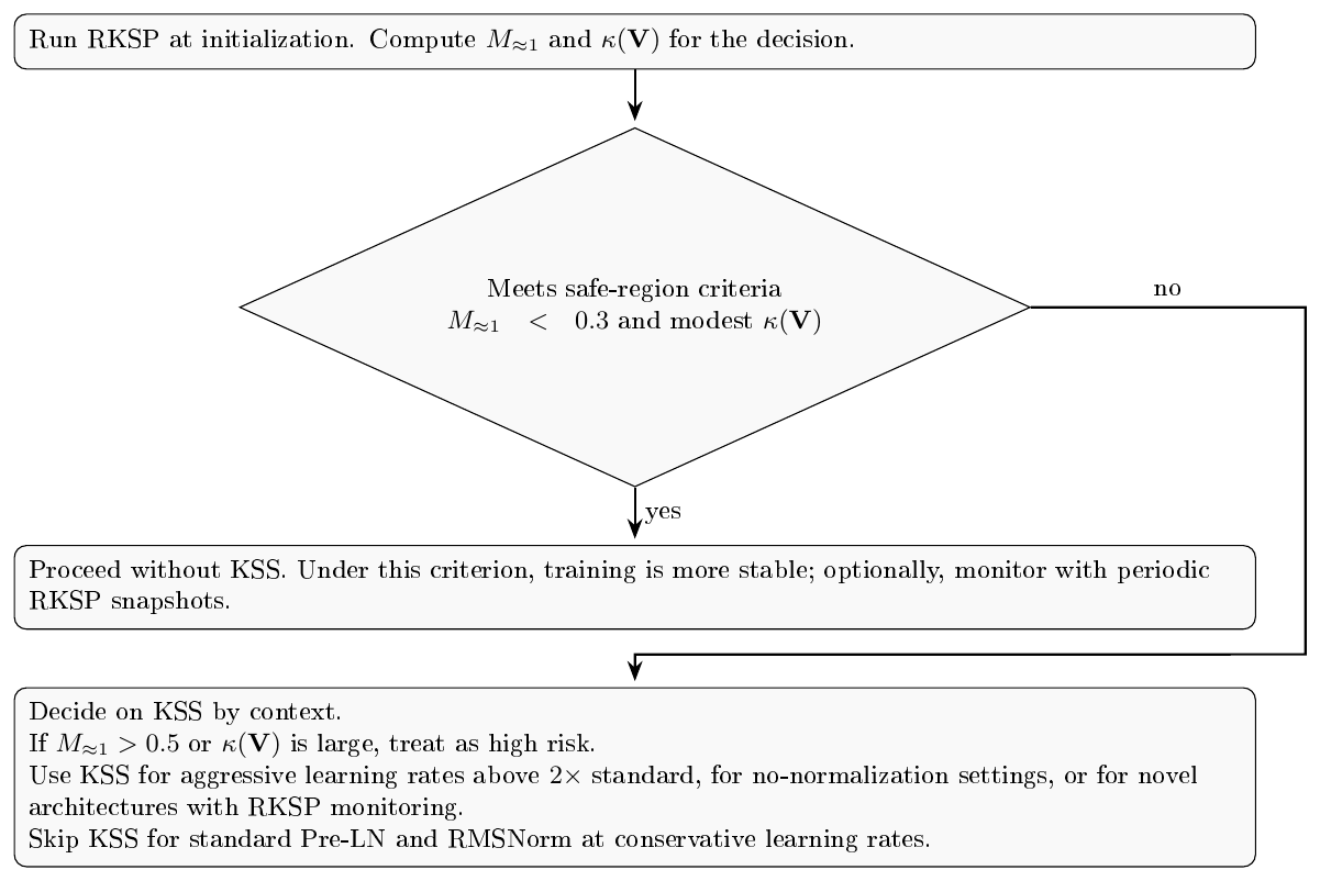
Practical deployment is straightforward. We recommend using RKSP in four scenarios: first, as a fast filter during architecture search; second, before expensive hyperparameter grid search; third, for periodic spectral monitoring during training; and fourth, for debugging checkpoints before divergence. Figure 7 provides an actionable decision process.

References

Section Summary: The references section compiles a list of academic papers and books that underpin the document’s discussion of neural network design and dynamical systems modeling. Many entries focus on transformer architectures, attention mechanisms, normalization methods, and residual connections, alongside foundational and applied work on dynamic mode decomposition and Koopman operators. The remaining citations address related topics such as optimization techniques, state-space models, and theoretical analyses of deep network training.

[1] Ashish Vaswani et al. (2017). Attention is All you Need. In NIPS. pp. 5998–6008.

[2] Lei Jimmy Ba et al. (2016). Layer Normalization. CoRR. abs/1607.06450.

[3] Razvan Pascanu et al. (2013). On the difficulty of training recurrent neural networks. In ICML (3). pp. 1310–1318.

[4] Tu, Jonathan H (2013). Dynamic mode decomposition: Theory and applications.

[5] Kaiming He et al. (2016). Deep Residual Learning for Image Recognition. In CVPR. pp. 770–778.

[6] Eldad Haber and Lars Ruthotto (2017). Stable Architectures for Deep Neural Networks. CoRR. abs/1705.03341.

[7] Tian Qi Chen et al. (2018). Neural Ordinary Differential Equations. In NeurIPS. pp. 6572–6583.

[8] Koopman, Bernard O (1931). Hamiltonian systems and transformation in Hilbert space. Proceedings of the National Academy of Sciences. 17(5). pp. 315–318.

[9] Mezić, Igor (2005). Spectral properties of dynamical systems, model reduction and decompositions. Nonlinear Dynamics. 41(1). pp. 309–325.

[10] Mezić, Igor (2013). Analysis of fluid flows via spectral properties of the Koopman operator. Annual review of fluid mechanics. 45(1). pp. 357–378.

[11] Rowley et al. (2009). Spectral analysis of nonlinear flows. Journal of fluid mechanics. 641. pp. 115–127.

[12] Schmid, Peter J (2010). Dynamic mode decomposition of numerical and experimental data. Journal of Fluid Mechanics. 656. pp. 5–28.

[13] J. Nathan Kutz et al. (2016). Dynamic mode decomposition - data-driven modeling of complex systems.

[14] Bethany Lusch et al. (2017). Deep learning for universal linear embeddings of nonlinear dynamics. CoRR. abs/1712.09707.

[15] Matthew O. Williams et al. (2015). A Data-Driven Approximation of the Koopman Operator: Extending Dynamic Mode Decomposition. J. Nonlinear Sci.. 25(6). pp. 1307–1346.

[16] Milan Korda and Igor Mezic (2018). Linear predictors for nonlinear dynamical systems: Koopman operator meets model predictive control. Autom.. 93. pp. 149–160.

[17] Samuel S. Schoenholz et al. (2017). Deep Information Propagation. In ICLR.

[18] Ben Poole et al. (2016). Exponential expressivity in deep neural networks through transient chaos. In NIPS. pp. 3360–3368.

[19] Jeffrey Pennington et al. (2017). Resurrecting the sigmoid in deep learning through dynamical isometry: theory and practice. In NIPS. pp. 4785–4795.

[20] Arthur Jacot et al. (2018). Neural Tangent Kernel: Convergence and Generalization in Neural Networks. In NeurIPS. pp. 8580–8589.

[21] Greg Yang et al. (2022). Tensor Programs V: Tuning Large Neural Networks via Zero-Shot Hyperparameter Transfer. CoRR. abs/2203.03466.

[22] Hongyi Zhang et al. (2019). Fixup Initialization: Residual Learning Without Normalization. In ICLR.

[23] Thomas Bachlechner et al. (2021). ReZero is all you need: fast convergence at large depth. In UAI. pp. 1352–1361.

[24] Andy Brock et al. (2021). High-Performance Large-Scale Image Recognition Without Normalization. In ICML. pp. 1059–1071.

[25] Kessy et al. (2018). Optimal whitening and decorrelation. The American Statistician. 72(4). pp. 309–314.

[26] Matthew J. Colbrook et al. (2022). Residual Dynamic Mode Decomposition: Robust and verified Koopmanism. CoRR. abs/2205.09779.

[27] N. Benjamin Erichson et al. (2019). Randomized Dynamic Mode Decomposition. SIAM J. Appl. Dyn. Syst.. 18(4). pp. 1867–1891.

[28] Trefethen, Lloyd N and Embree, Mark (2020). Spectra and pseudospectra: the behavior of nonnormal matrices and operators.

[29] Radford et al. (2019). Language models are unsupervised multitask learners. OpenAI blog. 1(8). pp. 9.

[30] Biao Zhang and Rico Sennrich (2019). Root Mean Square Layer Normalization. In NeurIPS. pp. 12360–12371.

[31] Hongyu Wang et al. (2024). DeepNet: Scaling Transformers to 1,000 Layers. IEEE Trans. Pattern Anal. Mach. Intell.. 46(10). pp. 6761–6774.

[32] Ruibin Xiong et al. (2020). On Layer Normalization in the Transformer Architecture. In ICML. pp. 10524–10533.

[33] Stephen Merity et al. (2017). Pointer Sentinel Mixture Models. In ICLR.

[34] Aaron Gokaslan and Vanya Cohen (2019). OpenWebText Corpus. http://Skylion007.github.io/OpenWebTextCorpus.

[35] Alexey Dosovitskiy et al. (2021). An Image is Worth 16x16 Words: Transformers for Image Recognition at Scale. In ICLR.

[36] Krizhevsky et al. (2009). Learning multiple layers of features from tiny images.

[37] Takeru Miyato et al. (2018). Spectral Normalization for Generative Adversarial Networks. In ICLR.

[38] Tim Salimans and Diederik P. Kingma (2016). Weight Normalization: A Simple Reparameterization to Accelerate Training of Deep Neural Networks. In NIPS. pp. 901.

[39] Pierre Foret et al. (2021). Sharpness-aware Minimization for Efficiently Improving Generalization. In ICLR.

[40] Xiangning Chen et al. (2023). Symbolic Discovery of Optimization Algorithms.

[41] Hugo Touvron et al. (2023). Llama 2: Open Foundation and Fine-Tuned Chat Models. CoRR. abs/2307.09288.

[42] Noam Shazeer et al. (2017). Outrageously Large Neural Networks: The Sparsely-Gated Mixture-of-Experts Layer. In ICLR.

[43] Albert Gu and Tri Dao (2023). Mamba: Linear-Time Sequence Modeling with Selective State Spaces. CoRR. abs/2312.00752.

[44] Ziming Liu et al. (2024). KAN: Kolmogorov-Arnold Networks. CoRR. abs/2404.19756.

[45] Joel A. Tropp (2012). User-Friendly Tail Bounds for Sums of Random Matrices. Found. Comput. Math.. 12(4). pp. 389–434.

[46] Nicholas J. Higham (2008). Functions of matrices - theory and computation.

[47] Kreiss, Heinz-Otto (1962). Über die Stabilitätsdefinition für Differenzengleichungen die partielle Differentialgleichungen approximieren. BIT Numerical Mathematics. 2(3). pp. 153–181.

[48] Daniel Y. Fu et al. (2023). Hungry Hungry Hippos: Towards Language Modeling with State Space Models. In ICLR.

[49] Simran Arora et al. (2024). Zoology: Measuring and Improving Recall in Efficient Language Models. In ICLR.

[50] Tom B. Brown et al. (2020). Language Models are Few-Shot Learners. In NeurIPS.

[51] Elhage et al. (2021). A mathematical framework for transformer circuits. Transformer Circuits Thread. 1(1). pp. 12.

[52] Yang You et al. (2020). Large Batch Optimization for Deep Learning: Training BERT in 76 minutes.