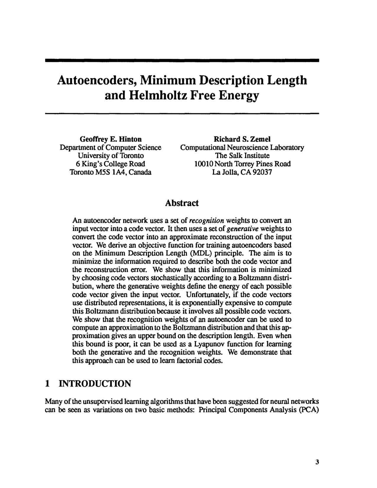
Autoencoders, Minimum Description Length and Helmholtz Free Energy

article1993NeurIPS1,528 citations

Establishes a theoretical framework connecting autoencoder training to Helmholtz free energy and Minimum Description Length, introducing the bits-back coding argument to efficiently learn non-linear, distributed factorial representations.

Listen

Modern data analysis relies heavily on unsupervised learning to discover underlying structure in complex, high-dimensional data without human labeling. Traditional methods force an unfavorable trade-off: techniques like Principal Components Analysis offer distributed, efficient representations but remain restricted to linear relationships, while Vector Quantization captures non-linear features but relies on purely localized, rigid code categories. Combining the strengths of both approaches has historically been intractable because evaluating distributed, non-linear codes requires calculating an exponentially large number of possible feature combinations.

The article establishes a practical training framework for autoencoder neural networks by applying the Minimum Description Length principle—which views optimal learning as compressing data to its shortest transmission length—and drawing an equivalence to Helmholtz free energy in statistical physics. Its main objective is to demonstrate that an autoencoder can efficiently learn non-linear, distributed factorial codes by approximating otherwise intractable probability distributions.

To evaluate this framework, the authors developed Factorial Vector Quantization, an approach where multiple sub-pools of hidden units independently and stochastically select features to reconstruct an input. Instead of running slow, approximate Monte Carlo simulations to calculate error derivatives, the authors derived a fast, exact calculation method for networks utilizing linear output units. The model was tested on an experimental benchmark dataset comprising 200 synthetic 8x12 pixel images depicting smooth spline curves with varying vertical control points.

The experimental findings show that the proposed factorial approach significantly outperforms standard models in compact data representation. The Factorial Vector Quantization network achieved an overall description length of approximately 25 bits per image (18 bits for reconstruction error and 7 bits for the code). In comparison, a standard stochastic vector quantizer with an identical total unit count required 40 total bits (36 bits for reconstruction and 4 bits for code), performing significantly worse at capturing image details. Training independent vector quantizers on separate vertical image slices required about 5 additional bits because they failed to smoothly blend curve segments. Additionally, while standard linear Principal Components Analysis marginally lowered reconstruction error, it resulted in a substantially higher code cost, making it far less compact overall.

These results demonstrate that autoencoders can bypass the computational bottleneck of distributed generative models. By treating the network's recognition weights as a tool to compute a tractable, factored approximation of true data distributions, the model creates an upper bound on description length that guarantees stable learning. This substantially improves performance and efficiency for unsupervised feature extraction, allowing complex data representations to be learned without exponential processing overhead.

Based on these findings, teams developing unsupervised generative models should consider adopting Helmholtz free energy and Minimum Description Length bounds as optimization objectives to balance code efficiency and reconstruction accuracy. Prior to scaling this framework to broader enterprise domains, technical leaders should initiate pilot studies across more complex and higher-dimensional datasets. Further development is also warranted to explore alternative configurations, such as population codes and deeper network architectures.

The conclusions of the article are subject to specific boundary conditions. The demonstrations rely on a controlled synthetic image dataset and assume linear output units with Gaussian reconstruction error to compute exact gradient values. In addition, the framework purposefully ignores the one-time cost of communicating network model parameters by assuming large data volumes. Despite these simplifying assumptions, there is high confidence in the foundational theoretical framework and its capacity to discover compact, non-linear representations across unsupervised learning domains.

Computational Neuroscience Laboratory Salk Institute for Biological Studies University of Toronto code vectors helmholtz lyapunov autoencoders minimum description length Helmholtz free energy

Hinton et al (1993).pdf

Paper: Keeping Neural Networks Simple by Minimizing the Description Length of the Weights, Geoffrey E. Hinton et al. (1993). It introduces the Minimum Description Length (MDL) and variational coding framework for neural network weights that directly underpins the source's free-energy formulation for autoencoders.
Paper: A Learning Algorithm for Boltzmann Machines, David H. Ackley et al. (1985). It introduces Boltzmann distributions and energy-based representations in neural networks, which the source relies on for formulating stochastic code vectors and Helmholtz free energy.
Paper: A Simple Weight Decay Can Improve Generalization, Anders Krogh et al. (1991). It provides the classic theoretical analysis of weight penalization and capacity control that motivates information-theoretic regularization in autoencoders.

Paper: An Introduction to Variational Autoencoders, Diederik P. Kingma et al. (2019). It synthesizes modern amortized variational inference and autoencoding, which directly evolved from the recognition-generative variational free energy framework introduced in the source.
Paper: Stochastic Backpropagation and Approximate Inference in Deep Generative Models, Danilo Jimenez Rezende et al. (2014). It builds upon the recognition-generative autoencoder paradigm by introducing stochastic backpropagation to optimize deep variational lower bounds.
Paper: A Fast Learning Algorithm for Deep Belief Nets, Geoffrey E. Hinton et al. (2006). It advances the source's ideas of learning hierarchical generative models and complementary representations using layer-wise generative and recognition components.
Paper: Tutorial on Variational Autoencoders, Carl Doersch (2016). It provides a clear modern tutorial on variational autoencoders, explaining how latent free energy bounds are implemented and trained in deep neural networks.
Paper: Practical Variational Inference for Neural Networks, Alex Graves (2011). It applies the Minimum Description Length and variational free-energy principles from the source to modern gradient-based neural network training.
Paper: Importance Weighted Autoencoders, Yuri Burda et al. (2016). It generalizes variational autoencoder objectives to tighter lower bounds using importance weighting, directly extending variational code approximation techniques.
Paper: Fixing a Broken ELBO, Alexander A. Alemi et al. (2018). It critically analyzes the rate-distortion and mutual information properties of variational autoencoders derived from the evidence lower bound.
Paper: Variational Lossy Autoencoder, Xi Chen et al. (2017). It extends variational autoencoding using an explicit bits-back coding and information-theoretic perspective to control lossy code representations.
Paper: Stacked Denoising Autoencoders: Learning Useful Representations in a Deep Network with a Local Denoising Criterion, Pascal Vincent et al. (2010). It extends representation learning in autoencoders by introducing deep stacking and denoising objectives to extract robust hierarchical features.
Paper: Representation Learning: A Review and New Perspectives, Yoshua Bengio et al. (2012). It provides a comprehensive retrospective on representation learning, placing autoencoders, Boltzmann machines, and disentangled factorial codes into modern perspective.

Cover for Autoencoders, Minimum Description Length and Helmholtz Free Energy

Abstract

An autoencoder network uses a set of recognition weights to convert an input vector into a code vector. It then uses a set of generative weights to convert the code vector into an approximate reconstruction of the input vector. We derive an objective function for training autoencoders based on the Minimum Description Length (MDL) principle. The aim is to minimize the information required to describe both the code vector and the reconstruction error. We show that this information is minimized by choosing code vectors stochastically according to a Boltzmann distribution, where the generative weights define the energy of each possible code vector given the input vector. Unfortunately, if the code vectors use distributed representations, it is exponentially expensive to compute this Boltzmann distribution because it involves all possible code vectors. We show that the recognition weights of an autoencoder can be used to compute an approximation to the Boltzmann distribution and that this approximation gives an upper bound on the description length. Even when this bound is poor, it can be used as a Lyapunov function for learning both the generative and the recognition weights. We demonstrate that this approach can be used to learn factorial codes.

Topics

code vectors helmholtz lyapunov reconstruction auto encoders variational autoencoders

Keywords

autoencoders minimum description length Helmholtz free energy vector quantization generative models stochastic complexity EM algorithm Boltzmann distribution factorial codes unsupervised learning

1 INTRODUCTION
2 THE MINIMUM DESCRIPTION LENGTH APPROACH
2.1 The "bits-back" argument
3 FACTORIAL STOCHASTIC VECTOR QUANTIZATION
3.1 Computing the Expected Reconstruction Error
4 AN EXAMPLE OF FACTORIAL VECTOR QUANTIZATION
5 DISCUSSION
Acknowledgements
References

Knowls

Knowl 1 — Bits-Back Coding and Helmholtz Free Energy Objective for Autoencoders
model/method
Under the Minimum Description Length (MDL) communication framework for autoencoders, communicating an input vector $x \in \mathbb{R}^k$ using a discrete latent code $i$ incurs a code cost determined by its prior probability $\pi_i$ and a reconstruction error cost under an assumed zero-mean Gaussian distribution with variance $\sigma^2$ and quantization width $t$ . The energy (description length using code $i$ ) is:

$E_i = -\log \pi_i - k \log t + \frac{k}{2}\log(2\pi \sigma^2) + \frac{d_i^2}{2\sigma^2}$

where $d_i^2 = \|x - \hat{x}_i\|^2$ is the squared Euclidean reconstruction error.

When the sender chooses code $i$ stochastically according to a probability distribution $p_i$ , the sender can use this stochastic choice to transmit auxiliary information at zero extra cost (the "bits-back" principle). Once the receiver decodes $x$ , they run the same recognition procedure to recover the distribution $p$ , saving $H(p) = -\sum_i p_i \log p_i$ bits. The net expected description length is the Helmholtz free energy:

$F = \sum_i p_i E_i - H(p) = \sum_i p_i E_i + \sum_i p_i \log p_i$

The optimal distribution minimizing $F$ is the Boltzmann distribution (the exact posterior under the generative model):

$p_i = \frac{e^{-E_i}}{\sum_j e^{-E_j}}$
Knowl 2 — Variational Free Energy Upper Bound and Lyapunov Optimization
theoretical result
When an exact posterior distribution $p_i = \frac{e^{-E_i}}{\sum_j e^{-E_j}}$ over $m^d$ distributed latent codes is computationally intractable, any tractable suboptimal distribution $q$ parameterized by a feed-forward recognition network can be substituted. The resulting non-equilibrium Helmholtz free energy,

$F(q, \theta) = \sum_i q_i E_i(\theta) + \sum_i q_i \log q_i$

where $\theta$ represents the generative parameters defining code energies $E_i(\theta)$ , is a rigorous upper bound on the true optimal description length $-\log \sum_i e^{-E_i(\theta)}$ .

The gap between $F(q, \theta)$ and the optimal description length is the Kullback–Leibler divergence $D_{\mathrm{KL}}(q \parallel p)$ . Therefore, $F(q, \theta)$ acts as a Lyapunov function for simultaneous gradient optimization:
1. Gradients with respect to recognition weights minimize $D_{\mathrm{KL}}(q \parallel p)$ , driving the approximate distribution $q$ toward the true generative posterior $p$ .
2. Gradients with respect to generative weights $\theta$ minimize expected reconstruction and prior costs under $q$ , while simultaneously encouraging generative weights toward configurations where the true posterior is well-approximated by the family of $q$ .
Learning remains valid and monotonic without requiring the recognition model to reach thermal equilibrium before updating generative parameters.
Knowl 3 — Factorial Stochastic Vector Quantization Architecture
model/method
Factorial Stochastic Vector Quantization (FSVQ) represents inputs using a distributed code structured into $d$ separate pools of hidden units, with each pool $v \in \{1, \dots, d\}$ containing $m$ mutually exclusive (winner-take-all) units. The total number of composite distributed states is $m^d$ .

To ensure computational tractability, the joint distribution over all $m^d$ states is approximated by a factorial distribution factored across the $d$ pools:

$q(i_1, \dots, i_d) = \prod_{v=1}^d h_{i_v}^v$

where $h_i^v$ is the activation probability of unit $i \in \{1, \dots, m\}$ in pool $v$ , satisfying $\sum_{i=1}^m h_i^v = 1$ for each $v$ . These activation probabilities are computed deterministically from the input vector by a non-stochastic feed-forward recognition network.
Knowl 4 — Exact Expected Reconstruction Error and Output Variance for Linear Decoders
equation
For a Factorial Stochastic Vector Quantizer with linear output units and squared reconstruction error, exact gradients of the expected reconstruction cost can be computed without Monte Carlo sampling. Let $h_i^v$ denote the selection probability of unit $i \in \{1, \dots, m\}$ in pool $v \in \{1, \dots, d\}$ , $w_{ji}^v$ be the generative weight from unit $i$ of pool $v$ to output unit $j$ , and $b_j$ be the output bias of unit $j$ .

The expected reconstructed output $y_j = \mathbb{E}[y_j^{\text{stoch}}]$ for unit $j$ is:

$y_j = b_j + \sum_{v=1}^d \sum_{i=1}^m w_{ji}^v h_i^v$

Assuming stochastic selections across different pools are independent, the output variance $V_j = \mathrm{Var}(y_j^{\text{stoch}})$ contributed by the stochastic choices within pools is:

$V_j = \sum_{v=1}^d \sum_{i=1}^m h_i^v \left(w_{ji}^v - \sum_{k=1}^m w_{jk}^v h_k^v\right)^2$

For a target value $d_j$ , the total expected squared reconstruction error for output unit $j$ is:

$\mathbb{E}\left[(y_j^{\text{stoch}} - d_j)^2\right] = V_j + (y_j - d_j)^2$

This closed form allows analytic backpropagation through the free energy objective with respect to both recognition and generative parameters.
Knowl 5 — Factorial Representation Learning on Blurred Spline Images
empirical result
Factorial Stochastic Vector Quantization (FSVQ) was evaluated on a dataset of 200 synthetic $8 \times 12$ pixel images generated by fitting splines to 5 control points with randomly chosen vertical positions and fixed horizontal positions, followed by Gaussian blurring (5 underlying degrees of freedom).

An FSVQ network configured with $d = 4$ pools of $m = 6$ units (24 hidden units total) learned to dedicate each pool to the vertical position and local shape of one of the 4 spline segments connecting consecutive control points. On unseen test images generated from the same process:
- Factorial VQ (4 pools of 6 units) achieved a reconstruction cost of $\approx 18$ bits and a code cost of $\approx 7$ bits (total $\approx 25$ bits).
- Standard stochastic VQ (single pool of 24 units) achieved a reconstruction cost of $36$ bits and a code cost of $4$ bits (total $40$ bits).
- Four separate stochastic VQs trained on independent $8 \times 3$ vertical image slices achieved a description length $\approx 5$ bits worse than FSVQ ( $\\approx 30$ bits total) due to inability to smoothly blend spline boundaries across slices.
- Linear autoencoder (PCA with 24 units) achieved slightly lower reconstruction error than FSVQ but required a substantially higher code cost.

Coverage note — No substantial contributed material was omitted. General conceptual discussions of population codes and standard PCA/mixture-of-Gaussians models were omitted as background context.

References

1.Baldi, P. and Hornik, K. (1989) Neural networks and principal components analysis: Learning from examples without local minima. Neural Networks, 2, 53-58.
2.Galland, C. C. (1993) The limitations of deterministic Boltzmann machine learning. Network, 4, 355-379.
3.Hinton, G. E. (1989) Connectionist learning procedures. Artificial Intelligence, 40, 185-234.
4.Neal, R., and Hinton, G. E. (1993) A new view of the EM algorithm that justifies incremental and other variants. Manuscript available from the authors.
5.Rissanen, J. ( 1989) Stochastic Complexity in Statistical Inquiry. World Scientific Publishing Co., Singapore.
6.Zemel, R. S. (1993) A Minimum Description Length Framework for Unsupervised Learning. PhD. Thesis, Department of Computer Science, University of Toronto.
7.Zemel, R. S. and Hinton, G. E. (1994) Developing Population Codes by Minimizing Description Length. In J. Cowan, G. Tesauro, and J. Alspector (Eds.), Advances in Neural Information Processing Systems 6, San Mateo, CA: Morgan Kaufmann.

Citation

MLA

Hinton, G. E., and R. Zemel. “Autoencoders, Minimum Description Length and Helmholtz Free Energy”. Advances in Neural Information Processing Systems, vol. 6, 1993, https://proceedings.neurips.cc/paper_files/paper/1993/file/9e3cfc48eccf81a0d57663e129aef3cb-Paper.pdf.

APA

Hinton, G. E., & Zemel, R. (1993). Autoencoders, Minimum Description Length and Helmholtz Free Energy. Advances in Neural Information Processing Systems, 6. https://proceedings.neurips.cc/paper_files/paper/1993/file/9e3cfc48eccf81a0d57663e129aef3cb-Paper.pdf

Chicago

Hinton, G. E., and R. Zemel. 1993. “Autoencoders, Minimum Description Length and Helmholtz Free Energy”. Advances in Neural Information Processing Systems 6. https://proceedings.neurips.cc/paper_files/paper/1993/file/9e3cfc48eccf81a0d57663e129aef3cb-Paper.pdf.

Harvard

Hinton, G.E. and Zemel, R. (1993) “Autoencoders, Minimum Description Length and Helmholtz Free Energy”, Advances in Neural Information Processing Systems. Curran Associates, Inc. Available at: https://proceedings.neurips.cc/paper_files/paper/1993/file/9e3cfc48eccf81a0d57663e129aef3cb-Paper.pdf.

Vancouver

1. Hinton GE, Zemel R (1993) Autoencoders, Minimum Description Length and Helmholtz Free Energy. Advances in Neural Information Processing Systems 6:

BibTeX

@inproceedings{hinton1993autoencoders,
  title = {Autoencoders, Minimum Description Length and Helmholtz Free Energy},
  author = {Hinton, Geoffrey E. and Zemel, Richard},
  year = {1993},
  booktitle = {Advances in Neural Information Processing Systems},
  publisher = {Curran Associates, Inc.},
  volume = {6},
  url = {https://proceedings.neurips.cc/paper_files/paper/1993/file/9e3cfc48eccf81a0d57663e129aef3cb-Paper.pdf}
}

Metadata:DOI registry

Access the Paper

This paper is available from its original source. Click below to access the PDF.

Open PDF

License: Published with permission

Autoencoders, Minimum Description Length and Helmholtz Free Energy

Abstract

Topics

Keywords

Table of Contents

Knowls

Knowl 1 — Bits-Back Coding and Helmholtz Free Energy Objective for Autoencoders

Knowl 2 — Variational Free Energy Upper Bound and Lyapunov Optimization

Knowl 3 — Factorial Stochastic Vector Quantization Architecture

Knowl 4 — Exact Expected Reconstruction Error and Output Variance for Linear Decoders

Knowl 5 — Factorial Representation Learning on Blurred Spline Images

References

Citation

BibTeX

Access the Paper