Generalized Focal Loss: Learning Qualified and Distributed Bounding Boxes for Dense Object Detection

Abstract

One-stage detector basically formulates object detection as dense classification and localization (i.e., bounding box regression). The classification is usually optimized by Focal Loss and the box location is commonly learned under Dirac delta distribution. A recent trend for one-stage detectors is to introduce an individual prediction branch to estimate the quality of localization, where the predicted quality facilitates the classification to improve detection performance. This paper delves into the representations of the above three fundamental elements: quality estimation, classification and localization. Two problems are discovered in existing practices, including (1) the inconsistent usage of the quality estimation and classification between training and inference (i.e., separately trained but compositely used in test) and (2) the inflexible Dirac delta distribution for localization when there is ambiguity and uncertainty which is often the case in complex scenes. To address the problems, we design new representations for these elements. Specifically, we merge the quality estimation into the class prediction vector to form a joint representation of localization quality and classification, and use a vector to represent arbitrary distribution of box locations. The improved representations eliminate the inconsistency risk and accurately depict the flexible distribution in real data, but contain continuous labels, which is beyond the scope of Focal Loss. We then propose Generalized Focal Loss (GFL) that generalizes Focal Loss from its discrete form to the continuous version for successful optimization. On COCO test-dev, GFL achieves 45.0% AP using ResNet-101 backbone, surpassing state-of-the-art SAPD (43.5%) and ATSS (43.6%) with higher or comparable inference speed, under the same backbone and training settings. Notably, our best model can achieve a single-model single-scale AP of 48.2%, at 10 FPS on a single 2080Ti GPU. Code and pretrained models are available at https://github.com/implus/GFocal.

Executive Summary: Dense single-stage object detection systems in computer vision are widely used to identify and locate target objects in digital images. However, conventional detection pipelines suffer from two structural shortcomings. First, they train object classification and localization quality scores separately but multiply them together during final inference, which often causes background clutter or low-quality boxes to be mistakenly prioritized. Second, standard models represent bounding box boundaries as rigid, single-point coordinates, which fails to capture boundary ambiguity caused by occlusion, shadows, or visual blur.

The article set out to introduce and evaluate Generalized Focal Loss, a unified mathematical framework designed to bridge the gap between training and testing while modeling object boundaries as flexible, continuous probability distributions rather than fixed coordinates.

The authors designed two specialized loss functions—Quality Focal Loss, which merges category classification and localization quality into a single continuous variable, and Distribution Focal Loss, which learns arbitrary spatial probability distributions for object edges. To validate this framework, the authors conducted extensive experimental evaluations on the industry-standard Microsoft COCO detection benchmark using multiple widely used detector backbones and compared performance against leading state-of-the-art models.

The analysis yielded several key findings. First, integrating the proposed loss functions consistently improved accuracy across multiple standard detector architectures without adding computational overhead or slowing inference speeds. Second, on the COCO test benchmark, the method achieved a 45.0% average precision using a standard ResNet-101 backbone, outperforming leading existing detectors such as SAPD (43.5%) and ATSS (43.6%) under identical training configurations. Third, the enhanced configuration achieved a top-tier detection accuracy of 48.2% average precision while maintaining a practical processing speed of 10 frames per second on a single standard graphics processing unit.

These results demonstrate that aligning training targets directly with deployment scoring mechanisms eliminates ranking errors, while flexible boundary distributions provide critical robustness when dealing with complex or occluded visual scenes. For organizations deploying vision-based automation, robotics, or surveillance, this technique delivers higher detection reliability and precision with virtually no penalty to hardware costs, latency, or system complexity.

Based on these findings, technical teams should consider adopting the proposed joint classification-quality representation and continuous loss formulations as drop-in enhancements for dense detection systems. Organizations should evaluate these techniques in pilot pipelines to boost precision in challenging real-world environments. Future development should explore extending continuous distribution modeling to related computer vision tasks, including three-dimensional object detection and video tracking.

Confidence in these findings is high due to rigorous benchmarking across standard datasets and clear comparative baselines. A minor limitation is that the primary evaluations were conducted within standard 2D image benchmarks, meaning performance across highly specialized domains, such as medical scanning or aerial imaging, will require domain-specific validation and parameter calibration.

1. Introduction

Section Summary: Recent object detectors represent bounding boxes with simple fixed forms and predict classification scores separately from localization quality measures such as IoU, yet these choices produce mismatches between training and inference as well as unreliable quality estimates for background regions. The paper identifies that such separate handling allows negative samples to receive spuriously high quality scores and that rigid box models overlook boundary uncertainty and complex location distributions in real data. To close these gaps, the work proposes a single joint classification-and-quality output together with a flexible, distribution-based box representation that can be trained end-to-end and used directly at test time.

Recently, dense detectors have gradually led the trend of object detection, whilst the attention on the representation of bounding boxes and their localization quality estimation leads to the encouraging advancement. Specifically, bounding box representation is modeled as a simple Dirac delta distribution [1, 2, 3, 4, 5], which is widely used over past years. As popularized in FCOS [4], predicting an additional localization quality (e.g., IoU score [6] or centerness score [4]) brings consistent improvements of detection accuracy, when the quality estimation is combined (usually multiplied) with classification confidence as final scores [7, 8, 4, 6, 9] for the rank process of Non-Maximum Suppression (NMS) during inference. Despite their success, we observe the following problems in existing practices:

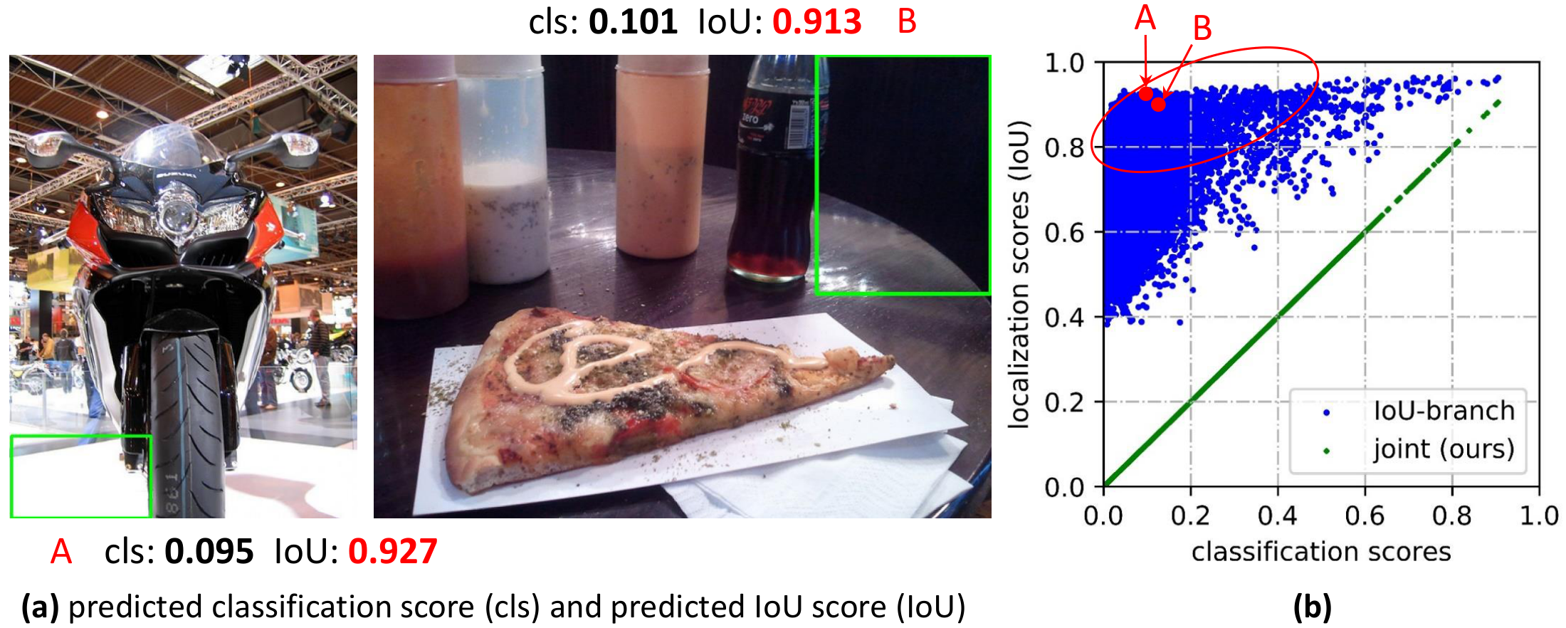
Inconsistent usage of localization quality estimation and classification score between training and inference: (1) In recent dense detectors, the localization quality estimation and classification score are usually trained independently but compositely utilized (e.g., multiplication) during inference [4, 6] (Figure 1(a)); (2) The supervision of the localization quality estimation is currently assigned for positive samples only [7, 8, 4, 6, 9], which is unreliable as negatives may get chances to have uncontrollably higher quality predictions (Figure 2(a)). These two factors result in a gap between training and test, and would potentially degrade the detection performance, e.g., negative instances with randomly high-quality scores could rank in front of positive examples with lower quality prediction during NMS.

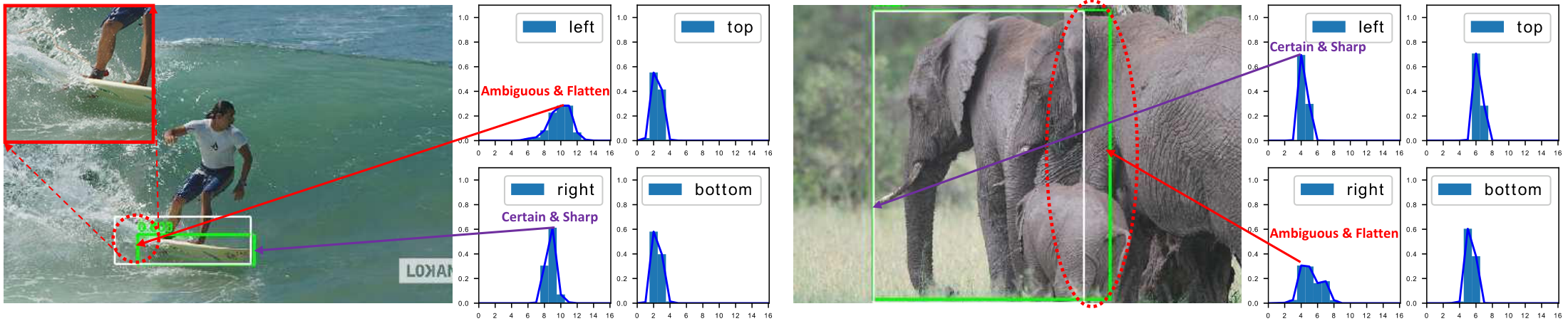
Inflexible representation of bounding boxes: The widely used bounding box representation can be viewed as Dirac delta distribution [10, 11, 12, 13, 2, 4, 14, 5] of the target box coordinates. However, it fails to consider the ambiguity and uncertainty in datasets (see the unclear boundaries of the figures in Figure 3). Although some recent works [1, 15] model boxes as Gaussian distributions, it is too simple to capture the real distribution of the locations of bounding boxes. In fact, the real distribution can be more arbitrary and flexible [1], without the necessity of being symmetric like the Gaussian function.

To address the above problems, we design new representations for the bounding boxes and their localization quality. For localization quality representation, we propose to merge it with the classification score into a single and unified representation: a classification vector where its value at the ground-truth category index refers to its corresponding localization quality (typically the IoU score between the predicted box and the corresponding ground-truth box in this paper). In this way, we unify classification score and IoU score into a joint and single variable (denoted as "classification-IoU joint representation"), which can be trained in an end-to-end fashion, whilst directly utilized during inference (Figure 1(b)). As a result, it eliminates the training-test inconsistency (Figure 1(b)) and enables the strongest correlation (Figure 2 (b)) between localization quality and classification. Further, the negatives will be supervised with 0 quality scores, thereby the overall quality predictions become more confidential and reliable. It is especially beneficial for dense object detectors as they rank all candidates regularly sampled across an entire image. For bounding box representation, we propose to represent the arbitrary distribution (denoted as "General distribution" in this paper) of box locations by directly learning the discretized probability distribution over its continuous space, without introducing any other stronger priors (e.g., Gaussian [1, 15]). Consequently, we can obtain more reliable and accurate bounding box estimations, whilst being aware of a variety of their underlying distributions (see the predicted distributions in Figure 3 and Supplementary Materials).

The improved representations then pose challenges for optimization. Traditionally for dense detectors, the classification branch is optimized with Focal Loss [2] (FL). FL can successfully handles the class imbalance problem via reshaping the standard cross entropy loss. However, for the case of the proposed classification-IoU joint representation, in addition to the imbalance risk that still exists, we face a new problem with continuous IoU label (0$\sim$1) as supervisions, as the original FL only supports discrete ${1, 0}$ category label currently. We successfully solve the problem by extending FL from ${1, 0}$ discrete version to its continuous variant, termed Generalized Focal Loss (GFL). Different from FL, GFL considers a much general case in which the globally optimized solution is able to target at any desired continuous value, rather than the discrete ones. More specifically in this paper, GFL can be specialized into Quality Focal Loss (QFL) and Distribution Focal Loss (DFL), for optimizing the improved two representations respectively: QFL focuses on a sparse set of hard examples and simultaneously produces their continuous 0$\sim$1 quality estimations on the corresponding category; DFL makes the network to rapidly focus on learning the probabilities of values around the continuous locations of target bounding boxes, under an arbitrary and flexible distribution.

We demonstrate three advantages of GFL: (1) It bridges the gap between training and test when one-stage detectors are facilitated with additional quality estimation, leading to a simpler, joint and effective representation of both classification and localization quality; (2) It well models the flexible underlying distribution for bounding boxes, which provides more informative and accurate box locations; (3) The performance of one-stage detectors can be consistently boosted without introducing additional overhead. On COCO test-dev, GFL achieves 45.0% AP with ResNet-101 backbone, surpassing state-of-the-art SAPD (43.5%) and ATSS (43.6%). Our best model can achieve a single-model single-scale AP of 48.2% whilst running at 10 FPS on a single 2080Ti GPU.

2. Related Work

Section Summary: Existing methods for estimating localization quality in object detection typically rely on a separate prediction branch to output scores such as IoU or centerness, which creates mismatches between training and testing and produces unreliable results. Other approaches attempt to link classification scores more closely to localization accuracy by adjusting loss weights, yet these adjustments remain indirect and do not alter the fundamental objectives of the classification loss. For representing bounding boxes, prior work has used either rigid Dirac delta distributions or simplified Gaussian assumptions to capture uncertainty, but both are viewed as inadequate for modeling the complex distributions found in real data.

Representation of localization quality. Existing practices like Fitness NMS [16], IoU-Net [7], MS R-CNN [8], FCOS [4] and IoU-aware [6] utilize a separate branch to perform localization quality estimation in a form of IoU or centerness score. As mentioned in Section 1, this separate formulation causes the inconsistency between training and test as well as unreliable quality predictions. Instead of introducing an additional branch, PISA [17] and IoU-balance [18] assign different weights in the classification loss based on their localization qualities, aiming at enhancing the correlation between the classification score and localization accuracy. However, the weight strategy is of implicit and limited benefits since it does not change the optimum of the loss objectives for classification.

Representation of bounding boxes. Dirac delta distribution [10, 11, 12, 13, 2, 4, 14, 5] governs the representation of bounding boxes over past years. Recently, Gaussian assumption [1, 15] is adopted to learn the uncertainty by introducing a predicted variance. Unfortunately, existing representations are either too rigid or too simplified, which can not reflect the complex underlying distribution in real data. In this paper, we further relax the assumption and directly learn the more arbitrary, flexible General distribution of bounding boxes, whilst being more informative and accurate.

3. Method

Section Summary: The section reviews the original Focal Loss for addressing extreme foreground-background imbalance in one-stage detectors, then introduces two extensions. Quality Focal Loss adapts the loss to continuous IoU-based targets so the classification branch can jointly predict both category and localization quality. Distribution Focal Loss models each bounding-box coordinate as a flexible distribution and concentrates learning on probabilities near the target value; both are combined into a unified Generalized Focal Loss framework.

In this section, we first review the original Focal Loss [2] (FL) for learning dense classification scores of one-stage detectors. Next, we present the details for the improved representations of localization quality estimation and bounding boxes, which are successfully optimized via the proposed Quality Focal Loss (QFL) and Distribution Focal Loss (DFL), respectively. Finally, we summarize the formulations of QFL and DFL into a unified perspective termed Generalized Focal Loss (GFL), as a flexible extension of FL, to facilitate further promotion and general understanding in the future.

Focal Loss (FL). The original FL [2] is proposed to address the one-stage object detection scenario where an extreme imbalance between foreground and background classes often exists during training. A typical form of FL is as follows (we ignore $\alpha_t$ in original paper [2] for simplicity):

$ \textbf{FL}(p) = - (1 - p_t)^\gamma\log(p_t), p_t = \left{\begin{array}{rc}p, & \text{when}\ \ y = 1 \1 - p, & \text{when}\ \ y = 0\end{array} \right. $

where $y \in {1, 0}$ specifies the ground-truth class and $p \in [0, 1]$ denotes the estimated probability for the class with label $y = 1$. $\gamma$ is the tunable focusing parameter. Specifically, FL consists of a standard cross entropy part $-\log(p_t)$ and a dynamically scaling factor part $(1 - p_t)^\gamma$, where the scaling factor $(1 - p_t)^\gamma$ automatically down-weights the contribution of easy examples during training and rapidly focuses the model on hard examples.

Quality Focal Loss (QFL). To solve the aforementioned inconsistency problem between training and test phases, we present a joint representation of localization quality (i.e., IoU score) and classification score ("classification-IoU" for short), where its supervision softens the standard one-hot category label and leads to a possible float target $y \in [0, 1]$ on the corresponding category (see the classification branch in Figure 4). Specifically, $y = 0$ denotes the negative samples with 0 quality score, and $0 < y \le 1$ stands for the positive samples with target IoU score $y$. Note that the localization quality label $y$ follows the conventional definition as in [6, 7]: IoU score between the predicted bounding box and its corresponding ground-truth bounding box during training, with a dynamic value being 0$\sim$1. Following [2, 4], we adopt the multiple binary classification with sigmoid operators $\sigma(\cdot)$ for multi-class implementation. For simplicity, the output of sigmoid is marked as $\sigma$.

Since the proposed classification-IoU joint representation requires dense supervisions over an entire image and the class imbalance problem still occurs, the idea of FL must be inherited. However, the current form of FL only supports ${1, 0}$ discrete labels, but our new labels contain decimals. Therefore, we propose to extend the two parts of FL for enabling the successful training under the case of joint representation: (1) The cross entropy part $-\log(p_t)$ is expanded into its complete version $-\big((1 - y)\log(1 - \sigma) + y\log(\sigma)\big)$; (2) The scaling factor part $(1 - p_t)^\gamma$ is generalized into the absolute distance between the estimation $\sigma$ and its continuous label $y$, i.e., $|y - \sigma|^\beta$ ($\beta \ge 0$), here $|\cdot|$ guarantees the non-negativity. Subsequently, we combine the above two extended parts to formulate the complete loss objective, which is termed as Quality Focal Loss (QFL):

$ \textbf{QFL}(\sigma) = -\big|y - \sigma\big|^{\beta}\big((1 - y)\log(1 - \sigma) + y\log(\sigma)\big). $

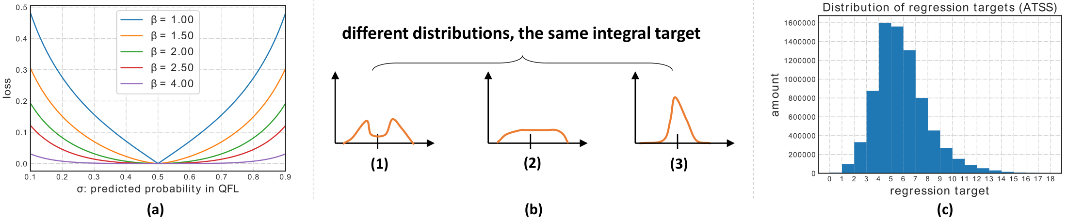
Note that $\sigma = y$ is the global minimum solution of QFL. QFL is visualized for several values of $\beta$ in Figure 5(a) under quality label $y = 0.5$. Similar to FL, the term $\big|y - \sigma\big|^{\beta}$ of QFL behaves as a modulating factor: when the quality estimation of an example is inaccurate and deviated away from label $y$, the modulating factor is relatively large, thus it pays more attention to learning this hard example. As the quality estimation becomes accurate, i.e., $\sigma \to y$, the factor goes to 0 and the loss for well-estimated examples is down-weighted, in which the parameter $\beta$ controls the down-weighting rate smoothly ($\beta = 2$ works best for QFL in our experiments).

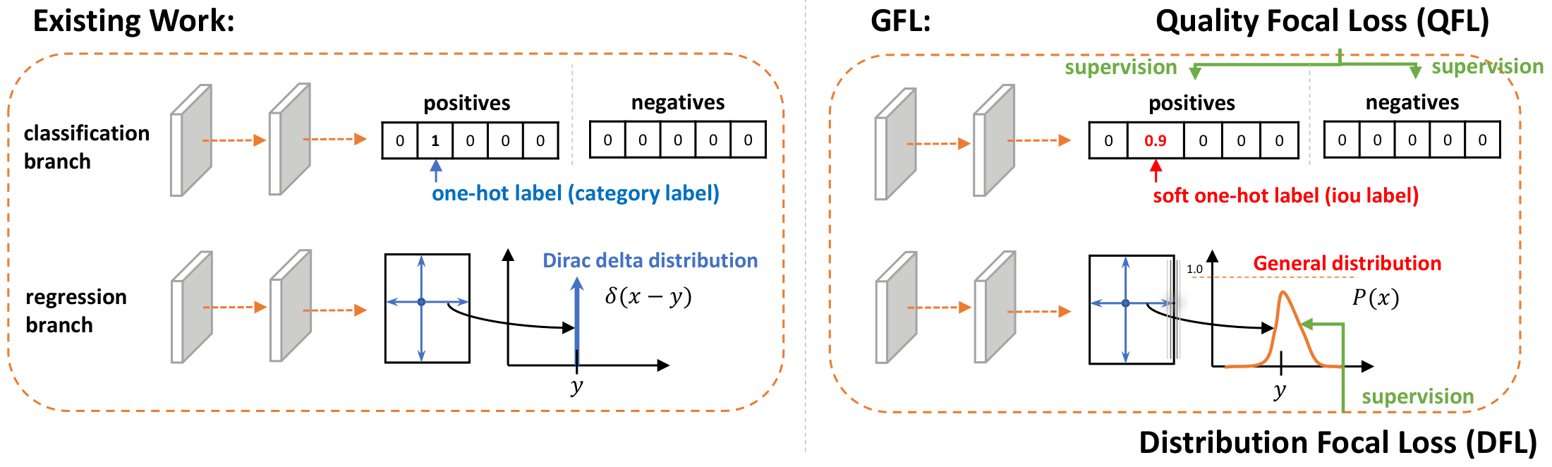
Distribution Focal Loss (DFL). Following [4, 5], we adopt the relative offsets from the location to the four sides of a bounding box as the regression targets (see the regression branch in Figure 4). Conventional operations of bounding box regression model the regressed label $y$ as Dirac delta distribution $\delta(x - y)$, where it satisfies $\int_{-\infty}^{+\infty} \delta(x - y)\mathop{}!\mathrm{d} x = 1$ and is usually implemented through fully connected layers. More formally, the integral form to recover $y$ is as follows:

$ y = \int_{-\infty}^{+\infty} \delta(x - y) x \mathop{}!\mathrm{d} x. $

According to the analysis in Section 1, instead of the Dirac delta [11, 12, 13, 4, 5] or Gaussian [15, 1] assumptions, we propose to directly learn the underlying General distribution $P(x)$ without introducing any other priors. Given the range of label $y$ with minimum $y_0$ and maximum $y_n$ ($y_0 \le y \le y_n, n \in \mathbb{N}^+$), we can have the estimated value $\hat{y}$ from the model ($\hat{y}$ also meets $y_0 \le \hat{y} \le y_n$):

$ \hat{y} = \int_{-\infty}^{+\infty} P(x) x \mathop{}!\mathrm{d} x = \int_{y_0}^{y_n} P(x) x \mathop{}!\mathrm{d} x. $

To be consistent with convolutional neural networks, we convert the integral over the continuous domain into a discrete representation, via discretizing the range $[y_0, y_n]$ into a set ${y_0, y_1, ..., y_i, y_{i+1}, ..., y_{n-1}, y_n}$ with even intervals $\varDelta$ (we use $\varDelta = 1$ for simplicity). Consequently, given the discrete distribution property $\sum_{i = 0}^{n} P(y_i) = 1$, the estimated regression value $\hat{y}$ can be presented as:

$ \hat{y} = \sum_{i = 0}^{n} P(y_i) y_i. $

As a result, $P(x)$ can be easily implemented through a softmax $\mathcal{S(\cdot)}$ layer consisting of $n + 1$ units, with $P(y_i)$ being denoted as $\mathcal{S}i$ for simplicity. Note that $\hat{y}$ can be trained in an end-to-end fashion with traditional loss objectives like SmoothL1 [10], IoU Loss [16] or GIoU Loss [19]. However, there are infinite combinations of values for $P(x)$ that can make the final integral result being $y$, as shown in Figure 5(b), which may reduce the learning efficiency. Intuitively compared against (1) and (2), distribution (3) is compact and tends to be more confident and precise on the bounding box estimation, which motivates us to optimize the shape of $P(x)$ via explicitly encouraging the high probabilities of values that are close to the target $y$. Furthermore, it is often the case that the most appropriate underlying location, if exists, would not be far away from the coarse label. Therefore, we introduce the Distribution Focal Loss (DFL) which forces the network to rapidly focus on the values near label $y$, by explicitly enlarging the probabilities of $y_i$ and $y{i+1}$ (nearest two to $y$, $y_i \le y \le y_{i+1}$). As the learning of bounding boxes are only for positive samples without the risk of class imbalance problem, we simply apply the complete cross entropy part in QFL for the definition of DFL:

$ \textbf{DFL}(\mathcal{S}i, \mathcal{S}{i+1})=-\big((y_{i+1} - y)\log(\mathcal{S}i)+(y - y{i})\log(\mathcal{S}_{i+1})\big). $

Intuitively, DFL aims to focus on enlarging the probabilities of the values around target $y$ (i.e., $y_i$ and $y_{i+1}$). The global minimum solution of DFL, i.e, $\mathcal{S}i = \frac{y{i+1} - y}{y_{i+1} - y_i}, \mathcal{S}{i+1} = \frac{y - y_i}{y{i+1} - y_i}$ (see Supplementary Materials), can guarantee the estimated regression target $\hat{y}$ infinitely close to the corresponding label $y$, i.e., $\hat{y} = \sum_{j = 0}^{n} P(y_j) y_j = \mathcal{S}iy_i + \mathcal{S}{i+1}y_{i+1} = \frac{y_{i+1} - y}{y_{i+1} - y_i} y_i + \frac{y - y_i}{y_{i+1} - y_i} y_{i+1} = y$, which also ensures its correctness as a loss function.

Generalized Focal Loss (GFL). Note that QFL and DFL can be unified into a general form, which is called the Generalized Focal Loss (GFL) in the paper. Assume that a model estimates probabilities for two variables $y_l, y_r (y_l < y_r)$ as $p_{y_l}, p_{y_r}$ ($p_{y_l} \ge 0, p_{y_r} \ge 0, p_{y_l} + p_{y_r}=1$), with a final prediction of their linear combination being $\hat{y} = y_l p_{y_l} + y_r p_{y_r} (y_l \le \hat{y} \le y_r)$. The corresponding continuous label $y$ for the prediction $\hat{y}$ also satisfies $y_l \le y \le y_r$. Taking the absolute distance $|y - \hat{y}|^\beta$ ($\beta \ge 0$) as modulating factor, the specific formulation of GFL can be written as:

$ \textbf{GFL}(p_{y_l}, p_{y_r}) = - \big|y - (y_l p_{y_l} + y_r p_{y_r})\big|^{\beta} \big((y_r - y)\log(p_{y_l}) + (y - y_l)\log(p_{y_r})\big). $

Properties of GFL. $\textbf{GFL}(p_{y_l}, p_{y_r})$ reaches its global minimum with $p_{y_l}^* = \frac{y_r - y}{y_r - y_l}, p_{y_r}^* = \frac{y - y_l}{y_r - y_l}$, which also means that the estimation $\hat{y}$ perfectly matches the continuous label $y$, i.e., $\hat{y} = y_l p_{y_l}^* + y_r p_{y_r}^* = y$ (see the proof in Supplementary Materials). Obviously, the original FL [2] and the proposed QFL and DFL are all special cases of GFL (see Supplementary Materials for details). Note that GFL can be applied to any one-stage detectors. The modified detectors differ from the original detectors in two aspects. First, during inference, we directly feed the classification score (joint representation with quality estimation) as NMS scores without the need of multiplying any individual quality prediction if there exists (e.g., centerness as in FCOS [4] and ATSS [5]). Second, the last layer of the regression branch for predicting each location of bounding boxes now has $n+1$ outputs instead of $1$ output, which brings negligible extra computing cost as later shown in Table 3.

Training Dense Detectors with GFL. We define training loss $\mathcal{L}$ with GFL:

$ \mathcal{L} = \frac{1}{N_{pos}}\sum_{z}{\mathcal{L_{Q}}} + \frac{1}{N_{pos}}\sum_{z} \textbf{1}{{c^*{z} > 0}} \big( \lambda_{0}\mathcal{L_{B}} + \lambda_{1}\mathcal{L_{D}} \big), $

where $\mathcal{L_{Q}}$ is QFL and $\mathcal{L_{D}}$ is DFL. Typically, $\mathcal{L_{B}}$ denotes the GIoU Loss as in [4, 5]. $N_{pos}$ stands for the number of positive samples. $\lambda_0$ (typically 2 as default, similarly in [20]) and $\lambda_1$ (practically $\frac{1}{4}$, averaged over four directions) are the balance weights for $\mathcal{L_{Q}}$ and $\mathcal{L_{D}}$, respectively. The summation is calculated over all locations $z$ on the pyramid feature maps [21]. $\textbf{1}{{c^*{z} > 0}}$ is the indicator function, being 1 if $c^*_{z} > 0$ and 0 otherwise. Following the common practices in the official codes [20, 4, 5, 22], we also utilize the quality scores to weight $\mathcal{L_{B}}$ and $\mathcal{L_{D}}$ during training.

::: {caption="Table 1: Study on QFL (ResNet-50 backbone). All experiments are reproduced in mmdetection [20] and validated on COCO minival."}

:::

4. Experiment

Section Summary: The experiments evaluate the proposed Generalized Focal Loss approach on the standard COCO object detection benchmark, training on 115K images with a ResNet-50 backbone under common settings and reporting results on the 20K-image test set. Ablation studies demonstrate that the Quality Focal Loss produces more reliable joint classification and localization scores than separate or implicit alternatives, while the Distribution Focal Loss yields more accurate bounding-box predictions by modeling uncertainty, with the two components providing complementary gains. Together they improve a strong baseline by roughly 1% AP at negligible extra cost, resulting in a better overall speed-accuracy tradeoff than prior detectors.

Our experiments are conducted on COCO benchmark [24], where trainval35k (115K images) is utilized for training and we use minival (5K images) as validation for our ablation study. The main results are reported on test-dev (20K images) which can be obtained from the evaluation server. For fair comparisons, all results are produced under mmdetection [20], where the default hyper-parameters are adopted. Unless otherwise stated, we adopt 1x learning schedule (12 epochs) without multi-scale training for the following studies, based on ResNet-50 [25] backbone. More training/test details can be found in Supplementary Materials.

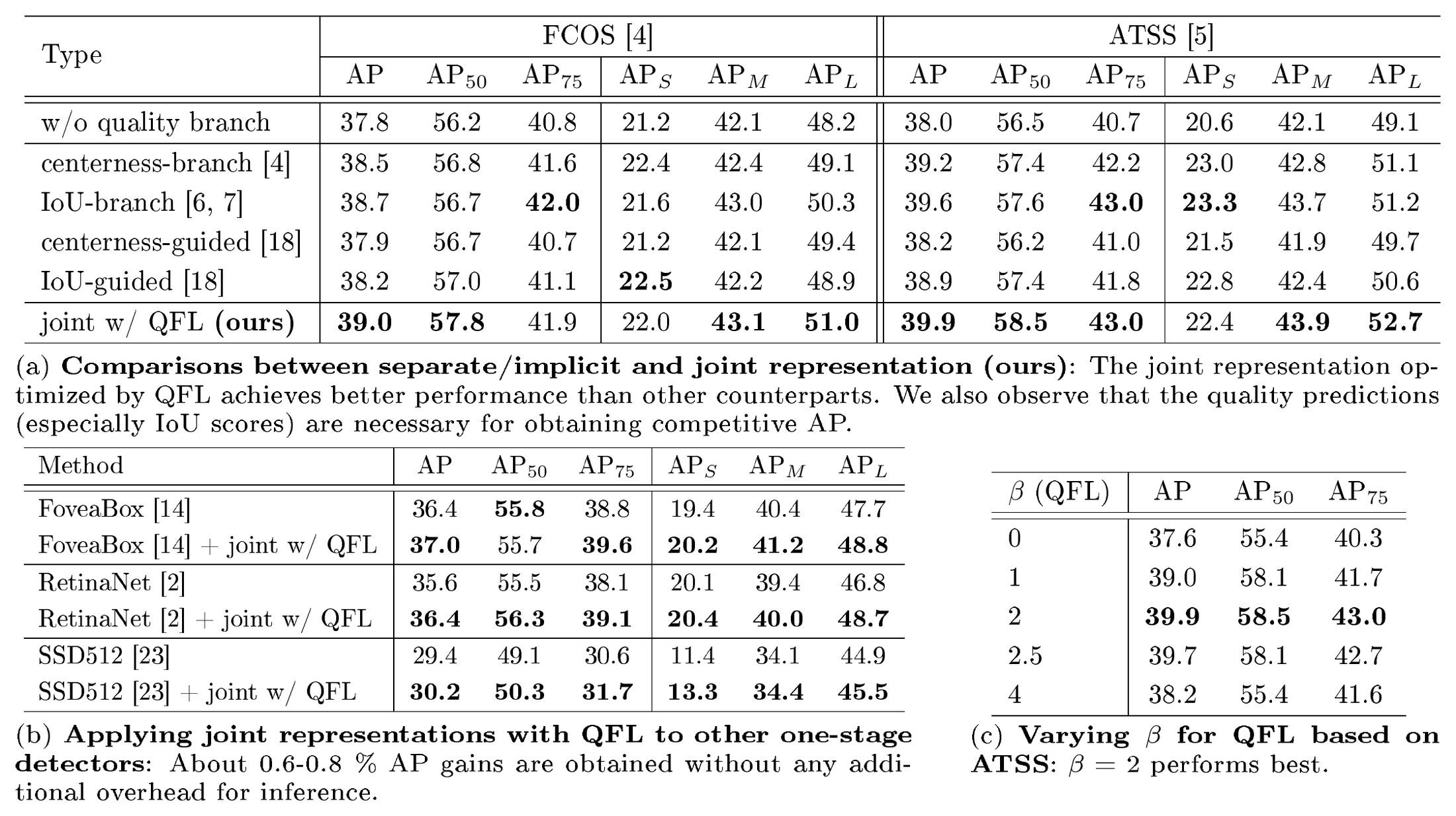
We first investigate the effectiveness of the QFL (Table 1). In Table 1(a), we compare the proposed joint representation with its separate or implicit counterparts. Two alternatives for representing localization quality: IoU [6, 7] and centerness [4, 5] are also adopted in the experiments. In general, we construct 4 variants that use separate or implicit representation, as illustrated in Figure 6. According to the results, we observe that the joint representations optimized by QFL consistently achieve better performance than all the counterparts, whilst IoU always performs better than centerness as a measurement of localization quality (Supplementary Materials). Table 1(b) shows that QFL can also boost the performance of other popular one-stage detectors, and Table 1(c) shows that $\beta = 2$ is the best setting for QFL. We illustrate the effectiveness of joint representation by sampling instances with its predicted classification and IoU scores of both IoU-branch model and ours, as shown in Figure 2(b). It demonstrates that the proposed joint representation trained with QFL can benefit the detection due to its more reliable quality estimation, and yields the strongest correlation between classification and quality scores according to its definition. In fact, in our joint representation, the predicted classification score is equal to the estimated quality score exactly.

::: {caption="Table 2: Study on DFL (ResNet-50 backbone). All experiments are reproduced in mmdetection [20] and validated on COCO minival."}

:::

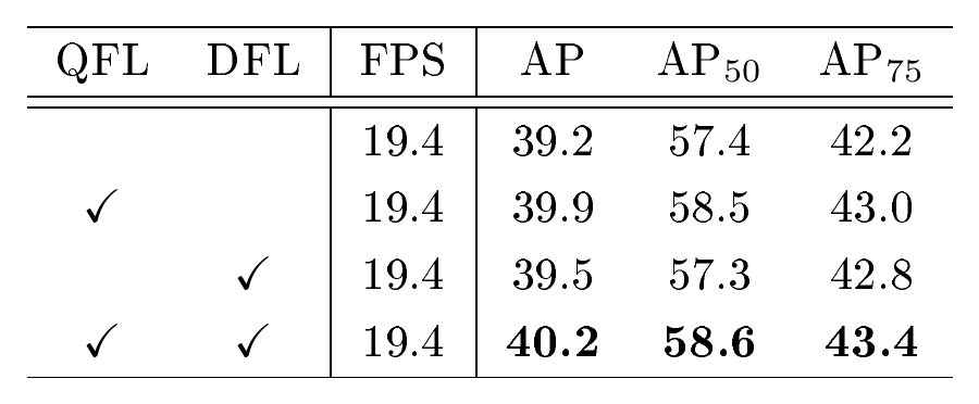
::: {caption="Table 3: The effect of QFL and DFL on ATSS: The effects of QFL and DFL are orthogonal, whilst utilizing both can boost 1% AP over the strong ATSS baseline, without introducing additional overhead practically."}

:::

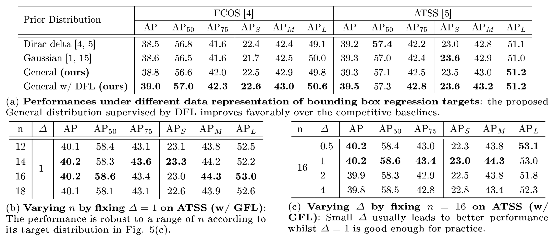
Second, we investigate the effectiveness of the DFL (Table 2). To quickly select a reasonable value of $n$, we first illustrate the distribution of the regression targets in Figure 5(c). We will show in later experiments, the recommended choice of $n$ for ATSS is 14 or 16. In Table 2(a), we compare the effectiveness of different data representations for bounding box regression. We find that the General distribution achieves superior or at least comparable results, whilst DFL can further boost its performance. Qualitative comparisons are depicted in Figure 7. It is observed that the proposed General distribution can provide more accurate bounding box locations than Gaussian and Dirac delta distribution, especially under the case with considerable occlusions (More discussions in Supplementary Materials). Based on the improved ATSS trained by GFL, we report the effect of $n$ and $\varDelta$ in DFL by fixing one and varying another in Table 2(b) and (c). The results demonstrate that the selection of $n$ is not sensitive and $\varDelta$ is suggested to be small (e.g., 1) in practice. To illustrate the effect of General distribution, we plot several representative instances with its distributed bounding box over four directions in Figure 3, where the proposed distributed representation can effectively reflect the uncertainty of bounding boxes by its shape (see more examples in Supplementary Materials).

::: {caption="Table 4: Comparisons between state-of-the-art detectors (single-model and single-scale results) on COCO test-dev. 'MS$_{\text{train}}

:::

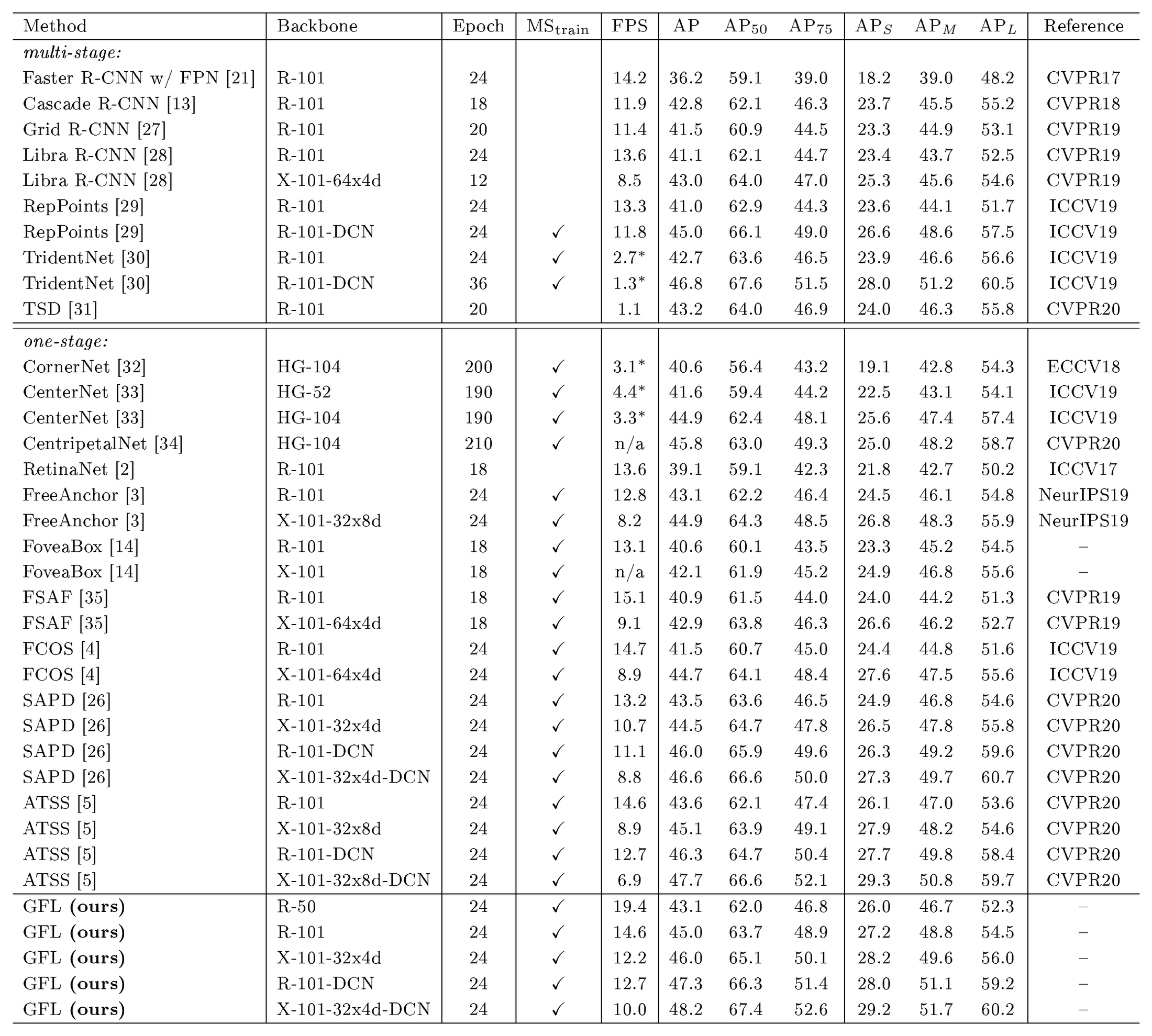
Third, we perform the ablation study on ATSS with ResNet-50 backbone to show the relative contributions of QFL and DFL (Table 3). FPS (Frames-per-Second) is measured on the same machine with a single GeForce RTX 2080Ti GPU using a batch size of 1 under the same mmdetection [20] framework. We observe that the improvement of DFL is orthogonal to QFL, and joint usage of both (i.e., GFL) improves the strong ATSS baseline by absolute 1% AP score. Furthermore, according to the inference speeds, GFL brings negligible additional overhead and is considered very practical.

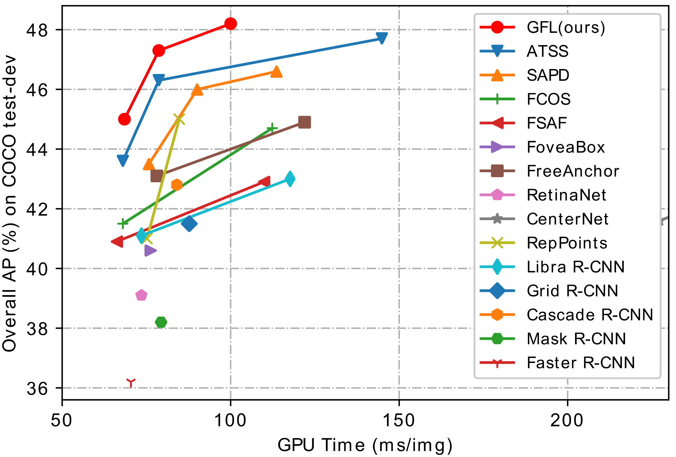
Finally, we compare GFL (based on ATSS) with state-of-the-art approaches on COCO test-dev in Table 4. Following previous works [2, 4], the multi-scale training strategy and 2x learning schedule (24 epochs) are adopted during training. For a fair comparison, we report the results of single-model single-scale testing for all methods, as well as their corresponding inference speeds (FPS). GFL with ResNet-101 [25] achieves 45.0% AP at 14.6 FPS, which is superior than all the existing detectors with the same backbone, including SAPD [26] (43.5%) and ATSS [5] (43.6%). Further, Deformable Convolutional Networks (DCN) [36] consistently boost the performances over ResNe(X)t backbones, where GFL with ResNeXt-101-32x4d-DCN obtains state-of-the-art 48.2% AP at 10 FPS. Figure 8 demonstrates the visualization of the accuracy-speed trade-off, where it can be observed that our proposed GFL pushes the envelope of accuracy-speed boundary to a high level.

5. Conclusion

Section Summary: Researchers have introduced a Generalized Focal Loss method to help object detectors more accurately identify and place boxes around items in images by extending an earlier technique from simple yes-no decisions to a smoother, continuous approach. This method includes two variants, one that better combines object classification with positioning quality and another that models box locations as flexible distributions for greater precision. Experiments confirm the approach works well and could serve as a useful foundation for future detection systems.

To effectively learn qualified and distributed bounding boxes for dense object detectors, we propose Generalized Focal Loss (GFL) that generalizes the original Focal Loss from ${1, 0}$ discrete formulation to the continuous version. GFL can be specialized into Quality Focal loss (QFL) and Distribution Focal Loss (DFL), where QFL encourages to learn a better joint representation of classification and localization quality, and DFL provides more informative and precise bounding box estimations by modeling their locations as General distributions. Extensive experiments validate the effectiveness of GFL. We hope GFL can serve as a simple yet effective baseline for the community.

Appendix

Section Summary: The appendix explores bounding box regression by comparing rigid distributions like Dirac delta and Gaussian to a more flexible General distribution, highlighting how the latter decouples representation from optimization to support both edge-level and IoU-based losses while proving more robust to feature noise. It then mathematically demonstrates that the Generalized Focal Loss reaches a global minimum only at probabilities matching the true IoU between predicted and ground-truth boxes, unlike standard losses whose optima remain one-hot labels. Finally, it shows that Focal Loss and related variants emerge as special cases of this broader formulation.

A. More Discussions about the Distributions

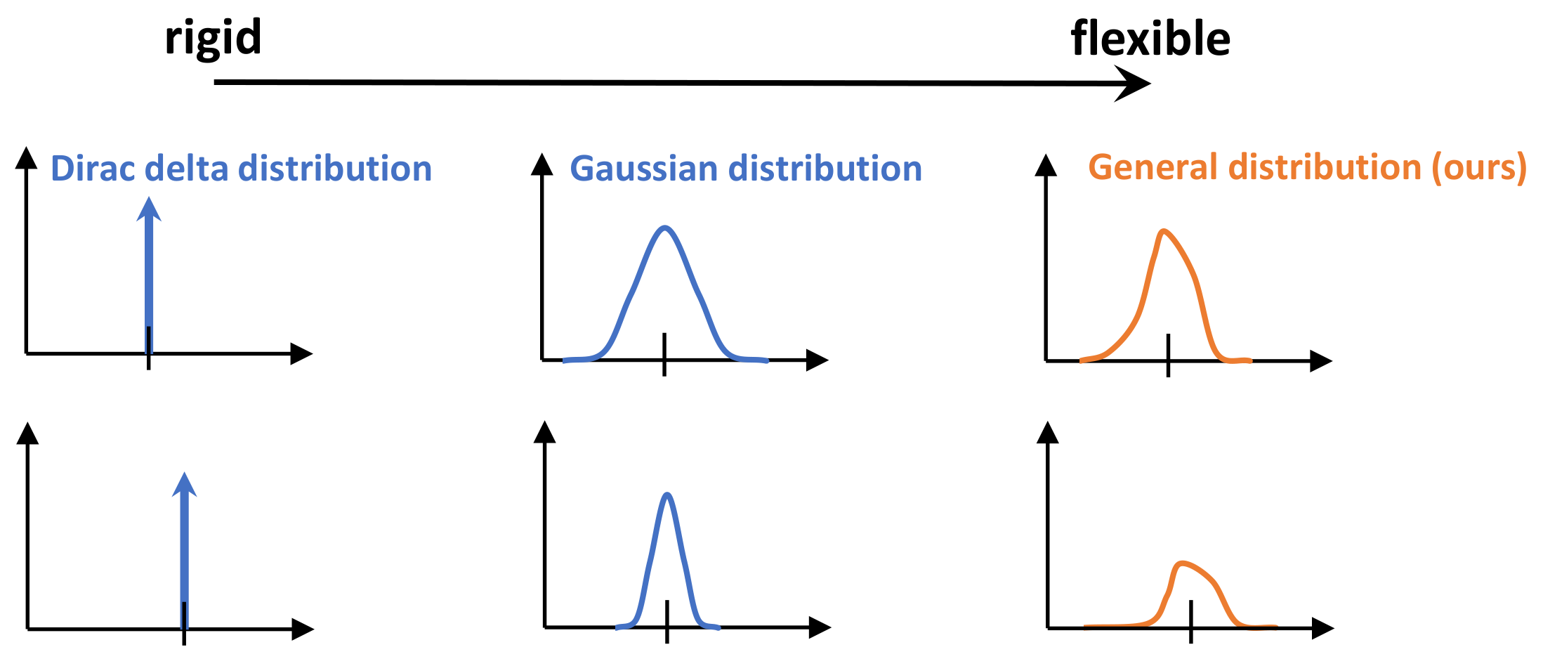
Figure 9 depicts the ideas of Dirac delta, Gaussian, and the proposed General distributions, where the assumption goes from rigid (Dirac delta) to flexible (General). We also list several key comparisons about these distributions in Table 5. It can be observed that the loss objective of the Gaussian assumption is actually a dynamically weighted L2 Loss, where its training weight is related to the predicted variance $\sigma$. It is somehow similar to that of Dirac delta (standard L2 Loss) when optimized at the edge level. Moreover, it is not clear how to integrate the Gaussian assumption into the IoU-based Loss formulations, since it heavily couples the expression of the target representation with its optimization objective. Therefore, it can not enjoy the benefits of the IoU-based optimization [19], as it is proved to be very effective in practice. In contrast, our proposed General distribution decouples the representation and loss objective, making it feasible for any type of optimizations, including both edge level and box level.

::: {caption="Table 5: Comparisons between three distributions. 'edge' level denotes optimization over four respective directions, whilst 'box' level means IoU-based Losses [19] that consider the bounding box as a whole."}

:::

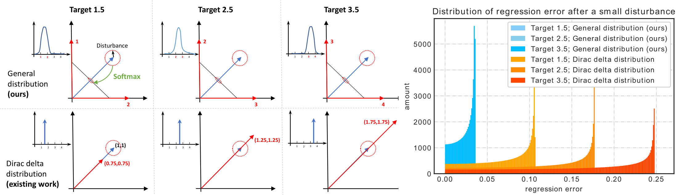
We also find that the bounding box regression of Dirac delta distribution (including Gaussian distribution based on the analysis from Table 5) behaves more sensitive to feature perturbations, making it less robust and susceptible to noise, as shown in the simulation experiment (Figure 10). It proves that General distribution enjoys more benefits than the other counterparts.

B. Global Minimum of $\textbf{GFL}(p_{y_l}, p_{y_r})$

Let's review the definition of $\textbf{GFL}$:

$ \textbf{GFL}(p_{y_l}, p_{y_r}) = - \big|y - (y_l p_{y_l} + y_r p_{y_r})\big|^{\beta} \big((y_r - y)\log(p_{y_l}) + (y - y_l)\log(p_{y_r})\big), \ \ \ \text{given}\ \ p_{y_l} + p_{y_r} = 1. \nonumber $

For simplicity, $\textbf{GFL}(p_{y_l}, p_{y_r})$ can then be expanded as:

$ \begin{aligned}\textbf{GFL}(p_{y_l}, p_{y_r}) & = - \big|y - (y_l p_{y_l} + y_r p_{y_r})\big|^{\beta} \big((y_r - y)\log(p_{y_l}) + (y - y_l)\log(p_{y_r})\big)\& = \underbrace{\left{ \big|y - (y_l p_{y_l} + y_r p_{y_r})\big|^{\beta}\right}}{\textbf{L}(\cdot,\cdot)} \underbrace{\left{ -\big((y_r - y)\log(p{y_l}) + (y - y_l)\log(p_{y_r})\big)\right}}{\textbf{R}(\cdot,\cdot)}\& = \textbf{L}(p{y_l}, p_{y_r}) \textbf{R}(p_{y_l}, p_{y_r}), \nonumber\end{aligned} $

$ \begin{aligned}\textbf{R}(p_{y_l}, p_{y_r}) &= -\big((y_r - y)\log(p_{y_l}) + (y - y_l)\log(p_{y_r})\big)\& = -\big((y_r - y)\log(p_{y_l}) + (y - y_l)\log(1 - p_{y_l})\big)\& \ge -\big( (y_r - y)\log(\frac{y_r - y}{y_r - y_l}) + (y - y_l)\log(\frac{y - y_l}{y_r - y_l}) \big)\& = \textbf{R}(p_{y_l}^*, p_{y_r}^*) > 0, \ \ \ \text{where}\ \ \ p_{y_l}^* = \frac{y_r - y}{y_r - y_l}, p_{y_r}^* = \frac{y - y_l}{y_r - y_l}.\\textbf{L}(p_{y_l}, p_{y_r}) &= \big|y - (y_l p_{y_l} + y_r p_{y_r})\big|^{\beta}\& \ge \textbf{L}(p_{y_l}^*, p_{y_r}^*) = 0, \ \ \ \text{where}\ \ \ p_{y_l}^* = \frac{y_r - y}{y_r - y_l}, p_{y_r}^* = \frac{y - y_l}{y_r - y_l}. \nonumber\end{aligned} $

Furthermore, given $\epsilon \neq 0$, for arbitrary variable $(p_{y_l}, p_{y_r}) = (p_{y_l}^* + \epsilon, p_{y_r}^* - \epsilon)$ in the domain of definition, we can have:

$ \begin{aligned} \textbf{R}(p_{y_l}^* + \epsilon, p_{y_r}^* - \epsilon) > \textbf{R}(p_{y_l}, p_{y_r}) > 0, \ \textbf{L}(p_{y_l}^* + \epsilon, p_{y_r}^* - \epsilon) = \big|\epsilon(y_r - y_l)\big|^{\beta} > 0 = \textbf{L}(p_{y_l}^*, p_{y_r}^*). \nonumber \end{aligned} $

Therefore, it is easy to deduce:

$ \begin{aligned} \textbf{GFL}(p_{y_l}, p_{y_r}) & = \textbf{L}(p_{y_l}, p_{y_r}) \textbf{R}(p_{y_l}, p_{y_r}) \ge \textbf{L}(p_{y_l}^*, p_{y_r}^*)\textbf{R}(p_{y_l}^*, p_{y_r}^*) = 0, \nonumber \end{aligned} $

where "$=

The global minimum property of GFL somehow explains why the IoU or centerness guided variants in Figure 6 would not have obvious advantages. In fact, the weighted guidance does not essentially change the global minimum of the original classification loss (e.g., Focal Loss), whilst their optimal classification targets are still one-hot labels. In contrast, the proposed GFL indeed modifies the global minimum and force the predictions to approach the accurate IoU between the estimated boxes and ground-truth boxes, which is obviously beneficial for the rank process of NMS.

C. FL, QFL and DFL are special cases of GFL

In this section, we show how GFL can be specialized into the form of FL, QFL and DFL, respectively.

FL: Letting $\beta = \gamma, y_l = 0, y_r = 1, p_{y_r} = p, p_{y_l} = 1 - p$ and $y \in {1, 0}$ in GFL, we can obtain FL:

$ \begin{aligned} \textbf{FL}(p) &= \textbf{GFL}(1-p, p)= -\big|y - p\big|^{\gamma} \big((1 - y)\log(1 - p) + y\log(p)\big), y \in {1, 0} \ & = -(1 - p_t)^\gamma\log(p_t), p_t = \left{\begin{array}{rc}p, & \text{when}\ \ y = 1 \1 - p, & \text{when}\ \ y = 0\end{array} \right. \end{aligned} $

QFL: Having $y_l = 0, y_r = 1, p_{y_r} = \sigma$ and $p_{y_l} = 1 - \sigma$ in GFL, the form of QFL can be written as:

$ \textbf{QFL}(\sigma) = \textbf{GFL}(1-\sigma, \sigma) = -\big|y - \sigma\big|^{\beta}\big((1 - y)\log(1 - \sigma) + y\log(\sigma)\big). $

DFL: By substituting $\beta = 0, y_l = y_i, y_r = y_{i+1}, p_{y_l} = P(y_l) = P(y_i) = \mathcal{S}i, p{y_r} = P(y_r) = P(y_{i+1}) = \mathcal{S}_{i+1}$ in GFL, we can have DFL:

$ \textbf{DFL}(\mathcal{S}i, \mathcal{S}{i+1})=\textbf{GFL}(\mathcal{S}i, \mathcal{S}{i+1})=-\big((y_{i+1} - y)\log(\mathcal{S}i)+(y - y{i})\log(\mathcal{S}_{i+1})\big). $

D. Details of Experimental Settings

Training Details: The ImageNet pretrained models [25] with FPN [21] are utilized as the backbones. During training, the input images are resized to keep their shorter side being 800 and their longer side less or equal to 1333. In ablation study, the networks are trained using the Stochastic Gradient Descent (SGD) algorithm for 90K iterations (denoted as 1x schedule) with 0.9 momentum, 0.0001 weight decay and 16 batch size. The initial learning rate is set as 0.01 and decayed by 0.1 at iteration 60K and 80K, respectively.

Inference Details: During inference, the input image is resized in the same way as in the training phase, and then passed through the whole network to output the predicted bounding boxes with a predicted class. Then we use the threshold 0.05 to filter out a variety of backgrounds, and output top 1000 candidate detections per feature pyramid. Finally, NMS is applied under the IoU threshold 0.6 per class to produce the final top 100 detections per image as results.

E. Why is IoU-branch always superior than centerness-branch?

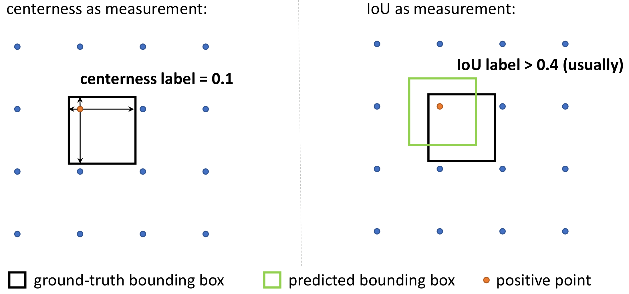
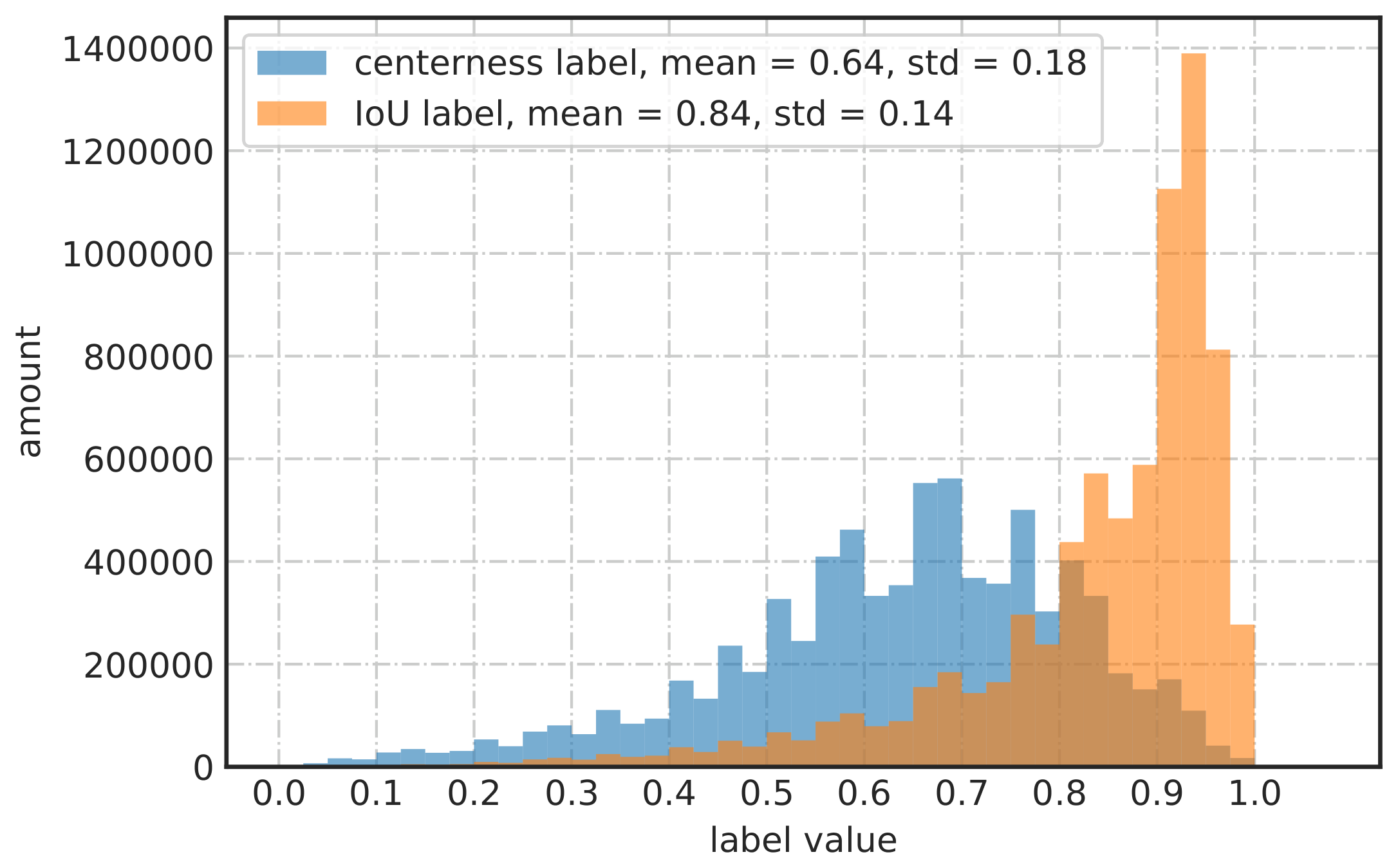
The ablation study in original paper also demonstrates that for FCOS/ATSS, IoU performs consistently better than centerness, as a measurement of localization quality. Here we give a convincing reason why this is the case. We discover the major problem of centerness is that its definition leads to unexpected small ground-truth label, which makes a possible set of ground-truth bounding boxes extremely hard to be recalled (as shown in Figure 11). From the label distributions demonstrated in Figure 12, we observe that most of IoU labels is larger than 0.4 yet centerness labels tend to be much smaller (even approaching 0). The small values of centerness labels prevent a set of ground-truth bounding boxes from being recalled, as their final scores for NMS would be potentially small since their predicted centerness scores are already supervised by these extremely small signals.

F. More Examples of Distributed Bounding Boxes

We demonstrate more examples with General distributed bounding boxes predicted by GFL (ResNet-50 backbone). As demonstrated in Figure 13, we show several cases with boundary ambiguities: does the slim and almost invisible backpack strap belong to the box of the bag (left top)? does the partially occluded umbrella handle belong to the entire umbrella (left down)? In these cases, our models even produce more reasonable coordinates of bounding boxes than the ground-truth ones. In Figure 14, more examples with clear boundaries and sharp General distributions are shown, where GFL is very confident to generate accurate bounding boxes, e.g., the bottom parts of the orange and skiing woman.

:::: {.figure cols="1"}

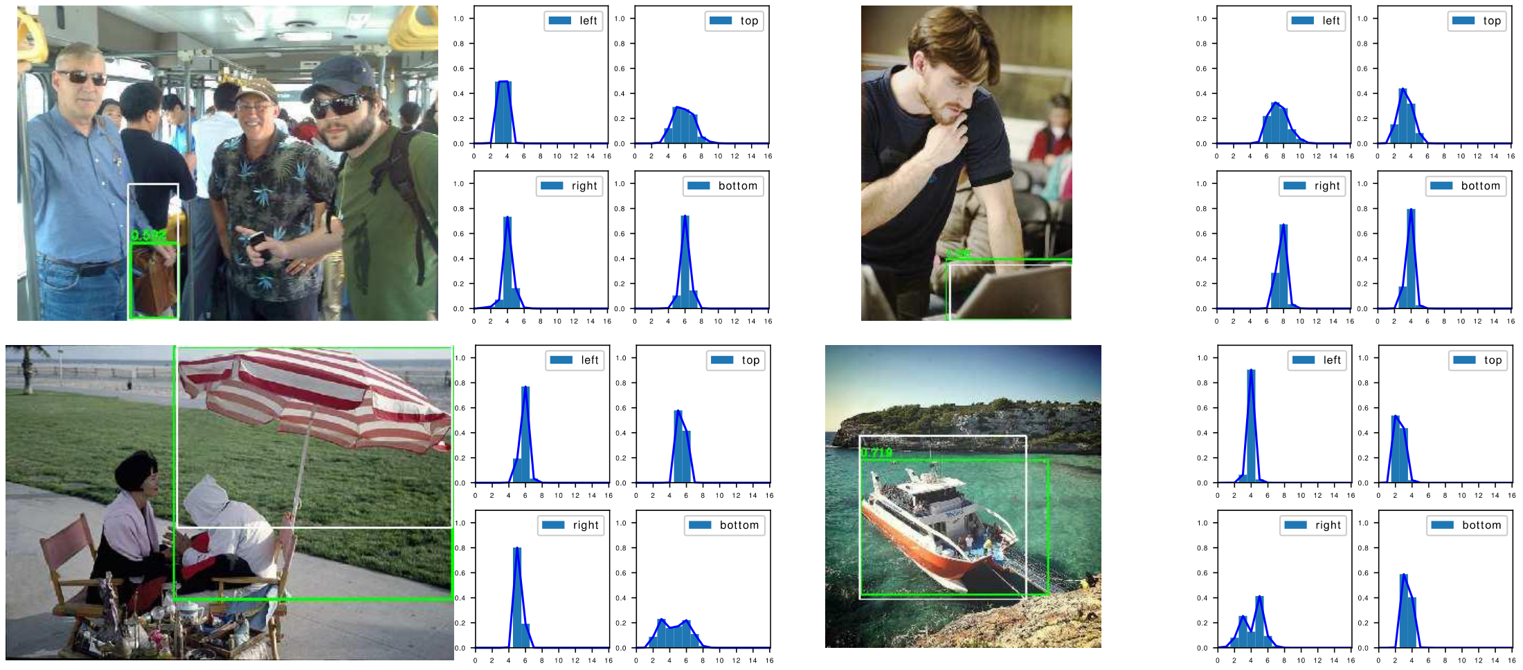
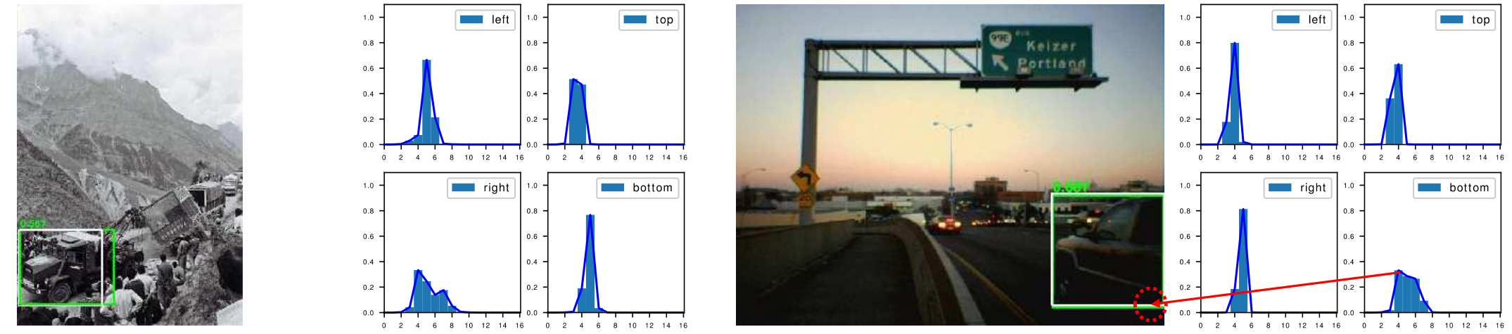
Figure 13: Examples with huge boundary ambiguities and uncertainties, where the learned General distributions tend to be flatten. In some cases, we even observe a distribution with two peaks. Interestingly, they do correspond to two different most likely boundaries in the image, e.g., the boundaries of the umbrella whether its heavily occluded handle is considered. Predictions are marked green in images, whilst ground-truth boxes are white. ::::

:::: {.figure cols="1"}

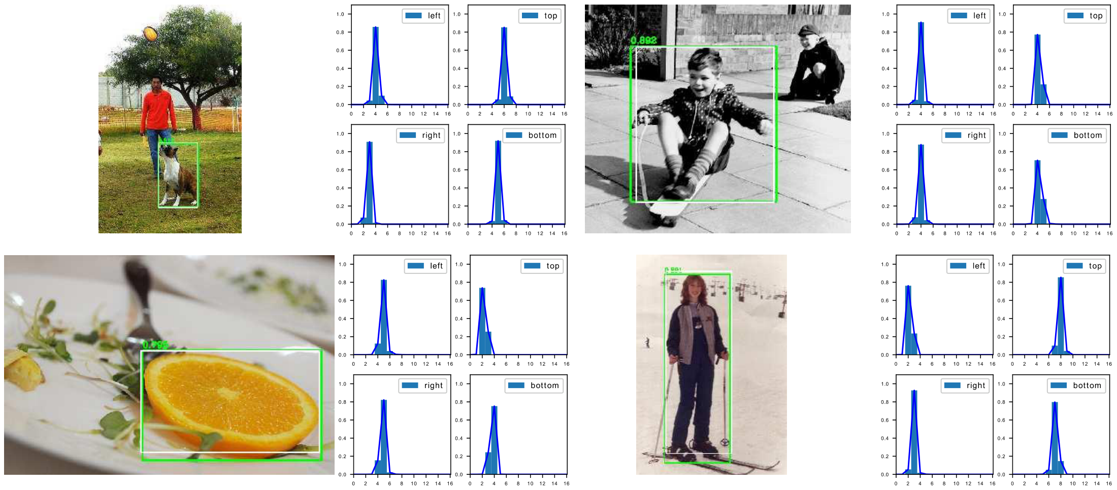
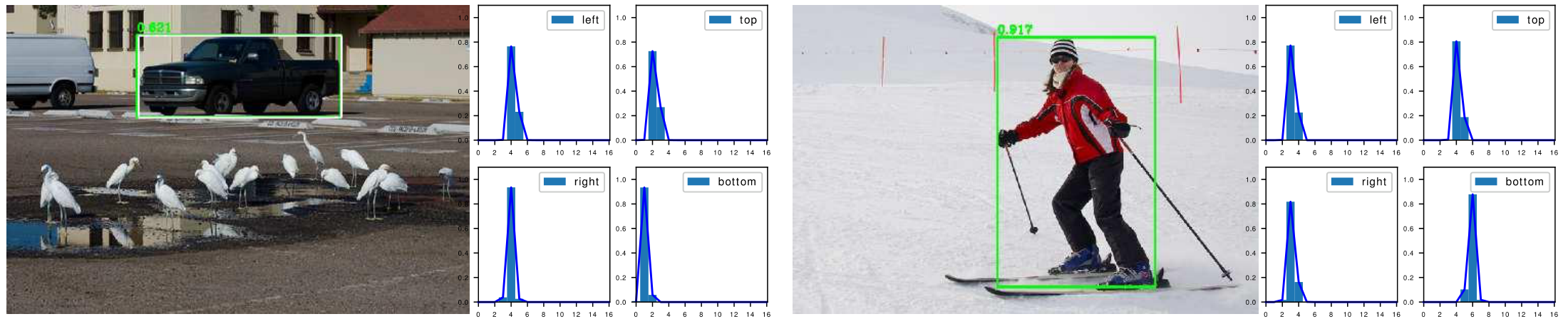
Figure 14: Examples with extremely clear boundaries. The learned General distributions are relatively sharp whilst producing very accurate box estimations. Predictions are marked green in images, whilst ground-truth boxes are white. ::::

References

Section Summary: This section compiles a bibliography of research papers primarily on object detection methods in computer vision, spanning techniques for improving bounding box accuracy, handling anchors, and refining single-stage or two-stage detectors. The citations draw from major conferences such as CVPR, ICCV, and NeurIPS, along with some arXiv preprints, and reference foundational works on datasets like COCO and tools like MMDetection. Overall, they represent key contributions from recent years aimed at making object recognition more precise and efficient.

[1] Yihui He, Chenchen Zhu, Jianren Wang, Marios Savvides, and Xiangyu Zhang. Bounding box regression with uncertainty for accurate object detection. In CVPR, 2019.

[2] Tsung-Yi Lin, Priya Goyal, Ross Girshick, Kaiming He, and Piotr Dollár. Focal loss for dense object detection. In ICCV, 2017.

[3] Xiaosong Zhang, Fang Wan, Chang Liu, Rongrong Ji, and Qixiang Ye. Freeanchor: Learning to match anchors for visual object detection. In NeurIPs, 2019.

[4] Zhi Tian, Chunhua Shen, Hao Chen, and Tong He. Fcos: Fully convolutional one-stage object detection. In ICCV, 2019.

[5] Shifeng Zhang, Cheng Chi, Yongqiang Yao, Zhen Lei, and Stan Z Li. Bridging the gap between anchor-based and anchor-free detection via adaptive training sample selection. In CVPR, 2020.

[6] Shengkai Wu, Xiaoping Li, and Xinggang Wang. Iou-aware single-stage object detector for accurate localization. Image and Vision Computing, 2020.

[7] Borui Jiang, Ruixuan Luo, Jiayuan Mao, Tete Xiao, and Yuning Jiang. Acquisition of localization confidence for accurate object detection. In ECCV, 2018.

[8] Zhaojin Huang, Lichao Huang, Yongchao Gong, Chang Huang, and Xinggang Wang. Mask scoring r-cnn. In CVPR, 2019.

[9] Li Zhu, Zihao Xie, Liman Liu, Bo Tao, and Wenbing Tao. Iou-uniform r-cnn: Breaking through the limitations of rpn. arXiv preprint arXiv:1912.05190, 2019.

[10] Ross Girshick. Fast r-cnn. In ICCV, 2015.

[11] Shaoqing Ren, Kaiming He, Ross Girshick, and Jian Sun. Faster r-cnn: Towards real-time object detection with region proposal networks. In NeurIPs, 2015.

[12] Kaiming He, Georgia Gkioxari, Piotr Dollár, and Ross Girshick. Mask r-cnn. In ICCV, 2017.

[13] Zhaowei Cai and Nuno Vasconcelos. Cascade r-cnn: Delving into high quality object detection. In CVPR, 2018.

[14] Tao Kong, Fuchun Sun, Huaping Liu, Yuning Jiang, and Jianbo Shi. Foveabox: Beyond anchor-based object detector. arXiv preprint arXiv:1904.03797, 2019.

[15] Jiwoong Choi, Dayoung Chun, Hyun Kim, and Hyuk-Jae Lee. Gaussian yolov3: An accurate and fast object detector using localization uncertainty for autonomous driving. In ICCV, 2019.

[16] Lachlan Tychsen-Smith and Lars Petersson. Improving object localization with fitness nms and bounded iou loss. In CVPR, 2018.

[17] Yuhang Cao, Kai Chen, Chen Change Loy, and Dahua Lin. Prime sample attention in object detection. arXiv preprint arXiv:1904.04821, 2019.

[18] Shengkai Wu and Xiaoping Li. Iou-balanced loss functions for single-stage object detection. arXiv preprint arXiv:1908.05641, 2019.

[19] Hamid Rezatofighi, Nathan Tsoi, JunYoung Gwak, Amir Sadeghian, Ian Reid, and Silvio Savarese. Generalized intersection over union: A metric and a loss for bounding box regression. In CVPR, 2019.

[20] Kai Chen, Jiaqi Wang, Jiangmiao Pang, Yuhang Cao, Yu Xiong, Xiaoxiao Li, Shuyang Sun, Wansen Feng, Ziwei Liu, Jiarui Xu, et al. Mmdetection: Open mmlab detection toolbox and benchmark. arXiv preprint arXiv:1906.07155, 2019.

[21] Tsung-Yi Lin, Piotr Dollár, Ross Girshick, Kaiming He, Bharath Hariharan, and Serge Belongie. Feature pyramid networks for object detection. In CVPR, 2017.

[22] Hengduo Li, Zuxuan Wu, Chen Zhu, Caiming Xiong, Richard Socher, and Larry S Davis. Learning from noisy anchors for one-stage object detection. arXiv preprint arXiv:1912.05086, 2019.

[23] Wei Liu, Dragomir Anguelov, Dumitru Erhan, Christian Szegedy, Scott Reed, Cheng-Yang Fu, and Alexander C Berg. Ssd: Single shot multibox detector. In ECCV, 2016.

[24] Tsung-Yi Lin, Michael Maire, Serge Belongie, James Hays, Pietro Perona, Deva Ramanan, Piotr Dollár, and C Lawrence Zitnick. Microsoft coco: Common objects in context. In ECCV, 2014.

[25] Kaiming He, Xiangyu Zhang, Shaoqing Ren, and Jian Sun. Deep residual learning for image recognition. In CVPR, 2016.

[26] Chenchen Zhu, Fangyi Chen, Zhiqiang Shen, and Marios Savvides. Soft anchor-point object detection. In CVPR, 2020.

[27] Xin Lu, Buyu Li, Yuxin Yue, Quanquan Li, and Junjie Yan. Grid r-cnn. In CVPR, 2019.

[28] Jiangmiao Pang, Kai Chen, Jianping Shi, Huajun Feng, Wanli Ouyang, and Dahua Lin. Libra r-cnn: Towards balanced learning for object detection. In CVPR, 2019.

[29] Ze Yang, Shaohui Liu, Han Hu, Liwei Wang, and Stephen Lin. Reppoints: Point set representation for object detection. In ICCV, 2019.

[30] Yanghao Li, Yuntao Chen, Naiyan Wang, and Zhaoxiang Zhang. Scale-aware trident networks for object detection. In ICCV, 2019.

[31] Guanglu Song, Yu Liu, and Xiaogang Wang. Revisiting the sibling head in object detector. In CVPR, 2020.

[32] Hei Law and Jia Deng. Cornernet: Detecting objects as paired keypoints. In ECCV, 2018.

[33] Kaiwen Duan, Song Bai, Lingxi Xie, Honggang Qi, Qingming Huang, and Qi Tian. Centernet: Keypoint triplets for object detection. In ICCV, 2019.

[34] Zhiwei Dong, Guoxuan Li, Yue Liao, Fei Wang, Pengju Ren, and Chen Qian. Centripetalnet: Pursuing high-quality keypoint pairs for object detection. In CVPR, 2020.

[35] Chenchen Zhu, Yihui He, and Marios Savvides. Feature selective anchor-free module for single-shot object detection. In CVPR, 2019.

[36] Xizhou Zhu, Han Hu, Stephen Lin, and Jifeng Dai. Deformable convnets v2: More deformable, better results. In CVPR, 2019.