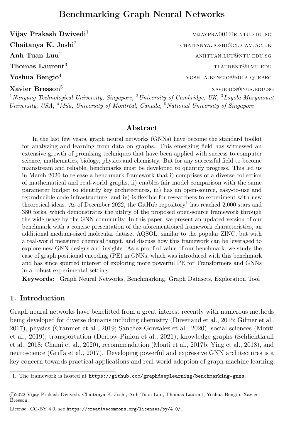
Benchmarking Graph Neural Networks

Vijay Prakash DwivediChaitanya K. JoshiAnh Tuan LuuThomas LaurentYoshua BengioXavier Bresson

article2023JMLR1,147 citationsBest Paper Award

Establishes a standardized benchmarking suite with diverse datasets and strictly controlled parameter budgets to enable fair, reproducible evaluations across graph neural network architectures and positional encoding strategies.

Listen

Graph neural networks have become a vital tool for machine learning across chemistry, physics, social networks, and optimization. However, tracking progress has been historically difficult due to reliance on small legacy datasets, inconsistent evaluation settings, and arbitrary model parameter sizes. These shortcomings made it hard to determine whether performance gains came from true architectural advances or extra parameter capacity. To establish rigorous standards, the article introduces a reproducible, open-source benchmarking framework designed to evaluate graph architectures fairly under fixed parameter budgets across diverse, medium-scale tasks.

To conduct these evaluations, the article curates twelve medium-scale datasets spanning molecular chemistry, social networks, computer vision, and mathematical modeling, covering node, edge, and whole-graph prediction tasks. The framework enforces strict fairness by constraining model complexity to fixed budgets of approximately 100,000 and 500,000 parameters. It compares standard message-passing models, such as vanilla graph convolutional networks and attention-based networks, against theoretically expressive higher-order Weisfeiler-Lehman networks across identical training and hardware configurations.

The experimental findings show that message-passing architectures consistently outperform higher-order networks on medium-scale benchmarks while scaling far more effectively. Anisotropic models that leverage directional attention and edge gating, such as Gated Graph ConvNets and Graph Attention Networks, achieved top performance across multiple domains, outperforming isotropic models on tasks like the Travelling Salesman Problem and collaboration link prediction. In contrast, higher-order networks suffered from high computational and memory complexity, frequently running out of memory or failing to converge when scaled to deeper layers. In addition, the article demonstrated that adding Laplacian positional encodings—derived from graph eigenvectors—dramatically improves message-passing models, raising cycle detection accuracy from baseline levels to over 99% and enabling standard architectures to overcome fundamental symmetry limitations.

These results demonstrate that theoretical expressiveness does not automatically translate to practical success if models cannot scale or train stably using standard deep learning practices like batch normalization. For organizations investing in graph learning, prioritizing computationally efficient message-passing architectures augmented with attention mechanisms and positional encodings offers superior accuracy, lower computational cost, and faster turnaround times. Standardizing parameter budgets also provides an objective method to assess true algorithmic quality rather than superficial gains from model size.

Practitioners and researchers should adopt standardized parameter budgets and integrate Laplacian positional encodings or attention-based mechanisms into their graph pipelines. Before deploying higher-order architectures in production, teams must address their memory and training stability limitations. Future work should focus on principled graph normalization methods, specialized hardware handling for large dense graphs, and refining positional encoding techniques to handle arbitrary sign ambiguities.

  • Paper: Pitfalls of Graph Neural Network Evaluation, Oleksandr Shchur et al. (2018). This foundational critique highlights the widespread flaws and ranking instability of early GNN evaluation practices, directly establishing the methodological need for standardized benchmarks.
  • Paper: Open Graph Benchmark: Datasets for Machine Learning on Graphs, Weihua Hu et al. (2020). This seminal benchmark suite provides critical context for modern large-scale, split-driven graph neural network evaluation standards that parallel and contextualize the benchmark design.
  • Paper: How Powerful are Graph Neural Networks?, Keyulu Xu et al. (2019). It formalizes the Weisfeiler-Lehman theoretical limits and expressive capabilities of standard message-passing architectures evaluated systematically within the benchmark.
  • Paper: Neural Message Passing for Quantum Chemistry, Justin Gilmer et al. (2017). It unifies spatial graph architectures into the Message Passing Neural Network framework, which serves as the core paradigm tested across the benchmark's mathematical and chemical datasets.
  • Paper: Semi-Supervised Classification with Graph Convolutional Networks, Thomas N. Kipf et al. (2017). It introduces Graph Convolutional Networks, serving as a primary baseline architecture evaluated under controlled parameter budgets.
  • Paper: Graph Attention Networks, Petar Veličković et al. (2018). It defines Graph Attention Networks, another essential baseline architecture rigorously compared across the benchmark tasks.
  • Paper: Inductive Representation Learning on Large Graphs, William L. Hamilton et al. (2017). It introduces GraphSAGE and inductive neighborhood aggregation, establishing an important reference model assessed in the comparative experiments.
  • Paper: Fast Graph Representation Learning with PyTorch Geometric, Matthias Fey et al. (2019). It details PyTorch Geometric, the primary open-source deep learning framework on top of which standardized GNN benchmarking suites are implemented.
  • Paper: MoleculeNet: a benchmark for molecular machine learning, Zhenqin Wu et al. (2017). It establishes standardized molecular machine learning evaluation protocols that motivated the inclusion and format of chemical datasets like ZINC and AQSOL.
  • Paper: Do Transformers Really Perform Badly for Graph Representation?, Chengxuan Ying et al. (2021). It demonstrates how graph structural encodings empower Transformer architectures on graph tasks, building upon the positional encoding paradigms explored in the benchmark.
Cover for Benchmarking Graph Neural Networks

Abstract

In the last few years, graph neural networks (GNNs) have become the standard toolkit for analyzing and learning from data on graphs. This emerging field has witnessed an extensive growth of promising techniques that have been applied with success to computer science, mathematics, biology, physics and chemistry. But for any successful field to become mainstream and reliable, benchmarks must be developed to quantify progress. This led us in March 2020 to release a benchmark framework that i) comprises of a diverse collection of mathematical and real-world graphs, ii) enables fair model comparison with the same parameter budget to identify key architectures, iii) has an open-source, easy-to-use and reproducible code infrastructure, and iv) is flexible for researchers to experiment with new theoretical ideas. As of December 2022, the GitHub repository has reached 2,000 stars and 380 forks, which demonstrates the utility of the proposed open-source framework through the wide usage by the GNN community. In this paper, we present an updated version of our benchmark with a concise presentation of the aforementioned framework characteristics, an additional medium-sized molecular dataset AQSOL, similar to the popular ZINC, but with a real-world measured chemical target, and discuss how this framework can be leveraged to explore new GNN designs and insights. As a proof of value of our benchmark, we study the case of graph positional encoding (PE) in GNNs, which was introduced with this benchmark and has since spurred interest of exploring more powerful PE for Transformers and GNNs in a robust experimental setting.

Table of Contents

  • 1 Introduction
  • 2 Overview of GNN Benchmarking Framework
  • 3 How can the benchmark be used to explore new insights?
  • 4 Conclusion
  • A Related Work
  • B Graph Neural Network Pipeline
  • B.1 Message-Passing GCNs
  • B.1.1 Input Layer
  • B.1.2 GCN layers
  • B.1.3 Task-based Layer
  • B.2 Weisfeiler-Lehman GNNs
  • B.2.1 Input Tensor
  • B.2.2 WL-GNN layers
  • B.2.3 Task-based network layers
  • C Datasets and Benchmarking Experiments
  • C.1 Graph Regression with ZINC dataset
  • C.2 Graph Regression with AQSOL dataset
  • C.3 Link Prediction with OGBL-COLLAB dataset
  • C.4 Node Classification with WikiCS dataset
  • C.5 Graph Classification with Super-pixel (MNIST/CIFAR10) datasets
  • C.6 Node Classification with SBM (PATTERN/CLUSTER) datasets
  • C.7 Edge Classification/Link Prediction with TSP dataset
  • C.8 Graph Classification and Isomorphism Testing with CSL dataset
  • C.9 Cycle Detection with CYCLES dataset
  • C.10 Multi-task graph properties with GraphTheoryProp dataset
  • D Analysis and Discussion of Benchmarking Results
  • E Studies using the Benchmarking Framework
  • E.1 Laplacian Positional Encodings
  • E.1.1 Related Work
  • E.1.2 Laplacian eigenvectors as Positional Encodings
  • E.1.3 Experiments and Analysis
  • E.1.4 Challenges with using Laplacian eigenvectors
  • E.2 Edge representations for link prediction.
  • E.2.1 With GatedGCN and GAT
  • E.2.2 With GraphSage
  • F Experiments on TU datasets
  • G A Note on Graph Size Normalization
  • H Elaboration on Benchmarking Design Choices
  • I Hardware
  • J Memory Usage
  • References

Knowls

  1. Knowl 1 — GNN Benchmarking Suite and Standardized Evaluation Protocol

    experimental setup

    To evaluate graph neural networks (GNNs) reliably and differentiate model capabilities on academic-scale compute, the benchmark establishes a collection of 12 medium-scale datasets spanning diverse domains, task levels (graph regression, graph classification, node classification, and edge classification/link prediction), and construction types (real-world and synthetic mathematical graphs):

    • ZINC (12,000 graphs, average 23.16 nodes, 49.83 edges): Graph regression to predict constrained molecular solubility log⁡P−SA−cycle\log P - \text{SA} - \text{cycle}. Node features: 28 atom types; Edge features: 4 bond types. Metric: Mean Absolute Error (MAE).
    • AQSOL (9,823 graphs, average 17.57 nodes, 35.76 edges): Graph regression to predict experimental aqueous solubility (in LogS\text{LogS} units) from AqSolDB using an 8:1:1 scaffold split. Node features: 65 atom types; Edge features: 5 bond types. Metric: MAE.
    • OGBL-COLLAB (1 graph, 235,868 nodes, 2,358,104 edges): Link prediction on an academic collaboration network with temporal edges. Node features: 128-dimensional paper word embeddings; Edge features: 2-dimensional collaboration year and weight. Metric: Hits@50.
    • WikiCS (1 graph, 11,701 nodes, 216,123 edges, 10 classes): Semi-supervised node classification on Computer Science Wikipedia articles. Node features: 300-dimensional GloVe word embeddings. Metric: Accuracy over 20 splits ×\times 4 seeds (80 runs).
    • MNIST & CIFAR10 Super-pixels (70,000 / 60,000 graphs, 40–75 / 85–150 nodes, 10 classes): Graph classification using 8-nearest neighbor graphs of SLIC super-pixels. Metric: Accuracy.
    • PATTERN & CLUSTER (14,000 / 12,000 graphs, average ~117 nodes, 2 / 6 classes): Node-level pattern recognition and semi-supervised community clustering generated via Stochastic Block Models (SBM). Metric: Class-weighted node accuracy.
    • TSP (12,000 graphs, 50–500 nodes): Binary edge classification to identify edges belonging to optimal Travelling Salesman Problem tours on 25-nearest neighbor graphs. Metric: F1 score on the positive class.
    • CSL (150 graphs, 41 nodes, 10 classes): 4-regular Circular Skip Link graph classification to test isomorphism distinction with anonymous nodes. Metric: 5-fold cross-validation accuracy across 20 seeds (100 runs).
    • CYCLES (20,000 graphs, 37–65 nodes, 2 classes): Graph classification to detect the presence of cycles of length 6 on graphs with 56 nodes.
    • GraphTheoryProp (7,040 graphs, 15–24 nodes): Multi-task regression of 3 node-level (shortest paths, eccentricity, Laplacian feature) and 3 graph-level (connectivity, diameter, spectral radius) properties. Metric: log⁡10MSE\log_{10}\text{MSE}.

    Evaluation Protocol: Models are evaluated under strictly constrained parameter budgets to ensure fair comparison: ~100k parameters for all GNNs, and ~500k parameters when testing model depth and scalability. Optimization uses the Adam optimizer with initial learning rate decay ∈{10−2,10−3,10−4}\in \{10^{-2}, 10^{-3}, 10^{-4}\}, halved upon validation loss plateau, terminating when the learning rate falls below 10−510^{-5} or compute time hits 12 hours. Results are averaged over 4 random initialization seeds.

  2. Knowl 2 — Laplacian Positional Encodings for Message-Passing GNNs

    model/method

    Standard message-passing graph neural networks (MP-GNNs) cannot differentiate symmetric or anonymous nodes because of their equivalence to the 1-Weisfeiler-Lehman (1-WL) isomorphism test. Laplacian Positional Encoding (LapPE) embeds graph nodes into a coordinate system in Rk\mathbb{R}^k using the spectral decomposition of the normalized graph Laplacian matrix Δ\Delta:

    Δ=I−D−1/2AD−1/2=UTΛU\Delta = I - D^{-1/2} A D^{-1/2} = U^T \Lambda U

    where A∈Rn×nA \in \mathbb{R}^{n \times n} is the graph adjacency matrix, D∈Rn×nD \in \mathbb{R}^{n \times n} is the diagonal degree matrix with entries Dii=∑jAijD_{ii} = \sum_j A_{ij}, Λ∈Rn×n\Lambda \in \mathbb{R}^{n \times n} is the diagonal matrix of sorted eigenvalues, and U∈Rn×nU \in \mathbb{R}^{n \times n} is the orthonormal matrix of eigenvectors.

    The positional encoding pi∈Rkp_i \in \mathbb{R}^k for node ii is constructed from the coordinates of the kk smallest non-trivial (non-zero eigenvalue) eigenvectors:

    pi=[Ui,2,Ui,3,…,Ui,k+1]Tp_i = [U_{i,2}, U_{i,3}, \dots, U_{i,k+1}]^T

    The positional feature is directly added to the input node feature vector xi∈Rdx_i \in \mathbb{R}^d:

    xi←xi+pix_i \leftarrow x_i + p_i

    Because eigenvectors are defined only up to sign ({±uj}\{\pm u_j\}), a set of kk eigenvectors has 2k2^k possible sign configurations (compared to n!n! possible permutations for node orderings). To achieve sign invariance during training, the sign of each selected eigenvector column in UU is flipped with probability 0.5 at each training batch.

  3. Knowl 3 — Empirical Impact of Laplacian Positional Encodings on Graph Expressivity and Performance

    empirical result

    Augmenting standard Message-Passing Graph Neural Networks (MP-GNNs) with Laplacian Positional Encodings (LapPE) resolves symmetry failures on theoretical graphs and improves generalization on real-world molecular and structural datasets:

    1. Isomorphism distinction on CSL: On the Circular Skip Link (CSL) dataset containing anonymous 4-regular graphs, all standard MP-GNNs without PE completely fail to classify isomorphism classes, achieving 10.00%±0.00%10.00\% \pm 0.00\% accuracy (random guess among 10 classes). Augmenting models with 20-dimensional LapPE with random sign flipping elevates test classification accuracy to near perfection:

      • GCN: 100.00%±0.00%100.00\% \pm 0.00\%
      • GraphSAGE: 99.93%±0.47%99.93\% \pm 0.47\%
      • MoNet: 99.97%±0.33%99.97\% \pm 0.33\%
      • GAT: 99.93%±0.47%99.93\% \pm 0.47\%
      • GatedGCN: 99.60%±1.08%99.60\% \pm 1.08\%
      • GIN: 99.33%±1.33%99.33\% \pm 1.33\%
    2. Cycle detection on CYCLES: For binary cycle detection (trained on 5,000 samples), adding 20-dimensional LapPE improves GIN accuracy from 86.13%±1.14%86.13\% \pm 1.14\% to 99.57%±0.09%99.57\% \pm 0.09\%, and elevates GatedGCN from 50.00%±0.00%50.00\% \pm 0.00\% (random chance failure) to 99.73%±0.03%99.73\% \pm 0.03\%.

    3. Multi-task graph property prediction on GraphTheoryProp: Adding 12-dimensional LapPE improves the average test log⁡10MSE\log_{10}\text{MSE} (lower is better) of 8-layer GatedGCN from −3.22±0.13-3.22 \pm 0.13 to −3.51±0.11-3.51 \pm 0.11, showing large gains on shortest path distance (−2.76-2.76 to −3.23-3.23) and eccentricity (−2.36-2.36 to −3.35-3.35).

    4. Real-world regression benchmarks (ZINC and AQSOL):

      • On ZINC (16 layers, 500k budget), GatedGCN-E with 8-dimensional LapPE reduces test MAE from 0.282±0.0150.282 \pm 0.015 to 0.214±0.0130.214 \pm 0.013.
      • On AQSOL (16 layers, 500k budget), GatedGCN-E with 4-dimensional LapPE reduces test MAE from 1.308±0.0131.308 \pm 0.013 to 0.996±0.0080.996 \pm 0.008.
  4. Knowl 4 — Sign Ambiguity and Invariance Strategies in Laplacian Positional Encodings

    empirical result

    A comparative study of different positional encoding (PE) formulations using a 16-layer GatedGCN (500k parameter budget) evaluated across CSL, PATTERN, CLUSTER, COLLAB, and ZINC demonstrates the necessity of proper sign handling for spectral eigenvectors:

    1. Random Sign Flipping vs. Fixed Eigenvectors: Using fixed eigenvector signs during training leads to sub-optimal generalization due to arbitrary sign assignments at test time. Randomly flipping eigenvector signs with p=0.5p=0.5 per batch (Rand sign(EigVecs)) consistently yields the highest performance:

      • CSL (Accuracy ↑\uparrow): Rand sign(EigVecs) achieves 99.77%±0.39%99.77\% \pm 0.39\%, whereas fixed EigVecs-20 achieves only 68.63%±7.14%68.63\% \pm 7.14\%.
      • PATTERN (Accuracy ↑\uparrow): Rand sign(EigVecs) achieves 86.51%±0.09%86.51\% \pm 0.09\% vs. 86.03%±0.09%86.03\% \pm 0.09\% for fixed EigVecs-2.
      • CLUSTER (Accuracy ↑\uparrow): Rand sign(EigVecs) achieves 76.08%±0.20%76.08\% \pm 0.20\% vs. 75.52%±0.40%75.52\% \pm 0.40\% for fixed EigVecs-20.
      • ZINC (Test MAE ↓\downarrow): Rand sign(EigVecs) achieves 0.214±0.0130.214 \pm 0.013 vs. 0.319±0.0100.319 \pm 0.010 for fixed EigVecs-8.
    2. Absolute Value of Eigenvectors (Abs(EigVecs)): Taking the absolute value ∣Ui,j∣|U_{i,j}| removes sign ambiguity deterministically but eliminates relative phase/sign differences across nodes. On CLUSTER, Abs(EigVecs) degrades accuracy to 73.80%±0.23%73.80\% \pm 0.23\% (matching the No-PE baseline of 73.68%±0.35%73.68\% \pm 0.35\%), and on COLLAB it lowers Hits@50 to 51.42%±1.11%51.42\% \pm 1.11\% (compared to 52.85%±1.35%52.85\% \pm 1.35\% for random sign flips).

    3. Node Index Ordering Baselines: Assigning canonical 1D index coordinates based on node ordering underperforms spectral methods. While random node index permutations (Rand node ordering) improve over fixed index orderings (e.g., ZINC MAE 0.3210.321 vs. 0.4310.431), index-based encodings fail completely on symmetric graphs (CSL accuracy ≈11.13%\approx 11.13\%, matching random guess).

  5. Knowl 5 — Residual Gated Graph Convolutional Network (GatedGCN) Architecture

    model/method

    Residual Gated Graph ConvNet (GatedGCN) is an anisotropic message-passing graph neural network that maintains and updates explicit edge representations alongside node representations at every layer. Let hiℓ∈Rdh_i^\ell \in \mathbb{R}^d and e^ijℓ∈Rd\hat{e}_{ij}^\ell \in \mathbb{R}^d denote the hidden feature vectors of node ii and directed edge (i,j)(i, j) at layer ℓ\ell.

    The node representation update is defined as:

    hiℓ+1=hiℓ+ReLU(BN(Uℓhiℓ+∑j∈Nieijℓ⊙Vℓhjℓ))h_i^{\ell+1} = h_i^\ell + \text{ReLU}\left(\text{BN}\left(U^\ell h_i^\ell + \sum_{j \in \mathcal{N}_i} e_{ij}^\ell \odot V^\ell h_j^\ell\right)\right)

    where Uℓ,Vℓ∈Rd×dU^\ell, V^\ell \in \mathbb{R}^{d \times d} are learnable weight matrices, BN\text{BN} is Batch Normalization, ⊙\odot represents the Hadamard (element-wise) product, Ni\mathcal{N}_i denotes the neighborhood of node ii, and eijℓ∈Rde_{ij}^\ell \in \mathbb{R}^d are soft edge gating coefficients computed as:

    eijℓ=σ(e^ijℓ)∑j′∈Niσ(e^ij′ℓ)+εe_{ij}^\ell = \frac{\sigma(\hat{e}_{ij}^\ell)}{\sum_{j' \in \mathcal{N}_i} \sigma(\hat{e}_{ij'}^\ell) + \varepsilon}

    with σ\sigma being the sigmoid function and ε>0\varepsilon > 0 a small constant for numerical stability.

    The unnormalized edge representations e^ijℓ\hat{e}_{ij}^\ell are propagated and updated across layers using residual connections and batch normalization:

    e^ijℓ=e^ijℓ−1+ReLU(BN(Aℓhiℓ−1+Bℓhjℓ−1+Cℓe^ijℓ−1))\hat{e}_{ij}^\ell = \hat{e}_{ij}^{\ell-1} + \text{ReLU}\left(\text{BN}\left(A^\ell h_i^{\ell-1} + B^\ell h_j^{\ell-1} + C^\ell \hat{e}_{ij}^{\ell-1}\right)\right)

    where Aℓ,Bℓ,Cℓ∈Rd×dA^\ell, B^\ell, C^\ell \in \mathbb{R}^{d \times d} are learnable weight matrices. Input node features αi∈Ra\alpha_i \in \mathbb{R}^a and edge features βij∈Rb\beta_{ij} \in \mathbb{R}^b are mapped to the initial layer ℓ=0\ell=0 via linear projections: hi0=U0αi+u0h_i^0 = U^0 \alpha_i + u^0 and e^ij0=V0βij+v0\hat{e}_{ij}^0 = V^0 \beta_{ij} + v^0.

  6. Knowl 6 — Anisotropic Aggregation and Edge Representations for Edge Classification and Link Prediction

    empirical result

    Systematic evaluation of edge feature handling on edge-level tasks (TSP binary edge classification and OGBL-COLLAB link prediction) reveals the relative contribution of anisotropy and explicit edge state propagation across layers:

    1. Model Variations:

      • Isotropic aggregation: Node updates use uniform neighborhood summation: hiℓ+1=σ(∑j∈NiWℓhjℓ)h_i^{\ell+1} = \sigma(\sum_{j \in \mathcal{N}_i} W^\ell h_j^\ell).
      • Anisotropic with intermediate edge features: Attention or gating weights are dynamically computed at each layer from adjacent node pairs: hiℓ+1=σ(∑j∈Nif(hiℓ,hjℓ)Wℓhjℓ)h_i^{\ell+1} = \sigma(\sum_{j \in \mathcal{N}_i} f(h_i^\ell, h_j^\ell) W^\ell h_j^\ell) without propagating edge vectors across layers.
      • Anisotropic with explicit edge representations: Multi-dimensional edge representations eijℓe_{ij}^\ell are updated across layers alongside node representations: eijℓ+1=f(hiℓ,hjℓ,eijℓ)e_{ij}^{\ell+1} = f(h_i^\ell, h_j^\ell, e_{ij}^\ell).
    2. TSP Edge Classification (F1 score ↑\uparrow under ~100k budget):

      • GatedGCN: Isotropic variant achieves 0.646±0.0020.646 \pm 0.002; Anisotropic with intermediate edge features achieves 0.757±0.0090.757 \pm 0.009; Anisotropic with explicit edge representations achieves 0.791±0.0030.791 \pm 0.003; Initializing explicit representations with Euclidean distance edge features (GatedGCN-E) reaches 0.808±0.0030.808 \pm 0.003 at L=4L=4 and 0.838±0.0020.838 \pm 0.002 at L=16L=16.
      • GAT: Isotropic variant achieves 0.643±0.0010.643 \pm 0.001; Anisotropic achieves 0.671±0.0020.671 \pm 0.002; Explicit edge representations achieve 0.748±0.0220.748 \pm 0.022; Initialized with edge features (GAT-E) achieves 0.782±0.0060.782 \pm 0.006.
    3. OGBL-COLLAB Link Prediction (Hits@50 ↑\uparrow under 27k budget):

      • Upgrading isotropic GatedGCN (35.99%±1.55%35.99\% \pm 1.55\%) to anisotropic intermediate edge features yields 50.67%±0.29%50.67\% \pm 0.29\%, and explicit edge representations yield 51.54%±1.04%51.54\% \pm 1.04\%.
      • Conversely, incorporating raw temporal edge features (collaboration year and frequency) in GatedGCN-E degrades Hits@50 to 47.21%±2.02%47.21\% \pm 2.02\%, indicating that raw static edge encodings without dynamic multi-graph modeling introduce noise.
  7. Knowl 7 — Practical and Computational Limitations of Higher-Order Weisfeiler-Lehman GNNs

    empirical result

    Higher-order Weisfeiler-Lehman networks (3WL-GNN and Ring-GNN) possess provable theoretical expressivity beyond the 1-WL test, but encounter severe computational and optimization bottlenecks on medium- and large-scale graph benchmarks:

    1. Complexity Bottlenecks: 3WL-GNN and Ring-GNN operate on dense rank-2 tensors hℓ∈Rn×n×dh^\ell \in \mathbb{R}^{n \times n \times d}, requiring O(n2)O(n^2) memory and O(n3)O(n^3) compute time per layer due to dense matrix multiplications across all node pairs, whereas sparse MP-GCNs require O(E)≈O(n)O(E) \approx O(n) space and time on sparse graphs.
    2. Out-of-Memory (OOM) on Large Graphs: Both Ring-GNN and 3WL-GNN fail with OOM errors on single-graph datasets with large node counts, such as OGBL-COLLAB (235,868 nodes) and WikiCS (11,701 nodes), on both GPU and CPU memory.
    3. Training Instability and Depth Failure: Building deeper models (L=8L=8) causes 3WL-GNN and Ring-GNN to diverge or trigger OOM errors across ZINC, AQSOL, MNIST, CIFAR10, PATTERN, CLUSTER, and TSP.
    4. Optimization Challenges: Because WL-GNNs process variable-sized dense tensors, standard sparse block-diagonal graph batching and Batch Normalization are inapplicable. Consequently, WL-GNNs display high performance variance across runs (e.g., on AQSOL, Ring-GNN Test MAE is 20.264±7.54920.264 \pm 7.549; on TSP, 3WL-GNN F1 is 0.288±0.3110.288 \pm 0.311).
    5. Empirical Performance: On all medium-scale datasets, message-passing GCNs with sparse implementations and batch normalization consistently outperform 3WL-GNN and Ring-GNN under matched parameter budgets.
  8. Knowl 8 — Architectural Performance Hierarchy across Medium-Scale GNN Benchmarks

    empirical result

    Evaluating GNN architectures across the 12 benchmark datasets under fixed parameter budgets (~100k and ~500k) reveals three consistent empirical trends:

    1. Failure of Graph-Agnostic Baselines: Graph-agnostic MLPs (updating node features independently via hiℓ+1=σ(Wℓhiℓ)h_i^{\ell+1} = \sigma(W^\ell h_i^\ell) without graph connectivity) perform substantially worse across all tasks:

      • ZINC MAE: MLP 0.706 vs. GatedGCN-E 0.375
      • AQSOL MAE: MLP 1.744 vs. GatedGCN-E 1.295
      • PATTERN Accuracy: MLP 50.52% vs. GCN 85.50%
      • CLUSTER Accuracy: MLP 20.97% vs. GatedGCN 60.40%
      • TSP F1: MLP 0.544 vs. GatedGCN 0.791
      • COLLAB Hits@50: MLP 20.35% vs. GatedGCN 52.64% This demonstrates that the benchmark tasks require relational graph structure.
    2. Anisotropic Models Outperform Isotropic Models: Within the MP-GCN family (at 100k parameters), anisotropic models that dynamically weight or gate neighbor interactions (GatedGCN, GAT, MoNet, and symmetrically normalized GCN) consistently outperform isotropic averaging or summation models (vanilla GCN, GraphSAGE) across ZINC, AQSOL, WikiCS, CIFAR10, PATTERN, CLUSTER, and TSP.

    3. Benefit of Depth via Residual Connections and Normalization: Augmenting MP-GCNs with residual connections and Batch Normalization allows them to scale effectively from 4 to 16 layers without degradation, yielding lower test errors (e.g., on ZINC, GCN MAE drops from 0.416±0.0060.416 \pm 0.006 at L=4L=4 to 0.278±0.0030.278 \pm 0.003 at L=16L=16; GatedGCN-E MAE drops from 0.375±0.0030.375 \pm 0.003 to 0.282±0.0150.282 \pm 0.015).

  9. Knowl 9 — Instability and Limitations of Benchmarking on Small TU Datasets

    limitation

    Empirical evaluation on three widely used small TUDataset benchmarks (ENZYMES, DD, and PROTEINS) using 10-fold cross-validation demonstrates why small datasets are unreliable for differentiating GNN architectures:

    1. High Variance and Overlapping Confidence Intervals: Model accuracies exhibit large standard deviations across folds, rendering performance differences among diverse GNN architectures statistically indistinguishable. On ENZYMES, test accuracy across models is tightly clustered: vanilla GCN (65.83%±4.61%65.83\% \pm 4.61\%), GraphSAGE (65.00%±4.94%65.00\% \pm 4.94\%), MoNet (63.00%±8.09%63.00\% \pm 8.09\%), GAT (68.50%±5.24%68.50\% \pm 5.24\%), GatedGCN (65.67%±4.90%65.67\% \pm 4.90\%), and GIN (65.33%±6.82%65.33\% \pm 6.82\%).

    2. Model Ranking Flips across Random Seeds: Repeating identical 10-fold cross-validation experiments with the same hyperparameters but different random seeds produces severe ranking changes. On ENZYMES, GatedGCN ranks 4th in Seed 1 (65.67%65.67\%) but jumps to 1st in Seed 2 (70.00%70.00\%); GraphSAGE shifts from 65.00%65.00\% (5th) to 68.17%68.17\% (2nd).

    3. Competitiveness of Graph-Agnostic MLPs: On DD and PROTEINS, simple graph-agnostic node-level MLPs achieve test accuracies comparable to or exceeding standard GNNs:

      • On DD: MLP achieves 72.24%±3.85%72.24\% \pm 3.85\% (Seed 1) and 72.41%±3.45%72.41\% \pm 3.45\% (Seed 2), matching GatedGCN (72.92%/71.98%72.92\% / 71.98\%) and GCN (72.76%/73.17%72.76\% / 73.17\%).
      • On PROTEINS: MLP achieves 75.64%±2.68%75.64\% \pm 2.68\%, rivaling vanilla GCN (76.10%±2.41%76.10\% \pm 2.41\%) and GraphSAGE (75.29%±2.42%75.29\% \pm 2.42\%).
  10. Knowl 10 — Graph Size Normalization (GraphNorm)

    model/method

    Graph Size Normalization (GraphNorm) normalizes node feature representations across graphs of varying sizes prior to Batch Normalization (BatchNorm). In batched graph training, batching variable-sized graphs into a single block-diagonal matrix leads to scale discrepancies in node representations, impairing the optimization of mean μ\mu and standard deviation σ\sigma statistics in standard BatchNorm.

    GraphNorm rescales the hidden representation vector hiℓh_i^\ell of node ii belonging to a graph G=(VG,EG)G = (V_G, E_G) at layer ℓ\ell by the inverse square root of the number of nodes ∣VG∣|V_G|:

    hˉiℓ=hiℓ×1∣VG∣\bar{h}_i^\ell = h_i^\ell \times \frac{1}{\sqrt{|V_G|}}

    The normalized feature hˉiℓ\bar{h}_i^\ell is subsequently passed to the BatchNorm layer: BN(hˉiℓ)\text{BN}(\bar{h}_i^\ell).

Coverage note — Standard layer equations for established baseline architectures (vanilla GCN, GraphSAGE, MoNet, GAT, GIN, Ring-GNN, and 3WL-GNN) were not extracted as separate knowls because they represent existing literature reviewed in the pipeline rather than original contributions of this paper.

References

  1. 1.Emmanuel Abbe. Community detection and stochastic block models: recent developments. The Journal of Machine Learning Research, 18(1):6446–6531, 2017.
  2. 2.Radhakrishna Achanta, Appu Shaji, Kevin Smith, Aurelien Lucchi, Pascal Fua, and Sabine Susstrunk. Slic superpixels compared to state-of-the-art superpixel methods. IEEE Trans. Pattern Anal. Mach. Intell., 34(11):2274–2282, November 2012. ISSN 0162-8828.
  3. 3.David Applegate, Ribert Bixby, Vasek Chvatal, and William Cook. Concorde tsp solver, 2006.
  4. 4.Jimmy Lei Ba, Jamie Ryan Kiros, and Geoffrey E Hinton. Layer normalization. NeurIPS workshop on Deep Learning, 2016.
  5. 5.Dzmitry Bahdanau, Kyunghyun Cho, and Yoshua Bengio. Neural machine translation by jointly learning to align and translate. arXiv preprint arXiv:1409.0473, 2014.
  6. 6.Peter Battaglia, Razvan Pascanu, Matthew Lai, Danilo Jimenez Rezende, et al. Interaction networks for learning about objects, relations and physics. In Advances in neural information processing systems, pages 4502–4510, 2016.
  7. 7.Dominique Beaini, Saro Passaro, Vincent Létourneau, Will Hamilton, Gabriele Corso, and Pietro Liò. Directional graph networks. In International Conference on Machine Learning, pages 748–758. PMLR, 2021.
  8. 8.Mikhail Belkin and Partha Niyogi. Laplacian eigenmaps for dimensionality reduction and data representation. Neural computation, 15(6):1373–1396, 2003.
  9. 9.Yoshua Bengio, Andrea Lodi, and Antoine Prouvost. Machine learning for combinatorial optimization: a methodological tour d’horizon. arXiv preprint arXiv:1811.06128, 2018.
  10. 10.Beatrice Bevilacqua, Fabrizio Frasca, Derek Lim, Balasubramaniam Srinivasan, Chen Cai, Gopinath Balamurugan, Michael M Bronstein, and Haggai Maron. Equivariant subgraph aggregation networks. arXiv preprint arXiv:2110.02910, 2021.
  11. 11.Giorgos Bouritsas, Fabrizio Frasca, Stefanos P Zafeiriou, and Michael Bronstein. Improving graph neural network expressivity via subgraph isomorphism counting. IEEE Transactions on Pattern Analysis and Machine Intelligence, 2022.
  12. 12.Xavier Bresson and Thomas Laurent. Residual gated graph convnets. arXiv preprint arXiv:1711.07553, 2017.
  13. 13.Xavier Bresson and Thomas Laurent. A two-step graph convolutional decoder for molecule generation. In NeurIPS Workshop on Machine Learning and the Physical Sciences, 2019.
  14. 14.Marc Brockschmidt. Gnn-film: Graph neural networks with feature-wise linear modulation. arXiv preprint arXiv:1906.12192, 2019.
  15. 15.Joan Bruna, Wojciech Zaremba, Arthur Szlam, and Yann LeCun. Spectral networks and locally connected networks on graphs. arXiv preprint arXiv:1312.6203, 2013.
  16. 16.Ines Chami, Adva Wolf, Da-Cheng Juan, Frederic Sala, Sujith Ravi, and Christopher Ré. Low-dimensional hyperbolic knowledge graph embeddings. arXiv preprint arXiv:2005.00545, 2020.
  17. 17.Ting Chen, Song Bian, and Yizhou Sun. Are powerful graph neural nets necessary? a dissection on graph classification, 2019a.
  18. 18.Yihao Chen, Xin Tang, Xianbiao Qi, Chun-Guang Li, and Rong Xiao. Learning graph normalization for graph neural networks. Neurocomputing, 2022.
  19. 19.Zhengdao Chen, Soledad Villar, Lei Chen, and Joan Bruna. On the equivalence between graph isomorphism testing and function approximation with gnns. In Advances in Neural Information Processing Systems, pages 15868–15876, 2019b.
  20. 20.Wei-Lin Chiang, Xuanqing Liu, Si Si, Yang Li, Samy Bengio, and Cho-Jui Hsieh. Cluster-gcn: An efficient algorithm for training deep and large graph convolutional networks. In Proceedings of the 25th ACM SIGKDD International Conference on Knowledge Discovery & Data Mining, pages 257–266, 2019.
  21. 21.Gabriele Corso, Luca Cavalleri, Dominique Beaini, Pietro Liò, and Petar Veličković. Principal neighbourhood aggregation for graph nets. Advances in Neural Information Processing Systems, 33:13260–13271, 2020.
  22. 22.Miles D Cranmer, Rui Xu, Peter Battaglia, and Shirley Ho. Learning symbolic physics with graph networks. arXiv preprint arXiv:1909.05862, 2019.
  23. 23.Michaël Defferrard, Xavier Bresson, and Pierre Vandergheynst. Convolutional neural networks on graphs with fast localized spectral filtering. In Advances in Neural Information Processing Systems 29, pages 3844–3852. 2016.
  24. 24.Arthur P Dempster, Nan M Laird, and Donald B Rubin. Maximum likelihood from incomplete data via the em algorithm. Journal of the Royal Statistical Society: Series B (Methodological), 39(1):1–22, 1977.
  25. 25.J. Deng, W. Dong, R. Socher, L.-J. Li, K. Li, and L. Fei-Fei. ImageNet: A Large-Scale Hierarchical Image Database. In CVPR09, 2009.
  26. 26.Austin Derrow-Pinion, Jennifer She, David Wong, Oliver Lange, Todd Hester, Luis Perez, Marc Nunkesser, Seongjae Lee, Xueying Guo, Brett Wiltshire, et al. Eta prediction with graph neural networks in google maps. In Proceedings of the 30th ACM International Conference on Information & Knowledge Management, pages 3767–3776, 2021.
  27. 27.David K Duvenaud, Dougal Maclaurin, Jorge Iparraguirre, Rafael Bombarell, Timothy Hirzel, Alán Aspuru-Guzik, and Ryan P Adams. Convolutional networks on graphs for learning molecular fingerprints. In Advances in neural information processing systems, pages 2224–2232, 2015.
  28. 28.Ahmed AA Elhag, Gabriele Corso, Hannes Stärk, and Michael M Bronstein. Graph anisotropic diffusion for molecules. In ICLR2022 Machine Learning for Drug Discovery, 2022.
  29. 29.Federico Errica, Marco Podda, Davide Bacciu, and Alessio Micheli. A fair comparison of graph neural networks for graph classification, 2019.
  30. 30.Matthias Fey and Jan Eric Lenssen. Fast graph representation learning with pytorch geometric. ICLR Workshop on Representation Learning on Graphs and Manifolds, 2019.
  31. 31.Charless Fowlkes, Serge Belongie, Fan Chung, and Jitendra Malik. Spectral grouping using the nystrom method. IEEE transactions on pattern analysis and machine intelligence, 26 (2):214–225, 2004.
  32. 32.Justin Gilmer, Samuel S Schoenholz, Patrick F Riley, Oriol Vinyals, and George E Dahl. Neural message passing for quantum chemistry. In Proceedings of the 34th International Conference on Machine Learning-Volume 70, pages 1263–1272. JMLR. org, 2017.
  33. 33.Alessandra Griffa, Benjamin Ricaud, Kirell Benzi, Xavier Bresson, Alessandro Daducci, Pierre Vandergheynst, Jean-Philippe Thiran, and Patric Hagmann. Transient networks of spatio-temporal connectivity map communication pathways in brain functional systems. NeuroImage, 155:490–502, 2017.
  34. 34.Will Hamilton, Zhitao Ying, and Jure Leskovec. Inductive representation learning on large graphs. In Advances in Neural Information Processing Systems, pages 1024–1034, 2017.
  35. 35.Kaiming He, Xiangyu Zhang, Shaoqing Ren, and Jian Sun. Deep residual learning for image recognition. In The IEEE Conference on Computer Vision and Pattern Recognition (CVPR), June 2016.
  36. 36.NT Hoang and Takanori Maehara. Revisiting graph neural networks: All we have is low-pass filters. ArXiv, abs/1905.09550, 2019.
  37. 37.Weihua Hu, Matthias Fey, Marinka Zitnik, Yuxiao Dong, Hongyu Ren, Bowen Liu, Michele Catasta, and Jure Leskovec. Open graph benchmark: Datasets for machine learning on graphs. Advances in neural information processing systems, 33:22118–22133, 2020.
  38. 38.Weihua Hu, Matthias Fey, Hongyu Ren, Maho Nakata, Yuxiao Dong, and Jure Leskovec. Ogb-lsc: A large-scale challenge for machine learning on graphs. arXiv preprint arXiv:2103.09430, 2021.
  39. 39.Sergey Ioffe and Christian Szegedy. Batch normalization: Accelerating deep network training by reducing internal covariate shift. arXiv preprint arXiv:1502.03167, 2015.
  40. 40.John J Irwin, Teague Sterling, Michael M Mysinger, Erin S Bolstad, and Ryan G Coleman. Zinc: a free tool to discover chemistry for biology. Journal of chemical information and modeling, 52(7):1757–1768, 2012.
  41. 41.Zhihao Jia, Sina Lin, Rex Ying, Jiaxuan You, Jure Leskovec, and Alex Aiken. Redundancy-free computation graphs for graph neural networks. arXiv preprint arXiv:1906.03707, 2019.
  42. 42.Wengong Jin, Regina Barzilay, and Tommi Jaakkola. Junction tree variational autoencoder for molecular graph generation. arXiv preprint arXiv:1802.04364, 2018.
  43. 43.Chaitanya Joshi. Transformers are graph neural networks. The Gradient, 2020.
  44. 44.Chaitanya K Joshi, Thomas Laurent, and Xavier Bresson. An efficient graph convolutional network technique for the travelling salesman problem. arXiv preprint arXiv:1906.01227, 2019.
  45. 45.Chaitanya K Joshi, Quentin Cappart, Louis-Martin Rousseau, and Thomas Laurent. Learning the travelling salesperson problem requires rethinking generalization. Constraints, pages 1–29, 2022.
  46. 46.Elias Khalil, Hanjun Dai, Yuyu Zhang, Bistra Dilkina, and Le Song. Learning combinatorial optimization algorithms over graphs. In Advances in Neural Information Processing Systems, pages 6348–6358, 2017.
  47. 47.Diederik P Kingma and Jimmy Ba. Adam: A method for stochastic optimization. arXiv preprint arXiv:1412.6980, 2014.
  48. 48.Thomas N. Kipf and Max Welling. Semi-supervised classification with graph convolutional networks. In International Conference on Learning Representations (ICLR), 2017.
  49. 49.Boris Knyazev, Graham W Taylor, and Mohamed R Amer. Understanding attention and generalization in graph neural networks. arXiv preprint arXiv:1905.02850, 2019.
  50. 50.Wouter Kool, Herke van Hoof, and Max Welling. Attention, learn to solve routing problems! In International Conference on Learning Representations, 2019.
  51. 51.Devin Kreuzer, Dominique Beaini, Will Hamilton, Vincent Létourneau, and Prudencio Tossou. Rethinking graph transformers with spectral attention. Advances in Neural Information Processing Systems, 34, 2021.
  52. 52.Alex Krizhevsky, Ilya Sutskever, and Geoffrey E. Hinton. Imagenet classification with deep convolutional neural networks. In Advances in Neural Information Processing Systems 25: 26th Annual Conference on Neural Information Processing Systems 2012., pages 1106–1114, 2012.
  53. 53.Yann LeCun, Yoshua Bengio, et al. Convolutional networks for images, speech, and time series. 1995.
  54. 54.Yann LeCun, Léon Bottou, Yoshua Bengio, and Patrick Haffner. Gradient-based learning applied to document recognition. Proceedings of the IEEE, 86(11):2278–2324, 1998.
  55. 55.Pan Li, Yanbang Wang, Hongwei Wang, and Jure Leskovec. Distance encoding–design provably more powerful gnns for structural representation learning. arXiv preprint arXiv:2009.00142, 2020.
  56. 56.Derek Lim, Joshua David Robinson, Lingxiao Zhao, Tess Smidt, Suvrit Sra, Haggai Maron, and Stefanie Jegelka. Sign and basis invariant networks for spectral graph representation learning. In ICLR 2022 Workshop on Geometrical and Topological Representation Learning, 2022.
  57. 57.Andreas Loukas. What graph neural networks cannot learn: depth vs width. In International Conference on Learning Representations, 2020. URL https://openreview.net/forum?id=B1l2bp4YwS.
  58. 58.Enxhell Luzhnica, Ben Day, and Pietro Liò. On graph classification networks, datasets and baselines. arXiv preprint arXiv:1905.04682, 2019.
  59. 59.Jitendra Malik. Technical perspective: What led computer vision to deep learning? Commun. ACM, 60(6):82–83, May 2017. ISSN 0001-0782.
  60. 60.Diego Marcheggiani and Ivan Titov. Encoding sentences with graph convolutional networks for semantic role labeling. arXiv preprint arXiv:1703.04826, 2017.
  61. 61.Haggai Maron, Heli Ben-Hamu, Hadar Serviansky, and Yaron Lipman. Provably powerful graph networks. In Advances in Neural Information Processing Systems, pages 2153–2164, 2019a.
  62. 62.Haggai Maron, Heli Ben-Hamu, Nadav Shamir, and Yaron Lipman. Invariant and equivariant graph networks. International Conference on Learning Representations, 2019b.
  63. 63.Haggai Maron, Ethan Fetaya, Nimrod Segol, and Yaron Lipman. On the universality of invariant networks. International Conference on Machine Learning, 2019c.
  64. 64.Péter Mernyei and Cătălina Cangea. Wiki-cs: A wikipedia-based benchmark for graph neural networks. arXiv preprint arXiv:2007.02901, 2020.
  65. 65.Diego Mesquita, Amauri Souza, and Samuel Kaski. Rethinking pooling in graph neural networks. Advances in Neural Information Processing Systems, 33:2220–2231, 2020.
  66. 66.Grégoire Mialon, Dexiong Chen, Margot Selosse, and Julien Mairal. Graphit: Encoding graph structure in transformers. arXiv preprint arXiv:2106.05667, 2021.
  67. 67.Federico Monti, Davide Boscaini, Jonathan Masci, Emanuele Rodola, Jan Svoboda, and Michael M. Bronstein. Geometric deep learning on graphs and manifolds using mixture model cnns. 2017 IEEE Conference on Computer Vision and Pattern Recognition (CVPR), Jul 2017a. doi: 10.1109/cvpr.2017.576.
  68. 68.Federico Monti, Michael Bronstein, and Xavier Bresson. Geometric matrix completion with recurrent multi-graph neural networks. In Advances in Neural Information Processing Systems, pages 3697–3707, 2017b.
  69. 69.Federico Monti, Fabrizio Frasca, Davide Eynard, Damon Mannion, and Michael M Bronstein. Fake news detection on social media using geometric deep learning. arXiv preprint arXiv:1902.06673, 2019.
  70. 70.Christopher Morris, Martin Ritzert, Matthias Fey, William L Hamilton, Jan Eric Lenssen, Gaurav Rattan, and Martin Grohe. Weisfeiler and leman go neural: Higher-order graph neural networks. In Proceedings of the AAAI Conference on Artificial Intelligence, volume 33, pages 4602–4609, 2019.
  71. 71.Ryan Murphy, Balasubramaniam Srinivasan, Vinayak Rao, and Bruno Ribeiro. Relational pooling for graph representations. In International Conference on Machine Learning, pages 4663–4673, 2019.
  72. 72.Adam Paszke, Sam Gross, Francisco Massa, Adam Lerer, James Bradbury, Gregory Chanan, Trevor Killeen, Zeming Lin, Natalia Gimelshein, Luca Antiga, Alban Desmaison, Andreas Köpf, Edward Yang, Zach DeVito, Martin Raison, Alykhan Tejani, Sasank Chilamkurthy, Benoit Steiner, Lu Fang, Junjie Bai, and Soumith Chintala. Pytorch: An imperative style, high-performance deep learning library, 2019.
  73. 73.Jeffrey Pennington, Richard Socher, and Christopher D Manning. Glove: Global vectors for word representation. In Proceedings of the 2014 conference on empirical methods in natural language processing (EMNLP), pages 1532–1543, 2014.
  74. 74.Pietro Perona and Jitendra Malik. Scale-space and edge detection using anisotropic diffusion. IEEE Transactions on pattern analysis and machine intelligence, 12(7):629–639, 1990.
  75. 75.Emanuele Rossi, Fabrizio Frasca, Ben Chamberlain, Davide Eynard, Michael Bronstein, and Federico Monti. Sign: Scalable inception graph neural networks. arXiv preprint arXiv:2004.11198, 2020.
  76. 76.Alvaro Sanchez-Gonzalez, Nicolas Heess, Jost Tobias Springenberg, Josh Merel, Martin Riedmiller, Raia Hadsell, and Peter Battaglia. Graph networks as learnable physics engines for inference and control. In International Conference on Machine Learning, pages 4470–4479, 2018.
  77. 77.Alvaro Sanchez-Gonzalez, Jonathan Godwin, Tobias Pfaff, Rex Ying, Jure Leskovec, and Peter W Battaglia. Learning to simulate complex physics with graph networks. arXiv preprint arXiv:2002.09405, 2020.
  78. 78.F. Scarselli, M. Gori, A. Tsoi, M. Hagenbuchner, and G. Monfardini. The Graph Neural Network Model. IEEE Transactions on Neural Networks, 20(1):61–80, 2009.
  79. 79.Michael Schlichtkrull, Thomas N Kipf, Peter Bloem, Rianne Van Den Berg, Ivan Titov, and Max Welling. Modeling relational data with graph convolutional networks. In European Semantic Web Conference, pages 593–607. Springer, 2018.
  80. 80.Murat Cihan Sorkun, Abhishek Khetan, and Süleyman Er. Aqsoldb, a curated reference set of aqueous solubility and 2d descriptors for a diverse set of compounds. Scientific data, 6 (1):1–8, 2019.
  81. 81.Balasubramaniam Srinivasan and Bruno Ribeiro. On the equivalence between node embeddings and structural graph representations. International Conference on Learning Representations, 2020.
  82. 82.Sainbayar Sukhbaatar, arthur szlam, and Rob Fergus. Learning multiagent communication with backpropagation. In D. D. Lee, M. Sugiyama, U. V. Luxburg, I. Guyon, and R. Garnett, editors, Advances in Neural Information Processing Systems 29, pages 2244–2252. 2016.
  83. 83.Shyam A Tailor, Javier Fernandez-Marques, and Nicholas D Lane. Degree-quant: Quantization-aware training for graph neural networks. arXiv preprint arXiv:2008.05000, 2020.
  84. 84.Shyam A Tailor, Felix Opolka, Pietro Lio, and Nicholas Donald Lane. Do we need anisotropic graph neural networks? In International Conference on Learning Representations, 2021.
  85. 85.Diego Valsesia, Giulia Fracastoro, and Enrico Magli. Ran-gnns: breaking the capacity limits of graph neural networks. IEEE Transactions on Neural Networks and Learning Systems, 2021.
  86. 86.Ashish Vaswani, Noam Shazeer, Niki Parmar, Jakob Uszkoreit, Llion Jones, Aidan N Gomez, Łukasz Kaiser, and Illia Polosukhin. Attention is all you need. In Advances in neural information processing systems, pages 5998–6008, 2017.
  87. 87.Petar Veličković, Guillem Cucurull, Arantxa Casanova, Adriana Romero, Pietro Liò, and Yoshua Bengio. Graph Attention Networks. International Conference on Learning Representations, 2018.
  88. 88.Clement Vignac, Andreas Loukas, and Pascal Frossard. Building powerful and equivariant graph neural networks with structural message-passing, 2020.
  89. 89.Oriol Vinyals, Meire Fortunato, and Navdeep Jaitly. Pointer networks. In Advances in Neural Information Processing Systems, pages 2692–2700, 2015.
  90. 90.Ulrike Von Luxburg. A tutorial on spectral clustering. Statistics and computing, 17(4): 395–416, 2007.
  91. 91.Haorui Wang, Haoteng Yin, Muhan Zhang, and Pan Li. Equivariant and stable positional encoding for more powerful graph neural networks. In International Conference on Learning Representations, 2022.
  92. 92.Kuansan Wang, Zhihong Shen, Chiyuan Huang, Chieh-Han Wu, Yuxiao Dong, and Anshul Kanakia. Microsoft academic graph: When experts are not enough. Quantitative Science Studies, 1(1):396–413, 2020.
  93. 93.Minjie Wang, Lingfan Yu, Da Zheng, Quan Gan, Yu Gai, Zihao Ye, Mufei Li, Jinjing Zhou, Qi Huang, Chao Ma, Ziyue Huang, Qipeng Guo, Hao Zhang, Haibin Lin, Junbo Zhao, Jinyang Li, Alexander J Smola, and Zheng Zhang. Deep graph library: Towards efficient and scalable deep learning on graphs. ICLR Workshop on Representation Learning on Graphs and Manifolds, 2019.
  94. 94.Lukas M Weber, Wouter Saelens, Robrecht Cannoodt, Charlotte Soneson, Alexander Hapfelmeier, Paul P Gardner, Anne-Laure Boulesteix, Yvan Saeys, and Mark D Robinson. Essential guidelines for computational method benchmarking. Genome biology, 20(1):125, 2019.
  95. 95.Qiang Wei and Guangmin Hu. Evaluating graph neural networks under graph sampling scenarios. PeerJ Computer Science, 8:e901, 2022.
  96. 96.Boris Weisfeiler and Andrei A Lehman. A reduction of a graph to a canonical form and an algebra arising during this reduction. Nauchno-Technicheskaya Informatsia, 2(9):12–16, 1968.
  97. 97.Keyulu Xu, Chengtao Li, Yonglong Tian, Tomohiro Sonobe, Ken-ichi Kawarabayashi, and Stefanie Jegelka. Representation learning on graphs with jumping knowledge networks. arXiv preprint arXiv:1806.03536, 2018.
  98. 98.Keyulu Xu, Weihua Hu, Jure Leskovec, and Stefanie Jegelka. How powerful are graph neural networks? In International Conference on Learning Representations, 2019.
  99. 99.Chengxuan Ying, Tianle Cai, Shengjie Luo, Shuxin Zheng, Guolin Ke, Di He, Yanming Shen, and Tie-Yan Liu. Do transformers really perform badly for graph representation? Advances in Neural Information Processing Systems, 34, 2021.
  100. 100.Rex Ying, Ruining He, Kaifeng Chen, Pong Eksombatchai, William L Hamilton, and Jure Leskovec. Graph convolutional neural networks for web-scale recommender systems. In Proceedings of the 24th ACM SIGKDD International Conference on Knowledge Discovery & Data Mining, pages 974–983, 2018.
  101. 101.Jiaxuan You, Rex Ying, and Jure Leskovec. Position-aware graph neural networks. International Conference on Machine Learning, 2019.
  102. 102.Haimin Zhang, Min Xu, Guoqiang Zhang, and Kenta Niwa. Ssfg: Stochastically scaling features and gradients for regularizing graph convolutional networks. arXiv preprint arXiv:2102.10338, 2021.
  103. 103.Wentao Zhao, Dalin Zhou, Xinguo Qiu, and Wei Jiang. A pipeline for fair comparison of graph neural networks in node classification tasks, 2020.
  104. 104.Kaixiong Zhou, Xiao Huang, Yuening Li, Daochen Zha, Rui Chen, and Xia Hu. Towards deeper graph neural networks with differentiable group normalization. Advances in Neural Information Processing Systems, 33:4917–4928, 2020.

Citation

MLA
Dwivedi, V. P., et al. “Benchmarking Graph Neural Networks”. Journal of Machine Learning Research (JMLR), 2022, 2020, http://arxiv.org/abs/2003.00982v5.
APA
Dwivedi, V. P., Joshi, C. K., Luu, A. T., Laurent, T., Bengio, Y., & Bresson, X. (2020). Benchmarking Graph Neural Networks. Journal of Machine Learning Research (JMLR), 2022. http://arxiv.org/abs/2003.00982v5
Chicago
Dwivedi, V. P., C. K. Joshi, A. T. Luu, T. Laurent, Y. Bengio, and X. Bresson. 2020. “Benchmarking Graph Neural Networks”. Journal of Machine Learning Research (JMLR), 2022. http://arxiv.org/abs/2003.00982v5.
Harvard
Dwivedi, V.P. et al. (2020) “Benchmarking Graph Neural Networks”, Journal of Machine Learning Research (JMLR), 2022 [Preprint]. Available at: http://arxiv.org/abs/2003.00982v5.
Vancouver
1. Dwivedi VP, Joshi CK, Luu AT, Laurent T, Bengio Y, Bresson X (2020) Benchmarking Graph Neural Networks. Journal of Machine Learning Research (JMLR), 2022

BibTeX

@article{dwivedi2020benchmarking,
  title = {Benchmarking Graph Neural Networks},
  author = {Dwivedi, Vijay Prakash and Joshi, Chaitanya K. and Luu, Anh Tuan and Laurent, Thomas and Bengio, Yoshua and Bresson, Xavier},
  year = {2020},
  journal = {Journal of Machine Learning Research (JMLR), 2022},
  url = {http://arxiv.org/abs/2003.00982v5},
  eprint = {2003.00982}
}
Metadata:arXiv

Source Code

This paper has an official code repository available. Click below to access the source code.

View Repository

Access the Paper

This paper is available from its original source. Click below to access the PDF.

Open PDF
License: https://creativecommons.org/licenses/by/4.0/