Refining Initial Points for K-Means Clustering

P. S. Bradley
Computer Sciences Department
University of Wisconsin
Madison, WI 53706, USA
[email protected]

Usama M. Fayyad
Microsoft Research
Redmond, WA 98052, USA
[email protected]
http://research.microsoft.com/~fayyad

Abstract

Practical approaches to clustering use an iterative procedure (e.g. K-Means, EM) which converges to one of numerous local minima. It is known that these iterative techniques are especially sensitive to initial starting conditions. We present a procedure for computing a refined starting condition from a given initial one that is based on an efficient technique for estimating the modes of a distribution. The refined initial starting condition allows the iterative algorithm to converge to a “better” local minimum. The procedure is applicable to a wide class of clustering algorithms for both discrete and continuous data. We demonstrate the application of this method to the popular K-Means clustering algorithm and show that refined initial starting points indeed lead to improved solutions. Refinement run time is considerably lower than the time required to cluster the full database. The method is scalable and can be coupled with a scalable clustering algorithm to address the large-scale clustering problems in data mining.

Executive Summary: Clustering is a foundational technique in data mining and analytics used to discover natural groupings within large datasets. Standard iterative algorithms, most notably K-Means, are highly sensitive to their initial starting points and frequently get trapped in sub-optimal local solutions or produce empty clusters. In large-scale enterprise databases containing millions of records and hundreds of dimensions, running full clustering analyses repeatedly from arbitrary starting points is computationally prohibitive and risks yielding poor analytical insights.

The article evaluates an efficient initialization technique designed to refine starting points prior to running full-scale clustering algorithms. It demonstrates how estimating high-density regions over small data subsamples consistently yields superior cluster quality with minimal computational overhead.

The proposed approach operates by drawing multiple small, independent random subsamples—typically around 1% of the full dataset—and clustering each subsample independently. During this initial step, any empty clusters are dynamically reassigned to distant data points. The algorithm then pools the resulting cluster centers and performs a secondary clustering stage to smooth out noise and outliers, selecting the starting point that minimizes overall distortion across the pooled solutions. The article tests this method across synthetic datasets spanning 2 to 100 dimensions and evaluates it on real-world datasets, including UCI image segmentation data and a 302-dimensional text database of 12,902 Reuters news stories.

The findings show that refining starting points substantially improves clustering accuracy and quality. On synthetic benchmarks, refined starting points produced cluster centers that were between 2.34 and 6.44 times closer to the true underlying distribution means compared to standard random starting points. On the Reuters text dataset, using refined starting points increased cluster information gain—a measure of category purity—by a factor of 4.13 while reducing distortion to about 80% of that achieved by unrefined starts. On the image segmentation data, information gain improved by 2.62 times alongside a 44% reduction in distortion. Furthermore, running the refinement process across 10 small subsamples required less than 10% of the computation time needed to cluster the full dataset.

These results indicate that organizations can significantly improve the performance and reliability of large-scale analytics workflows without incurring high computing costs. By directing algorithms toward the underlying modes of the data early, the full clustering process requires fewer scans over the complete database. This reduction in iteration time directly lowers infrastructure expense and shortens analytics timelines, while eliminating the common operational risk of empty, uninformative clusters.

Organizations analyzing massive, high-dimensional datasets should adopt this subsample-based initialization procedure as a standard front-end step for K-Means and related clustering workflows. The main operational trade-off involves tuning the number and size of subsamples against available memory and runtime budgets. Analysts should confirm that unbiased random sampling is computationally feasible within their database systems, as sorted tables, views, or complex joins can add unexpected overhead when extracting small subsamples.

1. BACKGROUND

Section Summary: Clustering groups similar data items by modeling them as samples from a mixture of probability distributions, each representing a hidden cluster. Standard algorithms such as K-Means and EM iteratively refine cluster assignments and model parameters to maximize the likelihood of the data, but they converge only to local optima and are highly sensitive to the choice of starting values. Although random initialization remains the default practice, relatively little work has explored more reliable ways to select those initial parameters.

Clustering is an important area of application for a variety of fields including data mining [FPSU96], statistical data analysis [KR89,BR93], compression [ZRL97], and vector quantization. Clustering has been formulated in various ways in the machine learning [F87], pattern recognition [DH73,F90], optimization [BMS97,SI84], and statistics literature [KR89,BR93,B95,S92,S86]. The fundamental clustering problem is that of grouping together (clustering) data items which are similar to each other. The most general approach to clustering is to view it as a density estimation problem [S86, S92,BR93]. We assume that in addition to the observed variables for each data item, there is a hidden, unobserved variable indicating the “cluster membership” of the given data item. Hence the data is assumed to arrive from a mixture model and the mixing labels (cluster identifiers) are hidden. In general, a mixture model $M$ having $K$ clusters $C_i$, $i=1,\dots,K$, assigns a probability to a data point $x$ as follows: $\text{Pr}(x \mid M) = \sum_{i=1}^K W_i \cdot \text{Pr}(x \mid C_i, M)$ where $W_i$ are called the mixture weights. Many methods assume that the number of clusters $K$ is known or given as input.

The clustering optimization problem is that of finding parameters associated with the mixture model $M$ ($W_i$ and parameters of components $C_i$) which maximize the likelihood of the data given the model. The probability distribution specified by each cluster can take any form. The EM algorithm [DLR77, CS96] is a well-known technique for estimating the parameters in the general case. K-Means clustering is a popular method (historically also known as Forgy’s method [F65] or MacQueen’s algorithm [M67]). It is really a special case of EM that assumes:

1. Each cluster is modeled by a spherical Gaussian distribution;
2. Each data item is assigned to a single cluster;
3. The mixture weights ($W_i$) are equal.

Note that K-Means [DH73,F90] is defined over numeric (continuous-valued) data since it requires the ability to compute the mean. A discrete version of K-Means exists and is sometimes referred to as harsh EM [NH98]. The K-Means algorithm finds locally optimal solutions minimizing the sum of the $L2$ distance squared between each data point and its nearest cluster center (“distortion”) [BMS97,SI84], which is equivalent to a maximizing the likelihood given the assumptions listed above.

There are various approaches to solving the problem of determining (locally) optimal values of the parameters given the data. Iterative refinement approaches, which include EM and K-Means, are the most effective. The basic algorithm works as follows:

1. Initialize the model parameters to a current model;
2. Decide memberships of the data items to clusters, assuming that the current model is correct;
3. Re-estimate the parameters of the current model assuming that the data memberships obtained in 2) are correct, producing new model;
4. If current model and new model are sufficiently close to each other, terminate, else go to 2).

We focus on the initialization step 1. Given the initial condition of step 1, the algorithms define a deterministic mapping from initial point to solution. Both the K-Means and EM algorithms converge finitely to a point (set of parameter values) that is locally maximal for the likelihood of the data given the model. The deterministic mapping means the locally optimal solution is sensitive to the initial point choice.

There is little prior work on initialization methods for clustering. According to [DH73] (p. 228):

"One question that plagues all hill-climbing procedures is the choice of the starting point. Unfortunately, there is no simple, universally good solution to this problem."

"Repetition with different random selections" [DH73] appears to be the defacto method. Most presentations do not address the issue of initialization or assume either user-provided or randomly chosen starting points [DH73, R92, KR89]. A recursive method for initializing the means by running $K$ clustering problems is mentioned in [DH73]. A variant of this method consists of taking the mean of the entire data and then randomly perturbing it $K$ times [TMCH97]. This method does not appear to be better than random initialization in the case of EM over discrete data [MH98]. In [BMS97], the values of initial means along any one of the $d$ coordinate axes is determined by selecting the $K$ densest "bins" along that coordinate.

Methods to initialize EM include K-Means solutions, hierarchical agglomerative clustering (HAC) [DH73,R92, MH98] and “marginal+noise” [TMCH97]. It was found that for EM over discrete data initialized with either HAC or “marginal+noise” showed no improvement over random initialization [MH98].

For the remainder of this paper we focus on the K-Means algorithm although the method can refine an initial point for other clustering algorithms. Our focus on K-Means is justified by the following: 1) it is a standard technique for clustering, used in a wide array of applications and even as way to initialize the more expensive EM clustering algorithm [B95, CS96, MH98]; 2) regardless of which clustering algorithm is being used, K-Means is employed internally by our initialization refinement method; 3) the purpose of the paper is to illustrate the refinement procedure, not to evaluate a variety of clustering algorithms.

2. REFINING INITIAL CONDITIONS

Section Summary: The section describes a method for improving the random starting points used by clustering algorithms such as K-Means. The approach draws multiple small random subsamples from the data, clusters each one independently to produce candidate center locations, and then clusters those candidates together as a smoothing step to reduce the effect of outliers or tail points. The refined starting point is finally selected as the candidate solution with the lowest overall distortion.

We address the problem of initializing a general clustering algorithm, but limit our presentation of results to K-Means. Since no good method for initialization exists [MH98], we compare against the defacto standard method for initialization: randomly choosing an initial starting point. However, the method can be applied to any starting point provided.

A solution of the clustering problem is a parameterization of each cluster model. This parameterization can be performed by determining the modes (maxima) of the joint probability density of the data and placing a cluster centroid at each mode. Hence one clustering approach is to estimate the density and attempt to find the maxima (“bumps”) of the estimated density function. Density estimation in high dimensions is difficult [S92], as is bump hunting [F90]. We propose a method, inspired by this procedure that refines the initial point to a point likely to be closer to the modes. The challenge is to perform refinement efficiently.

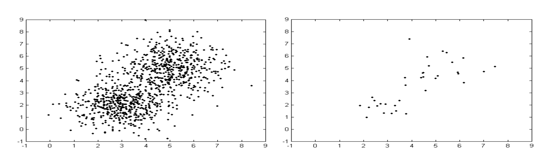
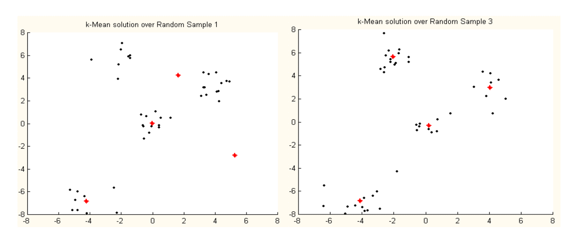
The basic heuristic is that severely subsampling the data will naturally bias the sample to representatives “near” the modes. In general, one cannot guard against the possibility of points from the tails appearing in the subsample. We have to overcome the problem that the estimate is fairly unstable due to elements of the tails appearing in the sample. Figure 1 shows data drawn from a mixture of two Gaussians (clusters) in 2-D with means at $[3,2]$ and $[5,5]$. On the left is the full data set, on the right a small subsample is shown, providing information on the modes of the joint probability density function. Each of the points on the right may be thought of as a “guess” at the possible location of a mode in the underlying distribution. The estimates are fairly varied, but they certainly exhibit “expected” behavior. Worthy of note here is that good separation between the two clusters is achieved. This observation indicates that the solutions obtained by clustering over a small subsample may provide good refined initial estimates of the true means, or centroids, in the data. However, this method often produces noisy estimates due to single small subsamples, especially in skewed distributions and high dimensions (Figure 2). This behavior is fairly common when clustering over small subsamples. In fact it is surprisingly frequent even in low dimensions using data from well-separated Gaussians[^1]. Figure 2 can also be used to illustrate the importance of the problem of having a good initial points. An initial cluster center attracting no data may remain empty (Figure 2, left), while a starting point with no empty clusters usually produces better solutions (right).

[^1]: In fact data from well-separated Gaussians in low-D are a “best-case” scenario for the behavior of a random sampling based approach. Note the idealized conditions: no noise, algorithm given the correct number of clusters $K$. With real-wold data ideal conditons are difficult to achieve, hence the behavior is expected to be worse (and indeed it is).

2.1 Clustering Clusters

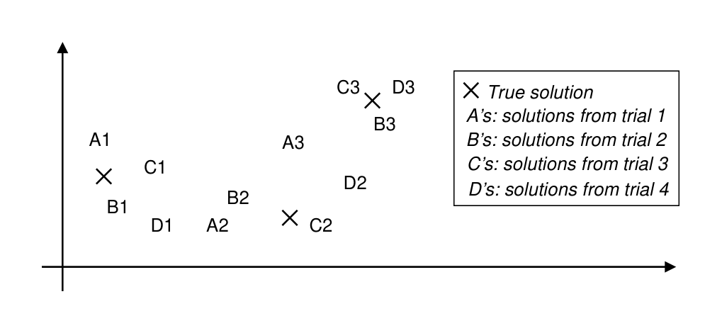
In order to overcome the problem of noisy estimates, we employ the following procedure. Multiple subsamples, say $J$, are drawn and clustered independently producing $J$ estimates of the true cluster locations. To avoid the noise associated with each of the $J$ solutions, we employ a “smoothing” procedure. However, to “best” perform this smoothing, one needs to solve the problem of grouping the $K*J$ points ($J$ solutions, each having $K$ clusters) into $K$ groups in an “optimal” fashion. Figure 3 shows 4 solutions obtained for $K=3$, $J=4$. The “true” cluster means are depicted by “X”. The A’s show the 3 points obtained from the first subsample, B’s second, C’s third, and D’s fourth. The problem then is determining that D1 is to be grouped with A1 but A2 should not be grouped with {A1, B1, C1, D1}.

2.2 The Refinement Algorithm

The refinement algorithm initially chooses $J$ small random sub-samples of the data, $S_i$, $i=1,\dots,J$. The sub-samples are clustered via K-Means with the proviso that empty clusters at termination will have their initial centers re-assigned and the sub-sample will be re-clustered. The sets $CM_i$, $i=1,\dots,J$ are these clustering solutions over the sub-samples which form the set $CM$. $CM$ is then clustered via K-Means initialized with $CM_i$ producing a solution $FM_i$. The refined initial point is then chosen as the $FM_i$ having minimal distortion over the set $CM$.

Clustering $CM$ is a smoothing over the $CM_i$ to avoid solutions “corrupted” by outliers included in the sub-sample $S_i$. The refinement algorithm takes as input: $SP$ (initial starting point), $Data$, $K$, and $J$ (number of small subsamples to be taken from $Data$):

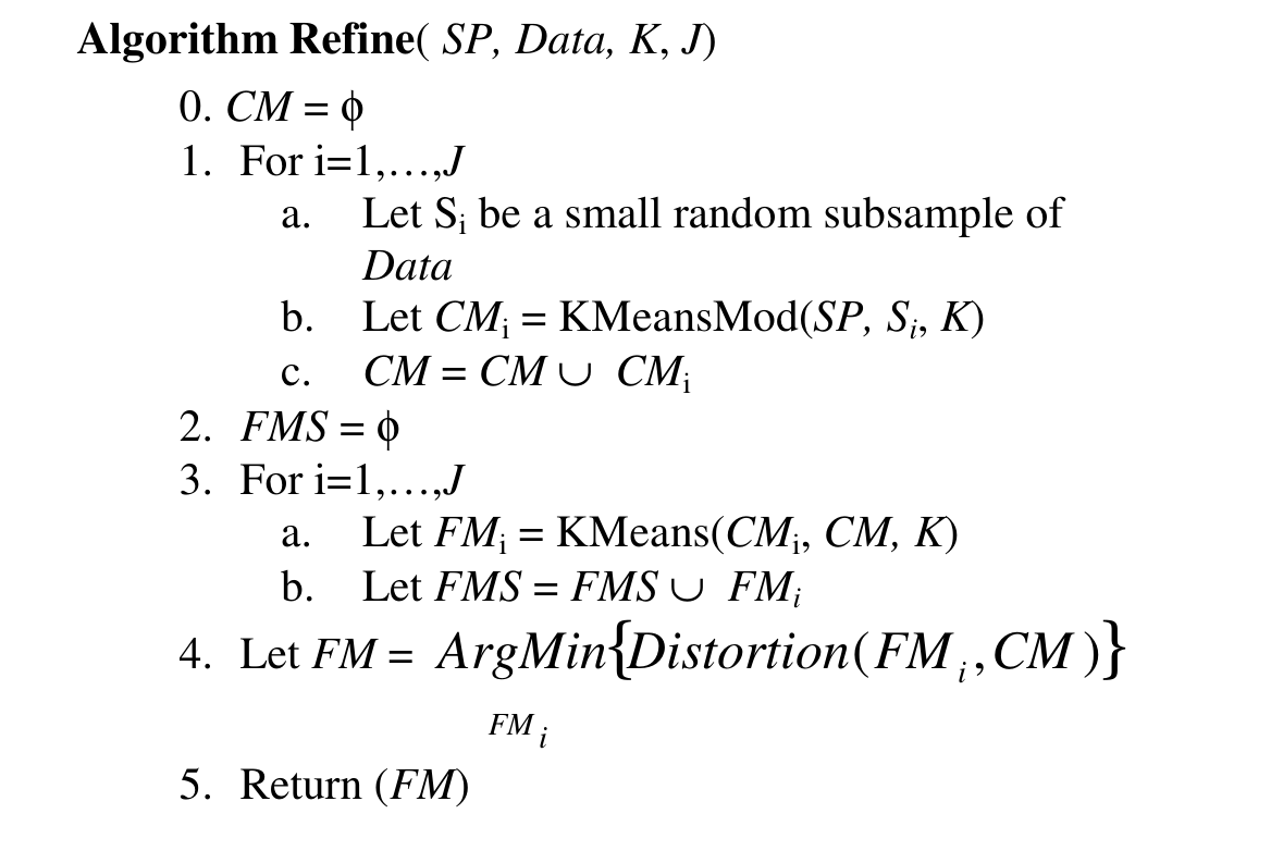
We define the following functions called by the refinement algorithm: KMeans( ), KMeansMod( ) and Distortion( ). KMeans is simply a call to the classic K-Means algorithm taking: an initial starting point, dataset and the number of clusters $K$, returning a set of $K$ $d$-dimensional vectors, the estimates of the centroids of the $K$ clusters. KmeansMod takes the same arguments as KMeans (above) and performs the same iterative procedure as classic K-Means except for the following slight modification. When classic K-Means has converged, the $K$ clusters are checked for membership. If any of the $K$ clusters have no membership (which often happens when clustering over small subsamples), the corresponding initial estimates of the empty cluster centroids are set to data elements which are farthest from their assigned cluster center, and classic K-Means is called again from these new initial centriods. The heuristic re-assignment is motivated by the following: if, at termination of K-Means, there are empty clusters then reassigning all empty clusters to points farthest from their respective centers decreases distortion most at this step. An example of clusters having zero membership is depicted in Figure 3 (left).

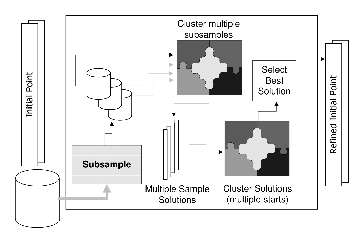
Distortion takes set of $K$ estimates of the means and the data set and computes the sum of squared distances of each data point to its nearest mean. This scalar measures the degree of fit of a set of clusters to the dataset. The K-Means algorithm terminates at a solution which is locally optimal for this distortion function [SI84]. The refinement process is illustrated in the diagram of Figure 4.

2.3 Computational Complexity and Scalability to Large Databases

The refinement algorithm is primarily intended to work on large databases. When working over small datasets (e.g. most data sets in the Irvine Repository), applying the classic K-Means algorithm from many different starting points is a feasible option. However, as database size increases (especially in dimensionality), efficient and accurate initialization becomes critical. A clustering session on a data set with many dimensions and tens of thousands or millions of records can take hours to days. In [BFR98], we present a method for scaling clustering to very large databases, specifically targeted at databases not fitting in RAM. We show that accurate clustering can be achieved with improved results over classic K-Means applied to an appropriately sized random subsample of the database [BFR98]. Scalable clustering methods obviously benefit from better initialization.

Since our method works on very small samples of the data, the initialization is fast. For example, if we use sample sizes of 1% (or less) of the full dataset size, trials over 10 samples can be run in time complexity that is less than 10% of the time needed for clustering the full database. For very large databases, the initial sample becomes negligible in size.

If, for a data set $D$, a clustering algorithm requires $\text{Iter}(D)$ iterations to cluster it, then time complexity is $|D| * \text{Iter}(D)$. A small subsample $S \subseteq D$, where $|S| \ll |D|$, typically requires significantly fewer iteration to cluster. Empirically, it is safe to expect that $\text{Iter}(S) < \text{Iter}(D)$. Hence, given a specified budget of time that a user allocates to the refinement process, we simply determine the number $J$ of subsamples to use in the refinement process. When $|D|$ is very large, and $|S|$ is a small proportion of $|D|$, refinement time is essentially negligible, even for large $J$.

Another desirable property of the refinement algorithm is that it easily scales to very large databases. The only memory requirement is to hold a small subsample in RAM. In the secondary clustering stage, only the solutions obtained from the $J$ subsamples need to be held in RAM.

Note we assume that it is possible to obtain a random sample from a large-scale database. While this sounds simple, in reality this can be a challenging task. Unless one can guarantee that the records in a database are not ordered by some property, random sampling can be as expensive as scanning the entire database (using some scheme such as reservoir sampling, e.g. [J62]). Note that in a database environment, what one thinks of as a data table (a view) may not exist as a physical table. The result of a query may involve joins, groupings, and sorts. In many cases database operations impose a special ordering on the result set, and “randomness” of the resulting database view cannot be assumed in general.

2.4 An Example

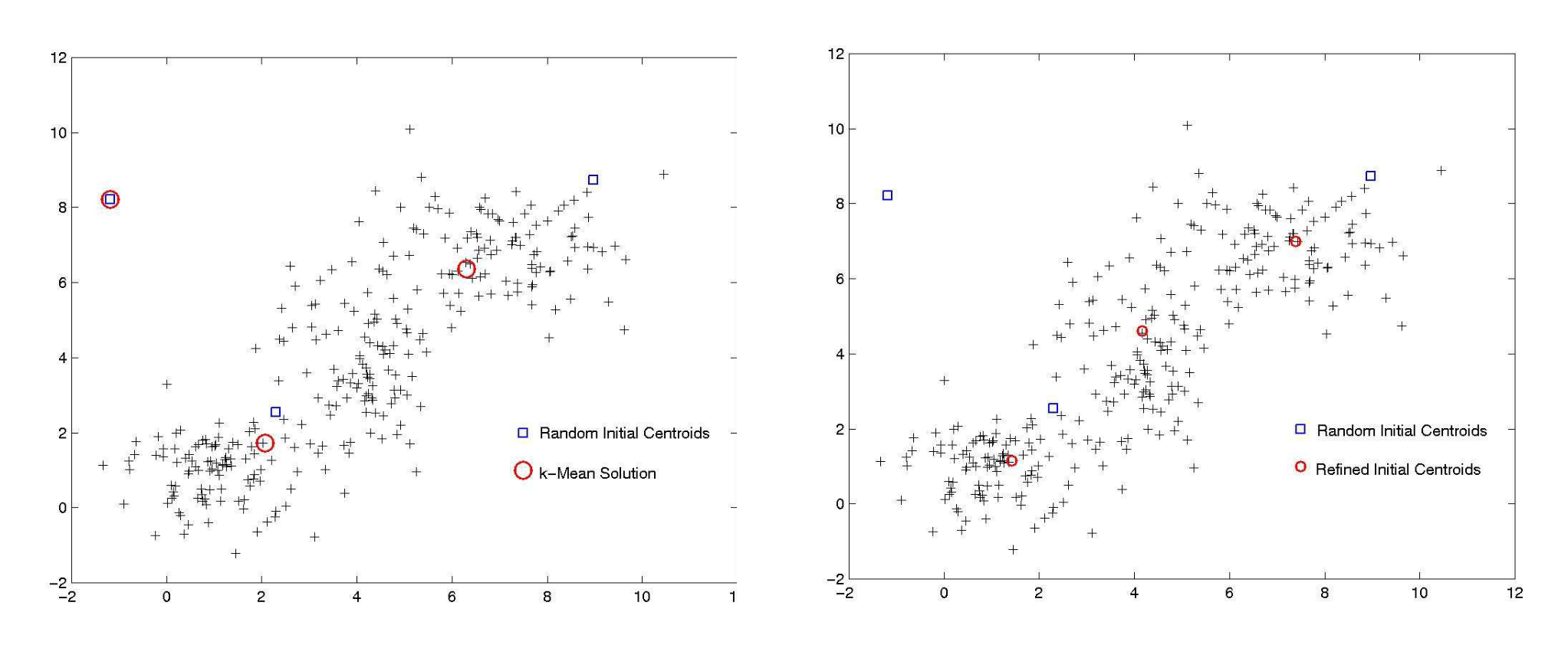
Figure 5 illustrates the sensitivity of K-Means solutions to initial conditions. Elements are sampled from three Gaussians in 2 dimensions. Note that the Gaussians in this case happen to be centered along a diagonal. The reason for this choice is that even as the dimensionality of the data goes higher, any 2 dimensional projection of the higher dimensional data will have this same form, making the data set easy for a visualization-based approach. Simply project the data to 2 dimensions, and the clusters reveal themselves. This is a rare property since, if the Gaussians are not aligned along the diagonal, any lower-dimensional projection may result in overlaps and separability in 2 dimensions is lost. The left figure shows a random starting point and the corresponding K-Means solution. The right figure shows the same initial random points and the result of the refinement procedure on this random initial point. Note that in this case the refined point is very close to the true solution. Running K-Means from the refined point converges to the true solution.

It is important to point out that this example is for illustrative purposes only. The interesting cases are high-dimensional data sets with more data items. Computational results indicate that the refinement method scales well to higher dimensions (100-D and more).

3. RESULTS ON SYNTHETIC DATA

Section Summary: Synthetic data was generated across dimensions from 2 to 100 by sampling points from 10 unevenly weighted Gaussians whose means and variances were chosen randomly. Researchers then ran standard K-Means starting from a purely random point, from a point refined over ten random subsamples, or from a point refined over one subsample, and measured how close the resulting cluster centers came to the true generating means after optimal matching. Across repeated trials the ten-subsample refinement produced solutions that were consistently nearer to the true centers than either alternative, with the advantage growing as dimensionality increased.

3.1 Data Set Description

Synthetic data was created for dimension $d = 2, 3, 4, 5, 10, 20, 40, 50$ and $100$. For a given value of $d$, data was sampled from 10 Gaussians (hence $K=10$) with elements of their mean vectors (the true means) $\mu$ sampled from a uniform distribution on $[-5,5]$. Elements of the diagonal covariance matrices $\Sigma$ were sampled from a uniform distribution on $[0.7,1.5]$. The number of data points sampled was chosen as 20 times the number of parameters estimated by K-Means. The $K=10$ Gaussians were not evenly weighted.

3.2 Experimental Methodology

The goal of this experiment is to evaluate how close the means estimated by classic K-Means are to the true Gaussian means generating the synthetic data. We compare 3 initializations:

1. No Refinement: random starting point chosen uniformly on the range of the data.
2. Refinement ($J=10$): a starting point refined from (1) using our method. The size of the random subsamples being 10% of full dataset size and the number of subsamples taken being 10.
3. Refinement ($J=1$): same as 2 but over a single random subsample of size 10%.

Once classic K-Means has computed a solution over the full dataset from any of the 3 initial points described above, the estimated means must be matched with the true Gaussian means in some optimal way prior to computing the distance between these estimated means the true Gaussian means. Let $\mu^l, l=1,\dots,K$ be the $K$ true Gaussian means and let $\bar{x}^l, l=1,\dots,K$ be the $K$ means estimated by classic K-Means over the full dataset. A “permutation” $\pi$ is determined so that the following quantity is minimized: $\sum_{l=1}^K |\mu^l - \bar{x}^{\pi(l)}|_2$. The “score” for a solution computed by classic K-Means over the full dataset is simply the above quantity divided by $K$. This is the average distance between the true Gaussian means and those estimated by K-Means over the full dataset from a given initial starting point.

3.3 Experimental Results

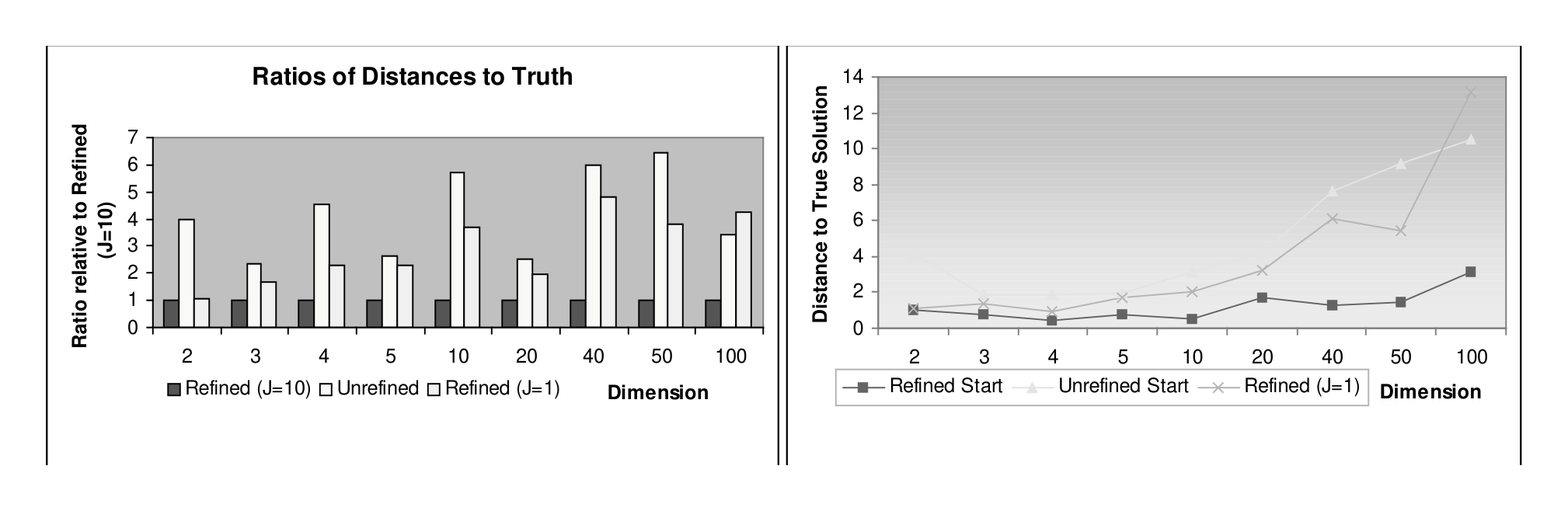
Figure 6 summarizes results averaged over 10 random initial points determined uniformly on the range of the data. Note that the K-Means solution computed from “Refined (J=10)”, is consistently nearer to the true Gaussian means generating the dataset than the K-Means solution computed from either the random initial point or the “Refined (J=1)” initial point. On the left we summarize ratios of average distance to the true Gaussian means relative to the average distance for the classic K-Mean solution computed from the refined initial point. Worthy of note in these results are the following facts:

1. For dimensions 2-50, the refinement method (Refined (J=10)) always did better than the random starting point (Unrefined) and the point refined over 1 subsample (Refined (J=1)).
2. For dimension 100, in 9 of the 10 independent trials our refinement method did better than the random starting point.
3. Refiner solutions are between 2.34 ($d=3$) and 6.44 ($d=50$) times closer to the true Gaussian means than solutions from the random initial point and between 1.09 ($d=3$) and 4.80 ($d=50$) times closer than solution computed from “Refined (J=1)” initial point.

In one run, we did slightly worse. This explains the large variance number for 100 dimensions. If we exclude that one data point, the variance drops to within range of all other dimensions. The fact that the minimum ratio occurs for datasets with small dimensionality and the maximum ratio occurs for datasets with large dimensionality indicates the utility of the refinement algorithm for large-dimensional datasets.

4. RESULTS ON REAL-WORLD DATA

Section Summary: The section explains that the refinement method for K-Means is most useful on large real-world datasets, where clustering is computationally expensive and a strong initial starting point can substantially speed convergence, since the refinement itself runs quickly on small subsamples. On smaller UCI datasets such as Image Segmentation, refined starts produced solutions with roughly 2.6 times higher information gain and 44% lower distortion than random initialization. The authors note that real-world class labels often do not match the distortion objective minimized by K-Means, but the approach still improves results across both large and modest-sized data.

We present computational results on 2 classes of publicly available “real-world” datasets. We are primarily more interested in large databases -- hundreds of dimensions and tens of thousands to millions or records. It is for these data sets that our method exhibits the greatest value. The reason is simple: a clustering session on a large database is a time-consuming affair. Hence a refined starting condition can insure that the time investment pays off.

To illustrate this, we used a large publicly available data set available from Reuters News Service. The data is described in Section 4.2. We also wanted to demonstrate the refinement procedure using data sets from the UCI Machine Learning Repository. For the most part, we found that these data sets are too easy: they are low dimensional and have a very small number of records. With a small number of records, it is feasible to perform multiple restarts efficiently. Since the sample size is small to begin with, sub-sampling for initialization is not effective. Hence most of these data sets are not of interest to us. Nevertheless, we report on our general experience with them as well as detailed experience with one of these data sets to illustrate that the method we advocate is useful when applied to smaller data sets. We emphasize, however, that our refinement procedure is best suited for large-scale data. The refinement algorithm operates over small sub-samples of the database and hence run-times needed to determine a “good” initial starting point (which speeds the convergence on the full data set) are orders of magnitude less than the total time needed for clustering in a large-scale situation.

We note that it is very likely that the cluster labeling associated with many real-world databases do not correspond to the distortion measure minimized by K-Means.

4.1 Datasets from UCI ML Repository

We evaluated our method on several Irvine data sets. First we present results on the Image Segmentation data set, then we discuss the results over the other data sets.

Image Segmentation Data Set

This data set consists of 2310 data elements in 19 dimensions. Instances are drawn randomly from a database of 7 outdoor images (brickface, sky, foliage, cement, window, path, grass). Each of the 7 images is represented by 330 instances.[^2]

[^2]: For a more detailed description of the data, see the the Irvine ML Data Repository at http://www.ics.uci.edu/~mlearn/MLRepository.html

Experimental Methodology

Random initial starting points were computed by sampling uniformly over the range of the data. We compare solutions achieved by the classic K-Means algorithm starting from: 1) random initial starting points, and 2) initial points refined by our method.

Once classic K-Means has converged, the “quality” of the solution must be determined. Unlike the case of synthetic data, we cannot measure distance to the true solution since “truth” is not known. However, we can use average class purity within each cluster as one measure of quality. The other measure, which is not dependent on a classification, is the distortion of the data given the clusters. Quality scoring methods are:

Information Gain: estimates the “amount of information” gained by clustering the database as measured by the reduction in class impurity within clusters. For a database with $L$ known classes, let $c^l$ be the number of data elements in class $l$ where $l = 1, \dots, L$. Let $m$ be the total number of data points in the database. The Total Entropy of the database is: $\text{Total Entropy} = \sum_{l=1}^L \left( \frac{c^l}{m} \right) \log \left( \frac{c^l}{m} \right)$.

Upon convergence of the classic K-Means algorithm from a given initial starting point, the Weighted Entropy is computed over the given clustering as follows: Form the $K \times L$ cluster/class matrix $C$ with the $(i, j)$-th element being the number of elements of class $j$ belonging to cluster $i$. Notice that the clustering will completely recover the assigned classes if the cluster/class matrix has a permuted identity nonzero structure. Let $CS_k$ be the size of the $k$-th cluster, then class entropy for the $k$-th cluster is given by: $\text{ClusterEntropy}(k) = \sum_{l=1}^L \left( \frac{C_{k,l}}{CS_k} \right) \log \left( \frac{C_{k,l}}{CS_k} \right)$.

The weighted entropy of the entire clustering is given by: $\text{WeightedEntropy}(K) = \sum_{k=1}^K \left( \frac{CS_k}{M} \right) \text{ClusterEntropy}(k)$.

$\text{Information Gain} = \text{Total Entropy} - \text{Weighted Entropy}(K)$.

Distortion: Given the $K$ means estimated by the classic K-Means algorithm, the distortion value that we consider is simply the sum of the $L2$ distance squared between the data items and the mean of their assigned cluster. A smaller value for the distortion measure indicates that the model parameters (i.e. means) are a better fit to the database given the K-Means assumptions are true.

Results: Image Segmentation Database

Average information gain over 10 random initial points for classic K-Mean without refining the initial point was $0.3125 \pm 0.3188$ ($\pm$ one standard deviation). Average information gain for K-Mean initialized from a refined ($J = 10$) starting point was $0.8195 \pm 0.1458$. The amount of information gained on average by the solutions computed from the refined point was 2.6222 time that of the solution computed over the random initial point.

Furthermore, on average, solutions computed from the refined initial points ($J=10$) reduced distortion by 44.41% over solutions computed from random initial points.

4.2 Other Real World Datasets

We evaluated the refinement procedure on other data sets such as Fisher’s IRIS, Star-Galaxy-Bright, etc. Because these data sets are very low dimensional and their sizes small, the majority of the results were of no interest. Clustering these data sets from random initial points and from refined initial points led to approximately equal gain in entropy and equal distortion measures in most cases. We did observe, however, that when a random starting point leads to a “bad” solution, then refinement indeed takes it to a “good” solution. So in those (admittedly rare) cases, refinement does provide expected improvement. We use the Reuters information retrieval data set to demonstrate our method on a real and difficult clustering task.

Reuters Information Retrieval Data Set

The Reuters text classification database is derived from the original Reuters-21578 data set made publicly available as part of the Reuters Corpus, through available as part of the Reuters Corpus, through Reuters, Inc., Carnegie Group and David Lewis[^3]. This data consists of 12,902 documents. Each document is a news article about some topic: e.g. earnings, commodities, acquisitions, grain, copper, etc… There are 119 categories, which belong to some 25 higher level categories (there is a hierarchy on categories). The Reuters database consists of word counts for each of the 12,902 documents. There are hundreds of thousands of words, but for purposes of our experiments we selected the 302 most frequently occurring words, hence each instance has 302 dimensions indicating the integer number of times the corresponding word occurs in the given document. Each document in the IR-Reuters database has been classified into one or more categories. We use $K=25$ for clustering purposes to reflect the 25 top-level categories. The task is then to find the best clustering given $K=25$.

[^3]: See: http://www.research.att.com/~lewis/ reuters21578/ README.txt for more details on this data set.

Reuters Results

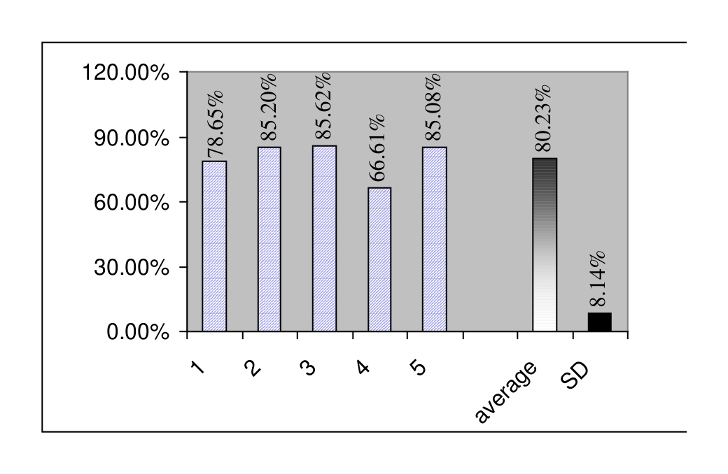
For this data set, because clustering the entire database requires a large amount of time, we chose to only evaluate results over 5 randomly chosen starting conditions. Results are shown in the chart of Figure 7. The chart shows a significant decrease in the total distortion measure. On average the distortion of a solution obtained by starting from a refined initial point was about 80% of the corresponding distortion obtained by clustering from the corresponding randomly chosen initial starting point. Since each document belongs to a category (there are 119 categories), we can also measure the quality of the achieved by any clustering by measuring the gain in information about the categories that each cluster gives (i.e. pure clusters are informative). This is done in the same manner we measure entropy for the image segmentation dataset of Section 4.1. The quality of the clusters can be measured by the average category purity in each cluster. In this case the average information gain for the clusters obtained from the refined starting point was 4.13 times higher than the information gain obtained without refining the initial points. The information gain for the refined clustering was 0.071 with a standard deviation of 0.001. While the unrefined initial points resulted in an average information gain of 0.017 with a standard deviation equal to 0.011.

5. CONCLUDING REMARKS

Section Summary: The paper describes a fast refinement method that improves starting points for clustering algorithms like K-Means by repeatedly applying the same algorithm to small data subsamples and then combining the results. This approach uses little memory, helps avoid poor solutions such as empty clusters, and leads to faster convergence with lower distortion and higher-quality groupings on both synthetic and real datasets. The same technique can be extended to other clustering methods and data types by using the target algorithm on the subsamples while still merging results with K-Means.

A fast and efficient algorithm for refining an initial starting point for a general class of clustering algorithms has been presented. The refinement algorithm operates over small subsamples of a given database, hence requiring a small proportion of the total memory needed to store the full database and making this approach very appealing for large-scale clustering problems. The procedure is motivated by the observation that subsampling can provide guidance regarding the location of the modes of the joint probability density function assumed to have generated the data. By initializing a general clustering algorithm near the modes, not only are the true clusters found more often, but it follows that the clustering algorithm will iterate fewer times prior to convergence. This is very important as the clustering methods discussed here require a full data-scan at each iteration and this may be a costly procedure in a large-scale setting.

Computational results on synthetic Gaussian data indicate that solutions computed by the K-Means algorithm from the refined initial points are superior to the random initial starting points and to a point refined over a single random subsample. Results on the small real-world Image Segmentation data set indicate that the K-Means solution from the refined points provide twice as much “information” than the solutions computed from the random initial point. Furthermore, the average distortion is decreased by 9%. Computational results on the Reuters database of newswire stories in 300 dimensions indicate a drop in distortion by about 20%. Information gain was improved by a factor of 4.13 times on this data set.

We believe that our method’s ability to obtain a substantial refinement over randomly chosen starting points is due in large part to our ability to avoid the empty clusters problem that plagues traditional K-Means. Since during refinement we reset empty clusters to far points and reiterate the K-Means algorithm, a starting point obtained from our refinement method is less likely to lead the subsequent clustering algorithm to a “bad” solution. Our intuition is confirmed by the empirical results.

The refinement method presented so far has been in the context of the K-Means algorithm. However, we note that the same method is easily be generalized to other algorithms, and even to discrete data (on which means are not defined). The generalized method and its use for initializing the EM algorithm, along with empirical results, is presented in [FRB98b]. The key insight here is that if some algorithm ClusterA is being used to cluster the data, then ClusterA is also used to cluster the subsamples. The algorithm ClusterA will produce a model. The model is essentially described by its parameters. The parameters are in a continuous space. The stage which clusters the clusters (i.e. step 3 of the algorithm Refine in Section 2.2) remains as is; i.e. we use the K-Means algorithm in this step. The reason for using K-Means is that the goal at this stage is to find the “centroid” of the models, and in this case the harsh membership assignment of K-Means is desirable.

Acknowledgements

Section Summary: The authors thank several people who supported their project in different ways. Cory Reina helped with coding, fixing problems, and running experiments on large amounts of data. Sue Dumais and Mehran Sahami supplied the Reuters dataset, and Chris Meek gave useful feedback on an early version of the work.

We thank Cory Reina for help on implementation, debugging, and running results over the large datasets; Sue Dumais and Mehran Sahami for making the Reuters data set available to us; and Chris Meek for valuable comments on an earlier draft.

References

Section Summary: This section lists academic citations for foundational and applied research on data clustering techniques, including statistical models like Gaussian mixtures, the expectation-maximization algorithm, and scalable methods for large databases. The references span classic works from the 1960s and 1970s on pattern classification and density estimation through 1990s advances in neural networks, Bayesian approaches, and knowledge discovery. They draw from fields such as biometrics, machine learning, and data mining to support both theoretical analysis and practical implementations.

[BR93] J. Banfield and A. Raftery, “Model-based gaussian and non-Gaussian Clustering”, Biometrics, vol. 49: 803-821, pp. 15-34, 1993.

[B95] C. Bishop, 1995. Neural Networks for Pattern Recognition. Oxford University Press.

[BMS97] P. S. Bradley, O. L. Mangasarian, and W. N. Street. 1997. "Clustering via Concave Minimization", in Advances in Neural Information Processing Systems 9, M. C. Mozer, M. I. Jordan, and T. Petsche (Eds.) pp 368-374, MIT Press, 1997.

[BFR98] P. S. Bradley, U. Fayyad, and C. Reina, “Scaling Clustering Algorithms to Large Databases”, To appear, Proc. 4th International Conf. on Knowledge Discovery and Data Mining (KDD-98). AAAI Press, Aug. 1998.

[CS96] P. Cheeseman and J. Stutz, “Bayesian Classification (AutoClass): Theory and Results”, in [FPSU96], pp. 153-180. MIT Press, 1996.

[DLR77] A.P. Dempster, N.M. Laird, and D.B. Rubin, “Maximum Likelihood from Incomplete Data via the EM algorithm”. Journal of the Royal Statistical Society, Series B, 39(1): 1-38, 1977.

[DH73] R.O. Duda and P.E. Hart, Pattern Classification and Scene Analysis. New York: John Wiley and Sons. 1973

[FHS96] U. Fayyad, D. Haussler, and P. Stolorz. “Mining Science Data.” Communications of the ACM 39(11), 1996.

[FPSU96] Fayyad, U., G. Piatetsky-Shapiro, P. Smyth, and R. Uthurusamy (Eds.) Advances in Knowledge Discovery and Data Mining. MIT Press, 1996.

[FRB98] U. Fayyad, C. Reina, and P. S. Bradley, “Refining Initialization of Expectation Maximization Clustering Algorithms”, To appear, Proc. 4th International Conf. on Knowledge Discovery and Data Mining (KDD-98). AAAI Press, Aug. 1998.

[F87] D. Fisher. “Knowledge Acquisition via Incremental Conceptual Clustering”. Machine Learning, 2:139-172, 1987.

[F65] E. Forgy, “Cluster analysis of multivariate data: Efficiency vs. interpretability of classifications”, Biometrics 21:768. 1965.

[F90] K. Fukunaga, Introduction to Statistical Pattern Recognition, San Diego, CA: Academic Press, 1990.

[J62] Jones, “A note on sampling from a tape file”. Communications of the ACM, vol 5, 1962.

[KR89] L. Kaufman and P. Rousseeuw, 1989. Finding Groups in Data, New York: John Wiley and Sons.

[M67] J. MacQueen, “Some methods for classification and analysis of multivariate observations. In Proceedings of the Fifth Berkeley Symposium on Mathematical Statistics and Probability. Volume I, Statistics, L. M. Le Cam and J. Neyman (Eds.). University of California Press, 1967.

[MH98] M. Meila and D. Heckerman, 1998. "An experimental comparison of several clustering methods", Microsoft Research Technical Report MSR-TR-98-06, Redmond, WA.

[NH98] R. Neal and G. Hinton, “A view of the EM algorithm that justifies incremental, sparse, and other variants'', in M. I. Jordan (Ed.), Learning in Graphical Models, Kluwer: 1998.

[R92] E. Rasmussen, “Clustering Algorithms”, in Information Retrieval Data Structures and Algorithms, Frakes and Baeza-Yates (Eds.), pp. 419-442, New Jersey: Prentice Hall, 1992.

[S92] D. W. Scott, Multivariate Density Estimation, New York: Wiley. 1992

[SI84] S. Z. Selim and M. A. Ismail, "K-Means-Type Algorithms: A Generalized Convergence Theorem and Characterization of Local Optimality." IEEE Trans. on Pattern Analysis and Machine Intelligence, Vol. PAMI-6, No. 1, 1984.

[S86] B.W. Silverman, Density Estimation for Statistics and Data Analysis, London: Chapman & Hall, 1986.

[TMCH97] B. Thiesson, C. Meek, D. Chickering, and D. Heckerman, 1997. "Learning Mixtures of Bayesian Networks", Microsoft Research Technical Report TR-97-30, Redmond, WA.

[ZRL97] T. Zhang, R. Ramakrishnan, and M. Livny. "BIRCH: A new data clustering algorithm and its applications", Data Mining and Knowledge Discovery, vol. 1, no. 2, 1997.