
Nora: Normalized Orthogonal Row Alignment for Scalable Matrix Optimizer
Jinghui Yuan$^{1*}$, Jiaxuan Zou$^{2,4*}$, Shuo Wang$^{3}$, Yong Liu$^{4}$ $^{\dagger}$, Feiping Nie$^{1}$
- School of Artificial Intelligence, Optics and Electronics (iOPEN)
Northwestern Polytechnical University. - School of Mathematics and Statistics, Xi’an Jiaotong University.
- Institute for Interdisciplinary Information Sciences, Tsinghua University.
- Gaoling School of Artificial Intelligence, Renmin University of China.
[email protected], [email protected], [email protected],[email protected], [email protected]
$^{*}$ These authors contributed equally.
$^{\dagger}$ Corresponding Author.
Abstract
Matrix-based optimizers have demonstrated immense potential in training Large Language Models (LLMs), however, designing an ideal optimizer remains a formidable challenge. A superior optimizer must satisfy three core desiderata: efficiency, achieving Muon-like preconditioning to accelerate optimization; stability, strictly adhering to the scale-invariance inherent in neural networks; and speed, minimizing computational overhead. While existing methods address these aspects to varying degrees, they often fail to unify them, either incurring prohibitive computational costs like Muon, or allowing radial jitters that compromise stability like RMNP. To bridge this gap, we propose Nora, an optimizer that rigorously satisfies all three requirements. Nora achieves training stability by explicitly stabilizing weight norms and angular velocities through row-wise momentum projection onto the row orthogonal complement of the weights. Simultaneously, by leveraging the row block diagonal dominance of the Transformer Hessian, Nora effectively approximates structured preconditioning while maintaining an optimal computational complexity of $\mathcal{O}(mn)$. Furthermore, we prove that Nora is a scalable optimizer and establish its corresponding scaling theorems. With a streamlined implementation requiring only two lines of code, our preliminary experiments validate Nora as an efficient and highly promising optimizer for large-scale training.
Executive Summary: This work addresses the challenge of optimizing large language models using matrix-based methods. While traditional vector-based optimizers like Adam overlook structural matrix properties, newer matrix optimizers such as Muon face heavy computational overhead due to iterative matrix orthogonalization. Alternative approximations, like Row-wise Momentum Normalization (RMNP), reduce this computational cost but ignore the scale-invariance of normalized neural networks. Radial momentum updates in scale-invariant layers perturb parameter magnitudes without altering functional outputs, causing unstable effective learning rates and degrading training stability. The authors set out to develop an optimizer that unifies effective preconditioning, training stability respecting scale invariance, and high execution speed.
To resolve this trade-off, the authors propose Nora, an algorithm based on normalized orthogonal row alignment. Nora operates by first projecting the accumulated momentum onto the row-wise orthogonal complement of the weight matrix, eliminating radial momentum noise and restricting updates to the tangent space. Exploiting the row-block diagonal dominance observed in Transformer second-order derivative matrices (Hessians), Nora then applies a diagonal preconditioning operator to this projected momentum. This mathematical step simplifies to simple row-wise normalization, preserving row-level perpendicularity to the weights while matching the computational complexity of element-wise operations.
The authors prove that Nora adheres to the Maximal Update Parametrization framework, which guarantees stable feature learning as model width increases when the learning rate scales inversely with the square root of the layer width. They also establish non-convex convergence guarantees, confirming that Nora reaches stationary points under standard smoothness conditions. In empirical benchmarks training LLaMA-style models at 60-million and 135-million parameter scales on the C4 dataset, Nora achieved lower validation loss and validation perplexity than Muon, Mano, and RMNP. Benchmark runtime measurements showed that row-wise normalization executes significantly faster than the Newton-Schulz iterations used in Muon, achieving over a seventy-fold speedup on large multi-layer perceptron matrices.
These findings demonstrate that optimizer designers can bypass expensive matrix iterations by leveraging specific structural properties of Transformer architectures and respecting weight-space symmetries. Nora provides a fast, stable, and theoretically supported alternative that can be implemented in two lines of matrix code without altering the underlying network architecture.
A primary qualification of the work is that the empirical evaluations were conducted on relatively small model scales up to 135 million parameters. Validating whether the observed late-stage convergence benefits and scaling laws hold for frontier-scale models with billions of parameters remains an open area for future evaluation.
1. Introduction
Section Summary: The introduction highlights limitations in existing optimizers for training large language models: methods like Adam ignore the loss landscape's structure, while matrix-based approaches such as Muon deliver strong results but incur high computational costs, and faster approximations like RMNP overlook scale invariance in neural networks, which can destabilize training through unwanted momentum effects. To overcome these trade-offs, the authors introduce Nora, which projects momentum onto directions perpendicular to the weights and applies simple row-wise normalization to achieve efficient preconditioning, training stability, and fast execution in just a few lines of code. The section also notes that Nora includes theoretical convergence guarantees, scalability analysis via the μP framework, and strong empirical results when training LLaMA models across different learning rates.
The training of Large Language Models (LLMs) relies heavily on adaptive optimizers such as Adam [1, 2]. However, such methods treat parameters as flat vectors, thereby overlooking the rich structural interactions inherent in the loss landscape [3]. Recently, matrix-based optimizers like Muon have emerged to bridge this gap, achieving state-of-the-art data efficiency through orthogonalized updates [4]. Despite its remarkable performance, Muon relies on the Newton-Schulz iteration [5], which introduces significant computational overhead of $\mathcal{O}(m^2n)$, where the weight matrix $w \in \mathbb{R}^{m \times n}$. Without loss of generality, we assume $m \le n$.
Subsequent research has sought to approximate this preprocessor. Dong et al.[6] identified the row block diagonal dominance of the Transformer Hessian, a phenomenon also noted by [7], who proposed a simplified preprocessor approximating Muon via diagonal matrices. This led to the development of RMNP (Row-wise Momentum Normalization). Although RMNP is computationally superior, it overlooks a important property of neural networks: weight space symmetry [8]. Due to the pervasive use of BatchNorm [9], RMSNorm [10] and LayerNorm [11], network representations exhibit scale invariance [12]. Radial updates—those aligning with the weight vector—do not alter the functional output [13]. However, radial momentum noise can interfere with the preprocessor's output and the direction of weight learning. Simultaneously, it silently perturbs the weight norm, leading to chaotic oscillations in the effective learning rate and ultimately undermining network training [14].
Beyond these, other classical or state-of-the-art optimizers typically suffer from one or more deficiencies: they either neglect the use of preconditioners [15, 16, 17], fail to account for the scale-invariance of neural networks [18, 19], or incur excessive computational complexity [20, 21]. In fact, many existing methods simultaneously lack several of these essential properties.
Our motivation stems from a commitment to the three core principles of optimizer design: efficiency, stability, and speed. To this end, we introduce Nora. The design of Nora relies on a simple row-wise orthogonality property: row-wise normalization preserves row-wise perpendicularity to the weight. This property enables us to unify preconditioning estimation, scale-invariance, and rapid computation. Specifically, we first project the momentum $v_t$ onto its component that is row-wise perpendicular to $w_t$ to obtain $v_t^{r\perp}$, which ensures training stability through orthogonality. Subsequently, we apply a diagonal preconditioning estimation to $v_t^{r\perp}$ to derive the update $d_t$. This step efficiently approximates the Muon-like preconditioning for enhanced efficiency, yet computationally simplifies to a mere row-wise normalization, thereby simultaneously satisfying both the speed and stability requirements.
Furthermore, leveraging the Maximal Update Parametrization ($\mu$ P) framework [22], we demonstrate that Nora is a scalable optimizer and derive its optimal learning rate scaling laws. We also provide a rigorous convergence analysis, establishing theoretical guarantees for Nora in non-convex optimization landscapes. Remarkably, the core logic of Nora can be implemented in just two lines of matrix-based code, ensuring its seamless compatibility as a plug-and-play module for any existing optimizer. We evaluate Nora by training LLaMA models [23] of various scales across a range of learning rates. Our experimental results demonstrate that Nora achieves superior performance in both convergence speed and wall-clock execution time. Our contributions are three-fold:
- We propose Nora, a novel optimizer that simultaneously achieves efficiency in preconditioning estimation, stability by respecting the scale invariance of neural networks, and high computational speed during training.
- We evaluated Nora by training LLaMA models across various learning rates. Extensive experiments demonstrate that our algorithm achieves better results in terms of both training efficiency and computational wall-clock time.
- We rigorously prove through theorems that Nora is a scalable optimizer and provide scaling criteria. We also provide rigorous convergence guarantees for Nora in non-convex optimization, demonstrating that our approach is characterized by theoretical completeness.
2. Notations
Section Summary: The paper introduces standard symbols for an optimization process, where w stands for the matrix of trainable parameters and f(w) is the loss being minimized. At each step t it tracks the parameters w_t, gradients g_t, and momentum v_t, then breaks the momentum into parts that lie parallel or perpendicular to w (either as a whole or row-by-row and column-by-column). It also defines a few common matrix operations such as extracting the diagonal, taking the transpose, forming the Kronecker product, and applying a preconditioner.
Throughout this paper, $w \in \mathbb{R}^{m \times n}$ denotes the learnable matrix parameters, and $f(w)$ denotes the loss function. Let $w_t$, $g_t$, and $v_t$ denote the parameters, gradients, and momentum at iteration $t$, respectively. The operator $\text{diag}(\cdot)$ keeps the diagonal entries of a square matrix and sets all off-diagonal entries to zero. We denote the $(i, j)$-th entry of the momentum matrix by $v_{t, ij}$ and its $i$-th row by $v_{t, i:}$. We decompose momentum into $v^{\parallel}$ and $v^{\perp}$, the components parallel and orthogonal to $w$. Similarly, $v^{r\parallel}$ and $v^{r\perp}$ denote row-wise parallel and orthogonal components, while $v^{c\parallel}$ and $v^{c\perp}$ denote the corresponding column-wise components. The symbol $\otimes$ denotes the Kronecker product. The notation $(\cdot)^T$ denotes matrix transpose, and $H^{-1}[\cdot]$ denotes the action of a preconditioning operator on a vector or matrix.
3. Related Work
Section Summary: Recent work on neural network optimization has moved beyond standard vector-based methods like AdamW to matrix-aware approaches such as Muon, which orthogonalizes gradient momentum through an iterative procedure to better account for parameter interactions, though at high computational cost. A faster alternative called row-momentum normalized preconditioning simplifies this by normalizing each row of the momentum vector independently, but this shortcut overlooks the scale-invariance property of modern networks that use normalization layers. Because such networks are unaffected by the overall magnitude of their weights, updates must remain strictly orthogonal to the current weights to avoid injecting noise into the effective learning rate and destabilizing training.
3.1 Matrix-Based Optimizers and Muon
Adaptive optimizers such as AdamW [24] treat parameters as vectors and scale gradients component-wise, thereby overlooking the intricate parameter interactions within the loss landscape $f(w)$. Matrix-based optimizers instead treat the weight $w \in \mathbb{R}^{m \times n}$, typically with $m\le n$, as a structured matrix [25]. Let $g_t = \nabla f(w_t)$, and let $v_t = \beta v_{t-1} + (1-\beta) g_t$ denote the exponential moving average of the gradient. Muon orthogonalizes this momentum and uses the update direction $d_t^{\mathrm{M}} = (v_t v_t^T)^{-\frac{1}{2}}v_t$, thereby applying a global structural preconditioner. To avoid the exact inverse square root, Muon uses the Newton–Schulz iteration $X_{k+1} = \frac{1}{2} X_k (3I - X_k^T X_k)$ from a scaled initialization $X_0 \propto v_t$. This update improves the conditioning of the search direction, but the dense matrix multiplications in the Newton–Schulz loop cost $\mathcal{O}(m^2n)$ [26], limiting scalability in large LLM layers.
3.2 Row-Momentum Normalized Preconditioning
Recent studies show that the layer-wise Hessian matrices of Transformers exhibit strong row-wise block diagonal dominance [27]. Muon can be written as applying the full-spectral preconditioner $H_{M} = (v_t v_t^T)^{\frac{1}{2}} \otimes I_n$, where $v_t$ is the momentum matrix. Row-Momentum Normalized Preconditioning (RMNP) uses the row block dominant structural prior by retaining only the diagonal blocks of the Gram matrix: $H_{R} = (\text{diag}(v_t v_t^T))^{\frac{1}{2}} \otimes I_n$. This approximation reduces matrix orthogonalization to row-wise $\ell_2$ normalization of the momentum: $H_{R}^{-1}[v_t] {i:} = \frac{v{t, i:}}{|v_{t, i:}|_{2}}$. By eliminating the Newton–Schulz loop, RMNP reduces the per-iteration complexity from $\mathcal{O}(m^2n)$ to $\mathcal{O}(mn)$. However, this algebraic simplification neglects the scale symmetry of neural networks and allows unconstrained radial updates that inject noise into the training dynamics.
3.3 Scale-invariance in Neural Networks
The widespread use of BatchNorm, RMSNorm, and LayerNorm makes scale invariance a central property of modern neural networks [28]. For scale-invariant parameters $w$, the loss satisfies $f(w) = f(\lambda w)$ for any $\lambda > 0$. This property implies that the gradient is orthogonal to the weights: $\langle \nabla f(w), w \rangle = 0$. Thus, the magnitude of $w$ is decoupled from the loss value, and learning changes the angular orientation of the parameters [29, 30]. In this setting, the radial momentum component $v^{\parallel}$ interferes with angular optimization and perturbs the weight norm. This perturbation destabilizes the effective learning rate, defined as the relative angular step size, and hinders stable training [31]. Our goal is therefore to update along directions $d_t$ satisfying $\langle d_t, w_t\rangle=0$, so that the update remains orthogonal to $w_t$.
4. Nora Optimizer
Section Summary: The Nora optimizer is designed to update neural network weights in a geometrically stable way by ensuring that every change remains strictly perpendicular to the current weight vectors, avoiding wasteful radial scaling that does not affect the loss. It achieves this through a simple row-wise orthogonalization of the momentum vector followed by row-wise normalization, which serves as an efficient preconditioner that preserves the tangent-space property while controlling the growth of weight norms. This approach draws on the row-diagonal dominance of Transformer Hessians to deliver both stability and speed with minimal extra computation compared to prior methods.
4.1 Design Concept
Modern neural networks contain many scale-invariant parameters: changing $|w_t|_F$ does not change the loss. Therefore, effective motion is angular motion rather than radial motion, a point sometimes overlooked by designers. Based on the principle of stability, the update direction should strictly reside within the tangent space of $w_t$. This approach effectively filters out meaningless radial noise while preventing oscillations in the weight norm $|w_t|$. Furthermore, tangential updates allow the learning rate schedule to maintain exclusive control over the angular velocity (i.e., the effective learning rate), since the parameter norm grows at a negligible rate and the preconditioning typically yields an update magnitude determined by the matrix dimensions $\mathbb{R}^{m \times n}$.
Existing preconditioners do not satisfy this requirement. Even when applied to tangential momentum $v_t^{\perp}$, the Muon operator produces an update $d^M_t = (v_t^{\perp}(v_t^{\perp})^T)^{-\frac{1}{2}}v_t^{\perp}$ that deviates from the tangent direction, so $\langle d^M_t, w_t \rangle \neq 0$. RMNP has the same issue: its preconditioner can destroy the orthogonality of the update to $w_t$. SSO [32] preserves this geometric property, but it relies on a computationally intensive bisection method and is too slow in practice.
Inspired by prior work on the row block diagonal dominance of the Transformer Hessian, we observe that preconditioning can be made compatible with tangential updates by considering $v_t^{r\perp}$. Here, $v_t^{r\perp}$ is obtained by orthogonalizing $v_t$ against each row of $w_t$, ensuring that $\langle v^{r\perp}{t, i:}, w{t, i:} \rangle = 0$ for every row $i$. Based on the principle of efficiency, we seek a preconditioner for $v_t^{r\perp}$. Given the row block diagonal dominance of the Transformer Hessian, it follows that $v_t^{r\perp}(v_t^{r\perp})^T$ also exhibits row-diagonal dominance. We therefore adopt the diagonal elements of $v_t^{r\perp}(v_t^{r\perp})^T$ as the preconditioner, specifically $H_N = (\text{diag}(v_t^{r\perp} (v_t^{r\perp})^T))^{\frac{1}{2}} \otimes I_n$. Consequently, the preconditioned update simplifies to $H_N^{-1}[v_t^{r\perp}] = (\text{diag}(v_t^{r\perp} (v_t^{r\perp})^T))^{-\frac{1}{2}} v_t^{r\perp}$. Through algebraic simplification, we arrive at:
$ \begin{aligned} H_N^{-1}[v_t^{r\perp}] {i:} = ((\text{diag}(v_t^{r\perp} (v_t^{r\perp})^T))^{-\frac{1}{2}} v_t^{r\perp}){i:} = \frac{v_{t, i:}^{r\perp}}{| v_{t, i:}^{r\perp} |_2} . \end{aligned}\tag{1} $
In other words, applying the preconditioner $H_N[\cdot]$ to $v_t^{r\perp}$ is mathematically equivalent to performing a simple row-wise normalization. Furthermore, the following Equation 2 leads to our long-sought objective: by preconditioning $v_t^{r\perp}$ (which is already row-orthogonal to $w_t$), we simultaneously achieve optimal efficiency while preserving the orthogonality between $v_t^{r\perp}$ and $w_t$. This ensures that the update consistently adheres to the principle of stability.
$ \begin{aligned} &\langle H_N^{-1}[v_t^{r\perp}], w_{t}\rangle=\sum_{i=1}^{m}\langle H_N^{-1}[v_t^{r\perp}] {i:}, w{t, i:}\rangle\&=\sum_{i=1}^{m}\langle \frac{1}{| v_{t, i:}^{r\perp} |2} v{t, i:}^{r\perp}, w_{t, i:}\rangle=\sum_{i=1}^{m}\frac{1}{| v_{t, i:}^{r\perp} |2}\langle v{t, i:}^{r\perp}, w_{t, i:}\rangle=\langle (H_N^{-1}[v_t^{r\perp}])^{\perp}, w_{t}\rangle=0. \end{aligned}\tag{2} $
From the perspective of Speed, Nora maintains high efficiency and stability while introducing minimal computational overhead. The additional computation consists solely of row-wise projections of $v_t$ onto the row tangent space of $w_t$, which are element-wise operations that consume virtually no additional time compared to RMNP. Furthermore, by exploiting the row block diagonal dominance of the Transformer Hessian, Nora replaces the computationally intensive Newton-Schulz (NS) iterations used in Muon with simple row-wise normalization. This effectively reduces the overall time complexity and ensures optimal training throughput.
Furthermore, updating along the direction of $(\text{diag}(v_t^{r\perp} (v_t^{r\perp})^T))^{-\frac{1}{2}} v_t^{r\perp}$ offers additional advantages. First, the discrete tangential updates ensure that the norm of each row increases only at a second-order rate. This growth is both monotonic—guaranteeing steady progression without erratic fluctuations—and gentle, remaining strictly controllable throughout training. Moreover, the row-wise orthogonality of $d_t$ relative to $w_t$ ensures a uniform growth rate across all rows of $w_t$. By upholding the geometric consistency of scale-invariant parameters, this mechanism effectively mitigates internal covariate shift and maintains the representation balance of the neural network.
It is also noteworthy that, due to the row-block diagonal dominance of the Transformer Hessian, Nora consistently performs row-wise normalization on the momentum $v_t^{r\perp}$ regardless of whether $m \le n$ or $m \ge n$. This stands in stark contrast to Muon, which restricts its Newton-Schulz iterations to the square matrix of the smaller dimension. The comprehensive procedure of the Nora algorithm is detailed in Algorithm 1. Furthermore, Table 1 presents a comparative summary of how various optimizers adhere to the three core design principles.
Require: Layer Weight $w_t \in \mathbb{R}^{m \times n}$, momentum $v_t \in \mathbb{R}^{m \times n}$, learning rate $\eta_t$ at step $t$, momentum coefficient $\beta$, and weight decay coefficient $\lambda$ (Default $\lambda$ = 0).
Initialize $v_0 \gets \mathbf{0} \in \mathbb{R}^{m \times n}, t \gets 0$.
for each step do
  $g_t \gets \nabla f(w_t)$
  $v_t \gets  \beta v_{t-1} +(1-\beta) g_t$
  $v_{t,i:}^{r\perp} \gets v_{t,i:}-\frac{\langle v_{t,i:},w_{t,i:} \rangle}{\|w_{t,i:}\|^2_2}w_{t,i:}$ // For all Row
  $d_t \gets (\text{diag}(v_t^{r\perp} (v_t^{r\perp})^T))^{-\frac{1}{2}} v_t^{r\perp}$ // Row Normalization
  $w_{t+1} \gets w_t - \eta_t  (d_t + \lambda w_t)$
end for
::: {caption="Table 1: Comparison of Optimizers Based on the Three Design Principles"}

:::
4.2 Theoretical Analysis
We now analyze Nora as a scalable optimizer and establish non-convex convergence guarantees. For a matrix $x\in\mathbb{R}^{m\times n}$, define:
$ |x|{1, 2}:=\sum{i=1}^{m}|x_{i:}|2, \qquad |x|{\infty, 2}:=\max_{1\le i\le m}|x_{i:}|_2 . $
For any matrix $w$ with nonzero rows, a matrix $z$ is row-wise perpendicular to $w$ if $\langle z_{i:}, w_{i:}\rangle=0$ for every row $i$ . The row-wise perpendicular projection is:
$ [\mathcal{P}^{r\perp}_{w}(x)] {i:} := x{i:}
\frac{\langle x_{i:}, w_{i:}\rangle}{|w_{i:}|2^2}, w{i:}.\tag{3} $
We use row-wise normalization with the convention $0/0=0$ :
$ [\operatorname{RN}(x)] {i:}:= \begin{cases} \dfrac{x{i:}}{|x_{i:}|2}, & x{i:}\neq 0, \ 0, & x_{i:}=0. \end{cases}\tag{4} $
Throughout this subsection, the scalar $m$ denotes the number of rows of $w\in\mathbb{R}^{m\times n}$, and $v_t$ denotes the momentum sequence. For $t=0, \ldots, T-1$, we analyze the core Nora update without decoupled weight decay:
$ \begin{aligned}g_t &= \nabla f(w_t;\xi_t), &v_{t+1} &= \beta v_t+(1-\beta)g_t, &v_0 &= 0, \v_{t+1}^{r\perp} &= \mathcal{P}^{r\perp}{w_t}(v{t+1}), &d_t &= \operatorname{RN}(v_{t+1}^{r\perp}), &w_{t+1} &= w_t-\eta d_t .\end{aligned}\tag{5} $
4.2.1 Scaling for Nora
In this section, we address the most fundamental engineering question in LLM training: How should the learning rate $\eta$ of Nora scale with the model width? According to the core principles of Maximal Update Parametrization ($\mu$ P), an optimal optimizer must ensure that the change in hidden layer activations, $\Delta h$, remains on the scale of $\Theta(1)$ as the network width increases ($n \to \infty$). This ensures the network neither fails to learn features due to vanishing updates nor suffers from numerical explosion. We derive the rigorous learning rate formula required for Nora to satisfy this limit through the following theorem:
########## {caption="Theorem: Nora Scaling under the Scaling Hypothesis"}
Consider a neural network layer defined by $h = wx$, where the weights $w \in \mathbb{R}^{m \times n}$ . Assume the input activation $x \in \mathbb{R}^n$ satisfies the scaling hypothesis under standard deep learning initialization: $|x|2 \le \gamma \sqrt{n}$, where $\gamma = \Theta(1)$ is a constant. Suppose the parameters are updated using Nora: $w{t+1} = w_t - \eta_t d_t$ . Then $|\Delta h_i| \le \eta_t \gamma \sqrt{n}$ . To achieve the stable feature learning limit required by $\mu$ P theory—specifically, to ensure the activation update magnitude satisfies $|\Delta h_i| = \Theta(1)$ —the learning rate $\eta_t$ for Nora must follow the width-scaling rule, $\eta_t \propto 1/\sqrt{n}$ .
The theorem provides an upper bound on the forward update, $|\Delta h_i| \le \eta_t \gamma \sqrt{n}$ . This bound ensures training stability but raises a more precise question: do Nora's projection and normalization operations substantially weaken the effective gradient components in practice, causing $\Delta h_i$ to fall significantly below $\sqrt{n}$ or even vanish? To show that Nora achieves Maximal Update Parametrization ($\mu$ P), we must evaluate the true order of $\Delta h_i$ in the high-dimensional limit $n \to \infty$ . To this end, we use the following theorem.
########## {caption="Theorem: Asymptotic Convergence"}
Consider a hidden layer $h = wx$, where $w \in \mathbb{R}^{m \times n}$ . Under the standard infinite-width random initialization hypothesis, assume the row vectors of $w$ follow $w_{i:} \sim \mathcal{N}(0, \sigma_w^2 I_n/n)$, and the components of the input activation $x \in \mathbb{R}^n$ are independent with zero mean and variance $\sigma_x^2 = \Theta(1)$ . Let the error signal backpropagated to this layer be $\delta_i = \Theta(1)$, and let the vanilla gradient without momentum be $g_{i:} = \delta_i x^\top$ . If Nora generates the update direction $d_{i:} = \operatorname{RN}(\mathcal{P}{w}^{r\perp}(g{i:}))$, then as the network width $n \to \infty$, the inner product between the update direction and the input converges in probability to $\langle d_{i:}, x \rangle \xrightarrow{p} \operatorname{sgn}(\delta_i) \sigma_x \sqrt{n}$ . Therefore, to obtain non-trivial feature learning with $\Delta h_i = \Theta(1)$, Nora must use $\eta = \eta_0/\sqrt{n}$ .
4.2.2 Convergence Analysis
We next prove non-convex convergence guarantees for Nora. Define the natural filtration as:
$ \mathcal{F}t:=\sigma(w_0, \xi_0, \ldots, \xi{t-1}). $
It is the sigma-algebra generated before sampling $\xi_t$ . Equivalently, $w_t$ and $v_t$ are $\mathcal{F}_t$ -measurable, and the conditional expectations below are taken only over the current stochastic gradient. We measure stationarity by the row-wise projected gradient:
$ \mathcal{G}t:=\mathcal{P}^{r\perp}{w_t}\bigl(\nabla f(w_t)\bigr).\tag{6} $
This is the relevant first-order signal for Nora because each row of $d_t$ is perpendicular to the corresponding row of $w_t$ . Hence its descent inner product depends only on the row-wise perpendicular component of the true gradient, not on the radial component removed by the projection. Under row-wise scale invariance, $\mathcal{G}_t$ coincides with $\nabla f(w_t)$, so the projected stationarity measure reduces to the standard first-order one.
Compared with RMNP, Nora inserts one row-wise perpendicular projection before row-wise normalization. This additional step preserves the RMNP proof structure; the main new ingredient is the non-expansiveness of $\mathcal{P}^{r\perp}_{w_t}$ in the norms used below.
########## {caption="Assumption 1: Smoothness"}
The objective $f:\mathbb{R}^{m\times n}\to\mathbb{R}$ satisfies one of the following conditions:
- (a) (Frobenius smoothness) There exists $L_F>0$ such that, for all $w, w'$,
$ |\nabla f(w)-\nabla f(w')|_F\le L_F|w-w'|_F .\tag{7} $
- (b) (Matched $(\infty, 2)$ -smoothness) There exists $L_{\infty, 2}>0$ such that, for all $w, w'$,
$ |\nabla f(w)-\nabla f(w')|{1, 2}\le L{\infty, 2}|w-w'|_{\infty, 2} .\tag{8} $
########## {caption="Theorem 2: Nora under matched $(\infty, 2)$ -smoothness"}
Suppose Assumption 1(b) hold. If Nora uses a constant step size $\eta_t=\eta$, then:
$ \frac{1}{T}\sum_{t=0}^{T-1}\mathbb{E}\bigl[|\mathcal{G}t|{1, 2}\bigr] \le \frac{\Delta}{T\eta} + 2\left[\left(1-\frac{1}{T}\right)\frac{L_{\infty, 2}\eta\beta}{1-\beta} + \frac{\sqrt{m}\sigma}{\sqrt{B}} \sqrt{\frac{1-\beta}{1+\beta}} \right] + \frac{L_{\infty, 2}\eta}{2}.\tag{9} $
Here $m$ is the row dimension of $w$ . With the choice:
$ \eta=\sqrt{\frac{(1-\beta)\Delta}{L_{\infty, 2}T}}, \qquad 1-\beta= \min\left{ \frac{\sqrt{L_{\infty, 2}\Delta}}{2\sqrt{m}\sigma\sqrt{T}}, , 1 \right},\tag{10} $
Nora reaches an $\epsilon$ -stationary point in the projected $|\cdot|_{1, 2}$ sense after:
$ T=\mathcal{O}!\left(mL_{\infty, 2}\sigma^2\Delta, \epsilon^{-4}\right)\tag{11} $
iterations.
########## {caption="Proposition 3: Frobenius-smooth counterparts"}
Under the same conditions of Theorem 2, if Nora uses a constant step size $\eta_t=\eta$, then:
$ \frac{1}{T}\sum_{t=0}^{T-1}\mathbb{E}\bigl[|\mathcal{G}_t|_F\bigr] \le \frac{\Delta}{T\eta} + (\sqrt{m}+1)\left[\left(1-\frac{1}{T}\right)\frac{L_F\eta\sqrt{m}\beta}{1-\beta} + \frac{\sigma}{\sqrt{B}} \sqrt{\frac{1-\beta}{1+\beta}} \right] + \frac{L_F\eta m}{2}.\tag{12} $
The corresponding projected $|\cdot|_{1, 2}$ bound is:
$ \frac{1}{T}\sum_{t=0}^{T-1}\mathbb{E}\bigl[|\mathcal{G}t|{1, 2}\bigr] \le \frac{\Delta}{T\eta} + 2\left[\left(1-\frac{1}{T}\right)\frac{L_F\eta m\beta}{1-\beta} + \frac{\sqrt{m}\sigma}{\sqrt{B}} \sqrt{\frac{1-\beta}{1+\beta}} \right] + \frac{L_F\eta m}{2}.\tag{13} $
Consequently, Nora reaches an $\epsilon$ -stationary point in either projected measure after:
$ T=\mathcal{O}!\left(m^2L_F\sigma^2\Delta, \epsilon^{-4}\right)\tag{14} $
iterations.
########## {caption="Corollary 4: Standard first-order stationarity under row-wise scale invariance"}
Assume, in addition, that $f$ is row-wise scale invariant:
$ f(Dw)=f(w), \qquad \forall w\in\mathbb{R}^{m\times n}, \ \forall D\succ 0\ \text{diagonal}.\tag{15} $
Then $\nabla f(w_t)$ is row-wise perpendicular to $w_t$ for all $t$, i.e.,
$ \mathcal{P}^{r\perp}_{w_t}\bigl(\nabla f(w_t)\bigr)=\nabla f(w_t).\tag{16} $
Therefore, Theorem 2 and Proposition 3 hold with $\mathcal{G}_t$ replaced by $\nabla f(w_t)$ .
Proof sketch.
The proof follows the RMNP descent argument and adds one projection lemma: for fixed $w_t$, the row-wise perpendicular projector $\mathcal{P}^{r\perp}{w_t}$ is non-expansive in $|\cdot|F$, $|\cdot|{1, 2}$, and $|\cdot|{\infty, 2}$ . Because each row of $d_t$ is perpendicular to the corresponding row of $w_t$,
$ \langle \nabla f(w_t), d_t\rangle = \left\langle \mathcal{P}^{r\perp}_{w_t}(\nabla f(w_t)), d_t\right\rangle = \langle \mathcal{G}_t, d_t\rangle.\tag{17} $
Define the projected momentum tracking error as:
$ e_t:=v_{t+1}^{r\perp}-\mathcal{G}_t . $
The row-normalization identities give:
$ \langle \mathcal{G}t, d_t\rangle \ge |\mathcal{G}t|{1, 2}-2|e_t|{1, 2}, \qquad \langle \mathcal{G}_t, d_t\rangle \ge |\mathcal{G}_t|_F-(\sqrt{m}+1)|e_t|_F.\tag{18} $
Combining these inequalities with smoothness-based descent and the standard momentum recursion yields the stated bounds. Full proofs and standard assumptions are deferred to Appendix A.
4.3 Compared with Mano
In this section, we delineate the distinctions between Mano [34] and Nora. Mano alternates between row-wise and column-wise perpendicular projections, followed by normalization. Specifically, Mano accumulates momentum $v_t$ in the standard manner. During odd iterations, it removes the row-wise radial component to obtain $v_t^{r\perp}$ and applies row normalization: $d_t = \text{RN}(v_t^{r\perp})$. During even iterations, it removes the column-wise radial component to obtain $v_t^{c\perp}$ and applies column normalization: $d_t = \text{CN}(v_t^{c\perp})$.
The design philosophy of Nora diverges significantly from that of Mano. Nora originates from the properties expected by the optimizer itself, while Mano comes from Riemannian optimization [35, 36, 37]. In practical implementation, Nora is more streamlined as it eliminates the need to track iteration parity (odd vs. even steps). More importantly, Nora is explicitly designed to leverage the row block diagonal dominance characteristic of the Transformer Hessian. By removing the heuristic column-wise orthogonal projection and normalization used in Mano, Nora demonstrates superior properties in ablation studies. These empirical results suggest that the row block diagonal dominance of the Transformer Hessian is a critical structural prior that must be prioritized.
5. Experiments
Section Summary: In experiments training LLaMA-style language models at 60M and 135M scales, Nora was compared against Muon, Mano, and RMNP using identical data, schedules, and settings, with only the core optimizer rules differing. Nora achieved the lowest validation loss and perplexity, particularly at the larger scale where it showed stronger late-training gains, and it did so without weight decay. Separate tests also showed that its row-normalization step runs far faster than the orthogonalization methods in competing optimizers, often by an order of magnitude or more on typical matrix sizes.
We evaluate Nora on autoregressive language modeling with LLaMA-style Transformer models at two scales: 60M and 135M parameters. We compare Nora with three matrix-based optimizers, Muon, Mano, and RMNP, under the same data pipeline, tokenizer, context length, global batch size, learning-rate schedule, precision, evaluation cadence, and checkpointing cadence. Detailed model and training configurations are deferred to Appendix B.
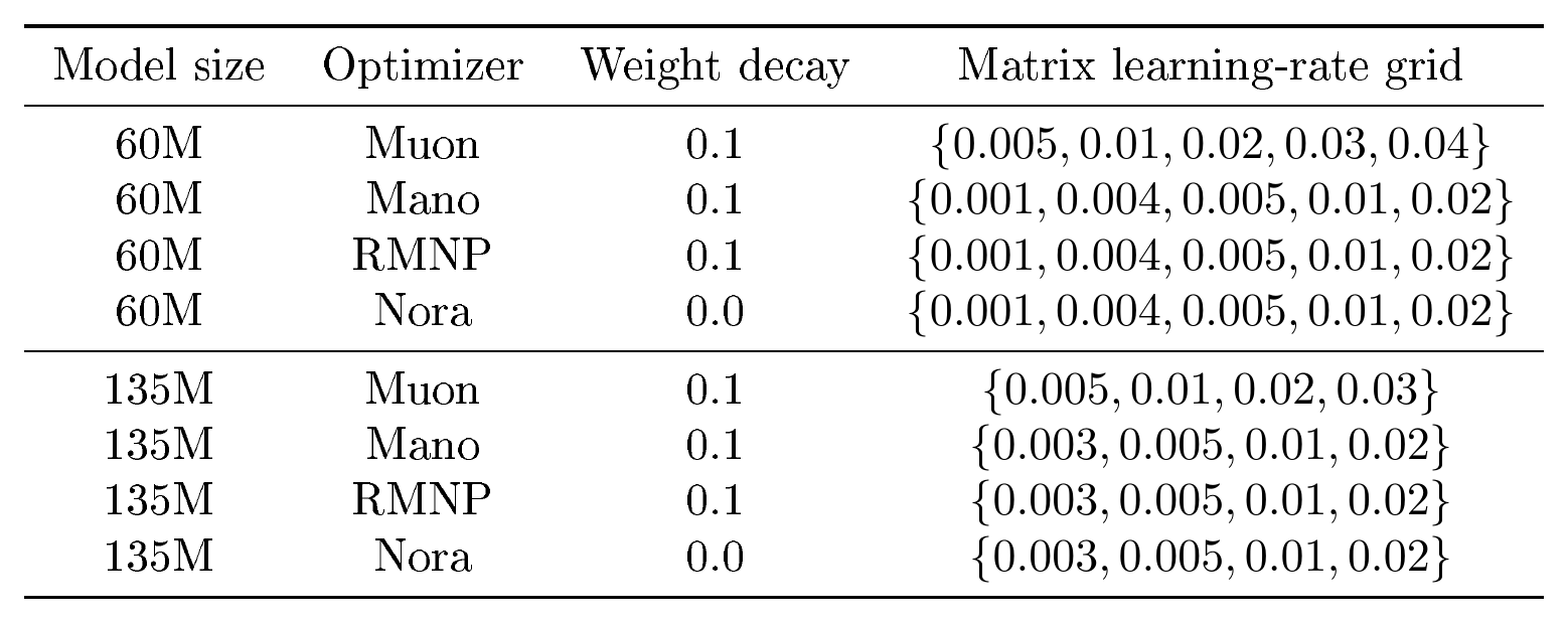
The compared optimizers differ only in the optimizer rule, the matrix learning-rate sweep grid, and weight decay. For all non-matrix parameter groups, we use the same auxiliary Adam setting within each model size. For matrix-shaped parameters, we tune the matrix learning rate over optimizer-specific grids and select the best run by validation loss. Muon uses a slightly different sweep range from the other matrix optimizers because it is more sensitive to large matrix learning rates in our preliminary runs. The full sweep grids are listed in Appendix B. Importantly, Nora uses weight decay $0$ in all runs, whereas Muon, Mano, and RMNP use weight decay $0.1$. We treat this as part of Nora's optimizer configuration and report it explicitly in all result tables.
5.1 Best Results from Different Optimizers
Table 2 reports the main language-modeling results. For each optimizer and model size, we report the matrix learning rate selected from the sweep, the validation loss at the selected setting, and validation perplexity. This format separates peak validation performance from the final checkpoint quality.
::: {caption="Table 2: Main language-modeling results. For each optimizer and model size, the matrix learning rate is selected by validation loss over the sweep grid in Appendix B. Lower validation loss and perplexity are better. Best results are shown in bold."}

:::
::: {caption="Table 3: Comparison of Mano and Nora (Model: 135M, Weight decay=0)"}

:::
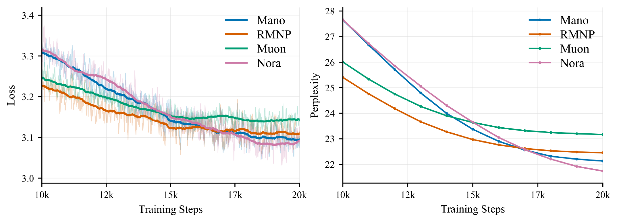
Figure 1 shows the 135M training dynamics from 10k to 20k steps. RMNP has the strongest early-stage loss and perplexity, while Muon improves more slowly and plateaus at a higher value. Mano and Nora start from higher loss and perplexity, but both continue to improve after 15k steps. Nora shows the clearest late-stage improvement: it overtakes the other methods near the end of training and reaches the lowest final loss and perplexity. This indicates that Nora uses the same training budget more efficiently, achieving better optimization quality without requiring additional training steps. This trend is consistent with Table 2, where Nora achieves the best 135M validation loss and perplexity among the compared optimizers.
5.2 Runtime Comparison
We also compare the cost of row normalization with Newton–Schulz orthogonalization on representative matrix shapes from LLaMA-style models. The benchmark uses CUDA with bfloat16 precision, 20 warmup iterations, and 200 measured iterations. Newton–Schulz uses five iterations. As shown in Table 4, row normalization is consistently cheaper than Newton–Schulz. The gap is already about one order of magnitude for small and medium matrices, and becomes much larger for the 1B-scale MLP matrices, where Newton–Schulz is more than 70 times slower. This highlights the substantial speed advantage of row normalization in practical training settings. Results support the practical motivation for replacing matrix-level orthogonalization with a row-wise normalization step.
: Table 4: Runtime comparison between row normalization and five-step Newton–Schulz orthogonalization on representative LLaMA-style matrix shapes. Times are mean kernel runtimes in milliseconds under CUDA and bfloat16 precision.
| Model scale | Matrix shape | Representative layer | Row normalization (ms) | NS(5) (ms) | NS / row-norm |
|---|---|---|---|---|---|
| 60M | 512 × 512 | attention: hidden × hidden | 0.0689 | 0.6554 | 9.52 × |
| 60M | 1376 × 512 | MLP: intermediate × hidden | 0.0682 | 0.6853 | 10.05 × |
| 60M | 512 × 1376 | MLP: hidden × intermediate | 0.0688 | 0.6623 | 9.63 × |
| 135M | 768 × 768 | attention: hidden × hidden | 0.0686 | 0.6520 | 9.50 × |
| 135M | 2048 × 768 | MLP: intermediate × hidden | 0.0692 | 0.6871 | 9.93 × |
| 135M | 768 × 2048 | MLP: hidden × intermediate | 0.0691 | 0.6534 | 9.46 × |
| 350M | 1024 × 1024 | attention: hidden × hidden | 0.0674 | 0.6397 | 9.49 × |
| 350M | 2816 × 1024 | MLP: intermediate × hidden | 0.0687 | 0.8625 | 12.56 × |
| 350M | 1024 × 2816 | MLP: hidden × intermediate | 0.0675 | 0.6941 | 10.28 × |
| 1B | 2048 × 2048 | attention: hidden × hidden | 0.0684 | 2.0552 | 30.06 × |
| 1B | 5461 × 2048 | MLP: intermediate × hidden | 0.0985 | 6.9985 | 71.02 × |
| 1B | 2048 × 5461 | MLP: hidden × intermediate | 0.1084 | 7.9678 | 73.51 × |
5.3 Ablation Experiment between Nora and Mano
To verify that row-normalization indeed captures the row-diagonal dominance inherent in the Transformer Hessian, we conducted an ablation study. Given that Nora and Mano share similar algorithmic frameworks, it is crucial to distinguish their structural advantages from hyperparameter effects. While the previous experiments utilized Mano’s recommended $\text{weight decay}=0.1$ against Nora’s default $\text{weight decay}=0$, we eliminated this discrepancy in the ablation study by setting Mano’s $\text{weight decay}$ to $0$. As shown in Table 3, the results demonstrate that Nora’s superiority stems from its intrinsic algorithmic architecture rather than an advantage gained from weight decay settings.
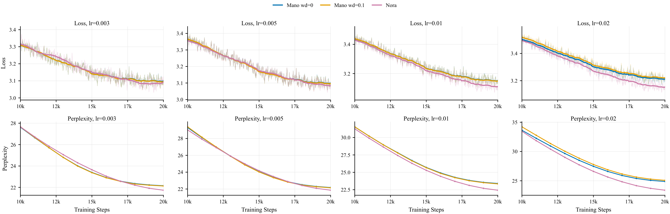
Furthermore, Figure 2 illustrates the perplexity and loss decay curves for both Mano and Nora at the 135M model scale, under configurations of $\text{weight decay}=0$ and $\text{weight decay}=0.1$. It is evident that Nora consistently outperforms Mano across all settings. For a comprehensive overview, all remaining experimental results and corresponding convergence curves are provided in Appendix B, where we focus on the sensitivity of hyper-parameters and stability of our proposed optimizer. \
6. Conclusion
Section Summary: Researchers have created a new training method called Nora for large language models that focuses on adjusting the angles of the model's internal connections rather than their overall sizes. This approach keeps training stable and efficient by applying simple row-by-row adjustments that build on existing techniques while avoiding unnecessary complications. In tests with LLaMA-style models, Nora delivered better accuracy and ran faster than comparable methods, pointing to a practical way to improve how future AI systems are trained.
We introduce Nora, a normalized orthogonal row-alignment optimizer for scalable LLM training. Nora is motivated by the geometry of scale-invariant neural networks, where effective learning should mainly occur along angular rather than radial directions. By projecting momentum onto the row-wise orthogonal complement of the weights and applying row-wise normalization, Nora preserves stable scale-invariant dynamics while retaining efficient Muon-like preconditioning under the row-diagonal structure of Transformer Hessians. We further establish Nora's scalability through $\mu$ P-based width-scaling analysis and provide non-convex convergence guarantees. Experiments on LLaMA-style models show that Nora achieves the best validation loss and perplexity among the compared matrix-based optimizers, while its row-wise normalization brings a clear speed advantage over Newton–Schulz orthogonalization. Overall, Nora demonstrates that efficiency, stability, and speed can be unified through a simple row-wise geometric principle, offering a practical and principled direction for scalable optimizer design.
normalem
Appendix
Section Summary: The appendix presents detailed mathematical proofs for two theorems on Nora, a row-wise normalization method for updating neural network weights during training. It shows that under assumptions about input scaling and random initialization in wide networks, the change in layer activations stays well-behaved only if the learning rate shrinks proportionally to one over the square root of the layer width. Additional preliminary definitions establish the notation needed for further convergence results involving momentum and projections.
A. Proof of Theorem
A.1 Proof of Theorem 4.1
Theorem 4.1 (Nora Scaling under the Scaling Hypothesis) Consider a neural network layer defined by $h = wx$, where the weights $w \in \mathbb{R}^{m \times n}$. Assume the input activation $x \in \mathbb{R}^n$ satisfies the scaling hypothesis under standard deep learning initialization: $|x|2 \le \gamma \sqrt{n}$, where $\gamma = \Theta(1)$ is a constant. Suppose Nora updates the parameters by $w{t+1} = w_t - \eta_t d_t$. Then $|\Delta h_i| \le \eta_t \gamma \sqrt{n}$. To achieve the stable feature learning limit required by $\mu$ P theory—specifically, to ensure the activation update magnitude satisfies $|\Delta h_i| = \Theta(1)$, the learning rate $\eta_t$ for Nora must follow the width-scaling rule, $\eta_t \propto \frac{1}{\sqrt{n}}$.
Proof: For any output neuron $i$, the change in the hidden activation $\Delta h_i$ during the forward pass is:
$ \Delta h_i = (w_{t+1, i:} - w_{t, i:}) x = -\eta_t \langle d_{t, i:}, x \rangle\tag{19} $
By taking the absolute value and applying the Cauchy-Schwarz inequality, we obtain:
$ |\Delta h_i| = \eta_t |\langle (d_t){i:}, x \rangle| \le \eta_t |(d_t){i:}|_2 |x|_2\tag{20} $
Nora's row-wise normalization strictly ensures $|(d_t)_{i:}|_2 \le 1$. Combined with the input assumption $|x|_2 \le \gamma \sqrt{n}$, substituting these into the inequality yields a rigorous upper bound for the forward update:
$ |\Delta h_i| \le \eta_t \cdot 1 \cdot \gamma \sqrt{n} = \eta_t \gamma \sqrt{n}\tag{21} $
To ensure that the feature update magnitude $|\Delta h_i|$ neither diverges nor vanishes as $n \to \infty$ (i.e., satisfies the Maximal Update condition $|\Delta h_i| = \Theta(1)$), we require the upper bound $\eta_t \gamma \sqrt{n}$ to also be of order $\Theta(1)$. Given that $\gamma$ is a constant, this necessarily implies $\eta_t = \frac{c}{\sqrt{n}}$, where $c$ is a constant independent of $n$. This completes the proof.
A.2 Proof of Theorem 4.2
Theorem 4.2 (symptotic Convergence)) Consider a hidden layer $h = wx$, where $w \in \mathbb{R}^{m \times n}$. Under the standard infinite-width random initialization hypothesis, assume the row vectors of $w$ follow $w_{i:} \sim \mathcal{N}(0, \frac{\sigma_w^2}{n} I_n)$, and the components of the input activation $x \in \mathbb{R}^n$ are independent with zero mean and variance $\sigma_x^2 = \Theta(1)$. Let the error signal backpropagated to this layer be $\delta_i = \Theta(1)$, and the vanilla gradient (without momentum) be $g_{i:} = \delta_i x^\top$. If Nora is applied to generate the update direction $d_{i:} = \text{RN}(\mathcal{P}{w}^{r\perp}(g{i:}))$, then as the network width $n \to \infty$, the inner product between the update direction and the input converges in probability to $\langle d_{i:}, x \rangle \xrightarrow{p} \text{sgn}(\delta_i) \sigma_x \sqrt{n}$. To achieve non-trivial feature learning such that $\Delta h_i = \Theta(1)$ as $n \to \infty$, the Nora learning rate must scale as $\eta = \frac{\eta_0}{\sqrt{n}}$.
Proof: For output neuron $i$, Nora first removes the row-wise radial component of the gradient. Writing row vectors as columns inside inner products, this gives:
$ u_{i:} = \delta_i x - \frac{\delta_i \langle x, w_{i:} \rangle}{|w_{i:}|2^2} w{i:}.\tag{22} $
We now compute the high-dimensional orders. Since $x_j$ has variance $\sigma_x^2$ and $w_{i, j}$ has variance $\sigma_w^2/n$, the weak law of large numbers gives:
$ |x|_2^2 \xrightarrow{p} n \sigma_x^2 \implies |x|_2 = \sigma_x \sqrt{n} + o_p(\sqrt{n}).\tag{23} $
Similarly:
$ |w_{i:}|_2^2 \xrightarrow{p} \sigma_w^2 = \Theta(1).\tag{24} $
Because $x$ and $w$ are independent and centered, $\langle x, w_{i:} \rangle$ is a sum of $n$ independent products with total variance $\sigma_x^2\sigma_w^2$. The central limit theorem gives:
$ \langle x, w_{i:} \rangle \xrightarrow{d} \mathcal{N}(0, \sigma_x^2 \sigma_w^2) = \mathcal{O}_p(1).\tag{25} $
Let $r_{i:}$ denote the radial component removed by the projection. Its Euclidean norm satisfies:
$ |r_{i:}|2 = \left| \frac{\delta_i \langle x, w{i:} \rangle}{|w_{i:}|2^2} \right| |w{i:}|_2 = \frac{|\delta_i| |\mathcal{O}_p(1)|}{\sigma_w^2} \sigma_w = \mathcal{O}_p(1).\tag{26} $
The primary gradient term $\delta_i x$ has norm $\Theta(\sqrt{n})$, while the removed radial component is $\mathcal{O}_p(1)$. Hence the projected vector satisfies:
$ |u_{i:}|2 = |\delta_i x - r{i:}|_2 = |\delta_i| |x|_2 + \mathcal{O}_p(1) = |\delta_i| \sigma_x \sqrt{n} (1 + o_p(1)).\tag{27} $
Row-wise normalization gives:
$ d_{i:} = \frac{u_{i:}}{|u_{i:}|2} = \frac{\delta_i x - r{i:}}{|\delta_i| \sigma_x \sqrt{n} (1 + o_p(1))}.\tag{28} $
The forward update depends on the inner product:
$ \langle d_{i:}, x \rangle = \frac{\delta_i \langle x, x \rangle - \langle r_{i:}, x \rangle}{|\delta_i| \sigma_x \sqrt{n} (1 + o_p(1))}.\tag{29} $
Since $\langle x, x \rangle = n \sigma_x^2 + o_p(n)$ and $|\langle r_{i:}, x \rangle| \le |r_{i:}|_2 |x|_2 = \mathcal{O}_p(\sqrt{n})$,
$ \langle d_{i:}, x \rangle = \frac{\delta_i n \sigma_x^2 - \mathcal{O}_p(\sqrt{n})}{|\delta_i| \sigma_x \sqrt{n} (1 + o_p(1))} = \text{sgn}(\delta_i) \sigma_x \sqrt{n} + o_p(\sqrt{n}).\tag{30} $
Thus $\langle d_{i:}, x \rangle \xrightarrow{p} \text{sgn}(\delta_i) \sigma_x \sqrt{n}$ holds. The actual forward update is $\Delta h_i = -\eta \langle d_{i:}, x \rangle = \mp \eta \sigma_x \sqrt{n}$. To achieve $\Delta h_i = \Theta(1)$ for non-trivial feature learning, it is necessary that $\eta = \Theta(n^{-1/2})$.
A.3 Preliminaries for Theorem 4.7–Corollary 4.9
A.3.1 Setup
For the convergence analysis, let $m$ denote the number of rows in $w\in\mathbb{R}^{m\times n}$ . We reserve $v_t$ for the momentum sequence. For any matrix $w$ with nonzero rows, define the row-wise perpendicular projection:
$ [\mathcal{P}^{r\perp}_{w}(x)] {i:} := x{i:}
\frac{\langle x_{i:}, w_{i:}\rangle}{|w_{i:}|2^2}, w{i:}.\tag{31} $
This projection removes the row-wise radial component: $\langle [\mathcal{P}^{r\perp}{w}(x)] {i:}, w{i:}\rangle=0$ for every row $i$ . Equivalently, a matrix $z$ is row-wise perpendicular to $w$ when $\langle z{i:}, w_{i:}\rangle=0$ for all $i$ .
For $t=0, \ldots, T-1$, Nora is indexed as:
$ g_t=\nabla f(w_t;\xi_t), \qquad v_{t+1}=\beta v_t+(1-\beta)g_t, \qquad v_0=0,\tag{32} $
$ v_{t+1}^{r\perp}:=\mathcal{P}^{r\perp}{w_t}(v{t+1}), \qquad d_t=\operatorname{RN}\bigl(v_{t+1}^{r\perp}\bigr), \qquad w_{t+1}=w_t-\eta d_t.\tag{33} $
Thus $d_t$ is the row-wise normalization of the component of the momentum that is row-wise perpendicular to $w_t$ . We use the convention $0/0=0$ in $\operatorname{RN}$, applied row-wise:
$ [\operatorname{RN}(x)] {i:} = \begin{cases} \dfrac{x{i:}}{|x_{i:}|2}, & x{i:}\neq 0, \ 0, & x_{i:}=0. \end{cases}\tag{34} $
For a matrix $x\in\mathbb{R}^{m\times n}$, define:
$ |x|{1, 2}:=\sum{i=1}^{m}|x_{i:}|2, \qquad |x|{\infty, 2}:=\max_{1\le i\le m}|x_{i:}|_2.\tag{35} $
We also define the natural filtration:
$ \mathcal{F}t:=\sigma(w_0, \xi_0, \ldots, \xi{t-1}),\tag{36} $
so that $w_t$ is $\mathcal{F}_t$ -measurable and $g_t$ is sampled conditionally on $\mathcal{F}_t$ . Finally, define the projected gradient and momentum-tracking errors:
$ \mathcal{G}t:=\mathcal{P}^{r\perp}{w_t}\bigl(\nabla f(w_t)\bigr), \qquad e_t:=v_{t+1}-\nabla f(w_t), \qquad \bar{e}t:=v{t+1}^{r\perp}-\mathcal{G}t=\mathcal{P}^{r\perp}{w_t}(e_t).\tag{37} $
The projected gradient $\mathcal{G}_t$ is the relevant stationarity measure because Nora uses directions that are row-wise perpendicular to $w_t$ . Therefore radial components of $\nabla f(w_t)$ do not contribute to the descent inner product with $d_t$ .
A.3.2 Auxiliary Lemmas
########## {caption="Lemma 5: Row-wise projection is non-expansive"}
For any $w\in\mathbb{R}^{m\times n}$ with nonzero rows and any $x\in\mathbb{R}^{m\times n}$,
$ |\mathcal{P}^{r\perp}{w}(x)|F\le |x|F, \qquad |\mathcal{P}^{r\perp}{w}(x)|{1, 2}\le |x|{1, 2}, \qquad |\mathcal{P}^{r\perp}{w}(x)|{\infty, 2}\le |x|_{\infty, 2}.\tag{38} $
Proof: For each row $i$, let
$ P_i:=I_n-\frac{w_{i:}^{\top}w_{i:}}{|w_{i:}|_2^2}.\tag{39} $
Then $[\mathcal{P}^{r\perp}_{w}(x)] {i:}=x{i:}P_i$ . Since $P_i$ is an orthogonal projector on $\mathbb{R}^n$,
$ |x_{i:}P_i|2\le |x{i:}|_2.\tag{40} $
Summing over rows gives the Frobenius and $|\cdot|{1, 2}$ bounds, while taking the maximum over rows gives the $|\cdot|{\infty, 2}$ bound.
########## {caption="Lemma 6: Basic geometry of Nora"}
Let $z=\mathcal{P}^{r\perp}_{w}(x)$ and $d=\operatorname{RN}(z)$ . Then:
- $\langle d_{i:}, w_{i:}\rangle=0$ for every row $i$ ;
- $|d|_F\le \sqrt{m}$ ;
- $|d|_{\infty, 2}\le 1$ ;
- $\langle z, d\rangle = |z|_{1, 2}$ ;
- $\langle z, d\rangle \ge |z|_F$ .
Proof: Each row $z_{i:}$ is orthogonal to $w_{i:}$ . Every nonzero row of $d$ is a scalar multiple of $z_{i:}$, so it is also orthogonal to $w_{i:}$ . Thus $d$ is row-wise perpendicular to $w$ .
For every row, $|d_{i:}|_2\le 1$ . Thus:
$ |d|F^2=\sum{i=1}^{m}|d_{i:}|2^2\le m, \qquad |d|{\infty, 2}=\max_i |d_{i:}|_2\le 1.\tag{41} $
Moreover,
$ \langle z, d\rangle = \sum_{i=1}^{m}\left\langle z_{i:}, \frac{z_{i:}}{|z_{i:}|2}\right\rangle = \sum{i=1}^{m}|z_{i:}|2 = |z|{1, 2}.\tag{42} $
Finally,
$ |z|{1, 2}=\sum_i |z{i:}|2 \ge \left(\sum_i |z{i:}|_2^2\right)^{1/2} = |z|_F,\tag{43} $
which gives $\langle z, d\rangle\ge |z|_F$ .
########## {caption="Lemma 7: Descent under Frobenius smoothness"}
Under Assumption 1(a), for every $t$,
$ f(w_t)-f(w_{t+1}) \ge \eta\langle \nabla f(w_t), d_t\rangle
\frac{L_F\eta^2 m}{2}.\tag{44} $
Proof: Let $\Delta_t:=w_{t+1}-w_t$ . By the fundamental theorem of calculus,
$ f(w_t+\Delta_t)-f(w_t) = \int_0^1 \langle \nabla f(w_t+s\Delta_t), \Delta_t\rangle, ds.\tag{45} $
Subtracting $\langle\nabla f(w_t), \Delta_t\rangle$ and applying Cauchy–Schwarz gives:
$ \begin{aligned} f(w_t+\Delta_t)-f(w_t)-\langle\nabla f(w_t), \Delta_t\rangle &= \int_0^1 \langle \nabla f(w_t+s\Delta_t)-\nabla f(w_t), \Delta_t\rangle, ds \ &\le \int_0^1 |\nabla f(w_t+s\Delta_t)-\nabla f(w_t)|_F, |\Delta_t|_F, ds . \end{aligned} $
Assumption 1(a) implies:
$ |\nabla f(w_t+s\Delta_t)-\nabla f(w_t)|_F \le L_Fs|\Delta_t|_F.\tag{46} $
Hence the standard quadratic upper bound follows from the stated smoothness assumption:
$ f(w_t+\Delta_t) \le f(w_t)+\langle\nabla f(w_t), \Delta_t\rangle + \frac{L_F}{2}|\Delta_t|_F^2.\tag{47} $
Substituting $\Delta_t=-\eta d_t$ gives:
$ f(w_{t+1}) \le f(w_t)-\eta\langle \nabla f(w_t), d_t\rangle + \frac{L_F\eta^2}{2}|d_t|_F^2.\tag{48} $
Using Lemma 6(ii), $|d_t|_F^2\le m$, which yields the claim.
########## {caption="Lemma 8: Descent under matched $(\infty, 2)$ -smoothness"}
Under Assumption 1(b), for every $t$,
$ f(w_t)-f(w_{t+1}) \ge \eta\langle \nabla f(w_t), d_t\rangle
\frac{L_{\infty, 2}\eta^2}{2}.\tag{49} $
Proof: Let $\Delta_t:=w_{t+1}-w_t=-\eta d_t$ . By the fundamental theorem of calculus,
$ f(w_t+\Delta_t)-f(w_t) = \langle \nabla f(w_t), \Delta_t\rangle + \int_0^1 \left\langle \nabla f(w_t+s\Delta_t)-\nabla f(w_t), \Delta_t \right\rangle ds.\tag{50} $
For any matrices $A$ and $B$, the $(1, 2)$ – $(\infty, 2)$ duality bound gives:
$ |\langle A, B\rangle|\le |A|{1, 2}|B|{\infty, 2}.\tag{51} $
Therefore, by Assumption 1(b),
$ \begin{aligned} \left| \left\langle \nabla f(w_t+s\Delta_t)-\nabla f(w_t), \Delta_t \right\rangle \right| &\le |\nabla f(w_t+s\Delta_t)-\nabla f(w_t)|{1, 2}|\Delta_t|{\infty, 2} \ &\le L_{\infty, 2}s|\Delta_t|_{\infty, 2}^2. \end{aligned} $
Lemma 6(iii) gives $|\Delta_t|{\infty, 2}=\eta|d_t|{\infty, 2}\le\eta$ . Hence:
$ f(w_{t+1})-f(w_t) \le -\eta\langle \nabla f(w_t), d_t\rangle + \int_0^1 L_{\infty, 2}s\eta^2, ds = -\eta\langle \nabla f(w_t), d_t\rangle + \frac{L_{\infty, 2}\eta^2}{2}.\tag{52} $
Rearranging proves the claim.
########## {caption="Lemma 9: Projected inner-product lower bound in Frobenius norm"}
For every $t$,
$ \langle \nabla f(w_t), d_t\rangle \ge |\mathcal{G}_t|_F-(\sqrt{m}+1)|e_t|_F.\tag{53} $
Proof: Since $d_t$ is row-wise perpendicular to $w_t$ by Lemma 6(i), and $\nabla f(w_t)-\mathcal{G}_t$ is row-wise parallel to $w_t$, we have
$ \langle \nabla f(w_t), d_t\rangle = \langle \mathcal{G}_t, d_t\rangle.\tag{54} $
Since $\mathcal{G}t=v{t+1}^{r\perp}-\bar{e}_t$,
$ \langle \mathcal{G}t, d_t\rangle = \langle v{t+1}^{r\perp}, d_t\rangle-\langle \bar{e}_t, d_t\rangle.\tag{55} $
By Lemma 6(v),
$ \langle v_{t+1}^{r\perp}, d_t\rangle\ge |v_{t+1}^{r\perp}|_F.\tag{56} $
By Cauchy–Schwarz and Lemma 6(ii),
$ |\langle \bar{e}_t, d_t\rangle| \le |\bar{e}_t|_F|d_t|_F \le \sqrt{m}, |\bar{e}_t|_F.\tag{57} $
Also,
$ |v_{t+1}^{r\perp}|_F=|\mathcal{G}_t+\bar{e}_t|_F \ge |\mathcal{G}_t|_F-|\bar{e}_t|_F.\tag{58} $
Combining the above,
$ \langle \nabla f(w_t), d_t\rangle \ge |\mathcal{G}_t|_F-(\sqrt{m}+1)|\bar{e}_t|_F.\tag{59} $
Finally, by Lemma 5,
$ |\bar{e}_t|F=|\mathcal{P}^{r\perp}{w_t}(e_t)|_F\le |e_t|_F.\tag{60} $
This proves the claim.
########## {caption="Lemma 10: Projected inner-product lower bound in $(1, 2)$ -norm"}
For every $t$,
$ \langle \nabla f(w_t), d_t\rangle \ge |\mathcal{G}t|{1, 2}-2|e_t|_{1, 2}.\tag{61} $
Proof: As in Lemma 9,
$ \langle \nabla f(w_t), d_t\rangle = \langle \mathcal{G}t, d_t\rangle = \langle v{t+1}^{r\perp}, d_t\rangle-\langle \bar{e}_t, d_t\rangle.\tag{62} $
By Lemma 6(iv),
$ \langle v_{t+1}^{r\perp}, d_t\rangle=|v_{t+1}^{r\perp}|_{1, 2}.\tag{63} $
By duality and Lemma 6(iii),
$ |\langle \bar{e}t, d_t\rangle| \le |\bar{e}t|{1, 2}|d_t|{\infty, 2} \le |\bar{e}t|{1, 2}.\tag{64} $
Also,
$ |v_{t+1}^{r\perp}|_{1, 2} = |\mathcal{G}_t+\bar{e}t|{1, 2} \ge |\mathcal{G}t|{1, 2}-|\bar{e}t|{1, 2}.\tag{65} $
Hence,
$ \langle \nabla f(w_t), d_t\rangle \ge |\mathcal{G}t|{1, 2}-2|\bar{e}t|{1, 2}.\tag{66} $
Using Lemma 5,
$ |\bar{e}t|{1, 2}\le |e_t|_{1, 2},\tag{67} $
and the proof is complete.
########## {caption="Assumption 11: Unbiased stochastic gradients"}
For all $t$,
$ \mathbb{E}[g_t\mid \mathcal{F}_t]=\nabla f(w_t).\tag{68} $
########## {caption="Assumption 12: Bounded variance"}
There exists $\sigma>0$ such that, for all $t$,
$ \mathbb{E}!\left[|g_t-\nabla f(w_t)|_F^2\mid \mathcal{F}_t\right]\le \frac{\sigma^2}{B},\tag{69} $
where $B$ is the batch size.
########## {caption="Assumption 13: Lower bounded objective"}
The objective is bounded below by $f^\star$ . We write $\Delta:=f(w_0)-f^\star$ .
########## {caption="Lemma 14: Momentum tracking under Frobenius smoothness"}
Under Assumption 1(a), Assumption 11, and Assumption 12,
$ \sum_{t=0}^{T-1}\mathbb{E}\bigl[|e_t|_F\bigr] \le (T-1)\frac{L_F\eta\sqrt{m}\beta}{1-\beta} + T\frac{\sigma}{\sqrt{B}}\sqrt{\frac{1-\beta}{1+\beta}}.\tag{70} $
Proof: Let $\zeta_t:=g_t-\nabla f(w_t)$ . Then
$ \mathbb{E}[\zeta_t\mid \mathcal{F}_t]=0\tag{71} $
by Assumption 11, and
$ \mathbb{E}\bigl[|\zeta_t|_F^2\mid \mathcal{F}_t\bigr]\le \frac{\sigma^2}{B}\tag{72} $
by Assumption 12.
For $t\ge 1$,
$ \begin{aligned}e_t &= v_{t+1}-\nabla f(w_t)\&= \beta v_t+(1-\beta)g_t-\nabla f(w_t)\&= \beta\bigl(v_t-\nabla f(w_{t-1})\bigr) +\beta\bigl(\nabla f(w_{t-1})-\nabla f(w_t)\bigr) +(1-\beta)\zeta_t\&= \beta e_{t-1} +\beta\bigl(\nabla f(w_{t-1})-\nabla f(w_t)\bigr) +(1-\beta)\zeta_t, \end{aligned}\tag{73} $
while $e_0=(1-\beta)\zeta_0$ . Unrolling the recursion gives
$ e_t = \sum_{j=0}^{t}\beta^{t-j}(1-\beta)\zeta_j + \sum_{j=1}^{t}\beta^{t-j+1}\bigl(\nabla f(w_{j-1})-\nabla f(w_j)\bigr).\tag{74} $
Therefore,
$ \begin{aligned} |e_t|F &\le \left| \sum{j=0}^{t}\beta^{t-j}(1-\beta)\zeta_j \right|F + \sum{j=1}^{t}\beta^{t-j+1}|\nabla f(w_{j-1})-\nabla f(w_j)|_F. \end{aligned} $
Using Assumption 1(a), $w_j-w_{j-1}=-\eta d_{j-1}$, and Lemma 6(ii),
$ \begin{aligned}\sum_{j=1}^{t}\beta^{t-j+1}|\nabla f(w_{j-1})-\nabla f(w_j)|F &\le \sum{j=1}^{t}\beta^{t-j+1}L_F|w_{j-1}-w_j|F\&= \sum{j=1}^{t}\beta^{t-j+1}L_F\eta|d_{j-1}|F\&\le L_F\eta\sqrt{m}\sum{k=1}^{t}\beta^k\&\le L_F\eta\sqrt{m}\frac{\beta}{1-\beta}.\end{aligned}\tag{75} $
For the noise term, Jensen's inequality implies
$ \mathbb{E}\left| \sum_{j=0}^{t}\beta^{t-j}(1-\beta)\zeta_j \right|F \le \sqrt{ \mathbb{E}\left| \sum{j=0}^{t}\beta^{t-j}(1-\beta)\zeta_j \right|_F^2 }.\tag{76} $
Since ${\zeta_t}$ is a martingale difference sequence, the cross terms vanish, and thus
$ \begin{aligned}\mathbb{E}\left| \sum_{j=0}^{t}\beta^{t-j}(1-\beta)\zeta_j \right|F^2 &= \sum{j=0}^{t}\beta^{2(t-j)}(1-\beta)^2\mathbb{E}|\zeta_j|F^2\&\le \frac{\sigma^2}{B}(1-\beta)^2\sum{k=0}^{t}\beta^{2k}\&\le \frac{\sigma^2}{B}\frac{1-\beta}{1+\beta}.\end{aligned}\tag{77} $
Hence,
$ \mathbb{E}\left| \sum_{j=0}^{t}\beta^{t-j}(1-\beta)\zeta_j \right|_F \le \frac{\sigma}{\sqrt{B}}\sqrt{\frac{1-\beta}{1+\beta}}.\tag{78} $
Combining the previous bounds and summing over $t=0, \ldots, T-1$ yields
$ \sum_{t=0}^{T-1}\mathbb{E}\bigl[|e_t|_F\bigr] \le (T-1)\frac{L_F\eta\sqrt{m}\beta}{1-\beta} + T\frac{\sigma}{\sqrt{B}}\sqrt{\frac{1-\beta}{1+\beta}}.\tag{79} $
########## {caption="Lemma 15: Momentum tracking under matched $(\infty, 2)$ -smoothness"}
Under Assumption 1(b), Assumption 11, and Assumption 12,
$ \sum_{t=0}^{T-1}\mathbb{E}\bigl[|e_t|{1, 2}\bigr] \le (T-1)\frac{L{\infty, 2}\eta\beta}{1-\beta} + T\frac{\sqrt{m}\sigma}{\sqrt{B}}\sqrt{\frac{1-\beta}{1+\beta}}.\tag{80} $
Proof: The recursion for $e_t$ is the same as in Lemma 14. Hence,
$ e_t = \sum_{j=0}^{t}\beta^{t-j}(1-\beta)\zeta_j + \sum_{j=1}^{t}\beta^{t-j+1}\bigl(\nabla f(w_{j-1})-\nabla f(w_j)\bigr).\tag{81} $
By the triangle inequality,
$ |e_t|{1, 2} \le \left| \sum{j=0}^{t}\beta^{t-j}(1-\beta)\zeta_j \right|{1, 2} + \sum{j=1}^{t}\beta^{t-j+1}|\nabla f(w_{j-1})-\nabla f(w_j)|_{1, 2}.\tag{82} $
Using Assumption 1(b), $w_j-w_{j-1}=-\eta d_{j-1}$, and Lemma 6(iii),
$ \begin{aligned}\sum_{j=1}^{t}\beta^{t-j+1}|\nabla f(w_{j-1})-\nabla f(w_j)|{1, 2} &\le \sum{j=1}^{t}\beta^{t-j+1}L_{\infty, 2}|w_{j-1}-w_j|{\infty, 2}\&= \sum{j=1}^{t}\beta^{t-j+1}L_{\infty, 2}\eta|d_{j-1}|{\infty, 2}\&\le L{\infty, 2}\eta\sum_{k=1}^{t}\beta^k\&\le L_{\infty, 2}\eta\frac{\beta}{1-\beta}.\end{aligned}\tag{83} $
For the noise term, we use $|A|_{1, 2}\le \sqrt{m}|A|_F$, hence
$ \mathbb{E}\left| \sum_{j=0}^{t}\beta^{t-j}(1-\beta)\zeta_j \right|{1, 2} \le \sqrt{m}, \mathbb{E}\left| \sum{j=0}^{t}\beta^{t-j}(1-\beta)\zeta_j \right|_F.\tag{84} $
Applying the Frobenius-noise bound from the proof of Lemma 14,
$ \mathbb{E}\left| \sum_{j=0}^{t}\beta^{t-j}(1-\beta)\zeta_j \right|_{1, 2} \le \frac{\sqrt{m}\sigma}{\sqrt{B}}\sqrt{\frac{1-\beta}{1+\beta}}.\tag{85} $
Summing over $t=0, \ldots, T-1$ proves the lemma.
A.4 Proof of Theorem 4.7
Theorem 4.7. Suppose Assumption 1(b), Assumption 11, Assumption 12, and Assumption 13 hold, and Nora uses a constant step size $\eta_t=\eta$ . Then:
$ \frac{1}{T}\sum_{t=0}^{T-1}\mathbb{E}\bigl[|\mathcal{G}t|{1, 2}\bigr] \le \frac{\Delta}{T\eta} + 2\left[\left(1-\frac{1}{T}\right)\frac{L_{\infty, 2}\eta\beta}{1-\beta} + \frac{\sqrt{m}\sigma}{\sqrt{B}} \sqrt{\frac{1-\beta}{1+\beta}} \right] + \frac{L_{\infty, 2}\eta}{2}.\tag{86} $
With the parameter choice:
$ \eta=\sqrt{\frac{(1-\beta)\Delta}{L_{\infty, 2}T}}, \qquad 1-\beta= \min\left{ \frac{\sqrt{L_{\infty, 2}\Delta}}{2\sqrt{m}\sigma\sqrt{T}}, , 1 \right},\tag{87} $
Nora reaches an $\epsilon$ -stationary point in the projected $|\cdot|_{1, 2}$ sense with complexity:
$ T=\mathcal{O}!\left(mL_{\infty, 2}\sigma^2\Delta, \epsilon^{-4}\right).\tag{88} $
Proof: Summing Lemma 8 over $t=0, \ldots, T-1$, we obtain
$ f(w_0)-f(w_T) \ge \eta\sum_{t=0}^{T-1}\langle \nabla f(w_t), d_t\rangle
\frac{TL_{\infty, 2}\eta^2}{2}.\tag{89} $
By Assumption 13,
$ \Delta \ge \eta\sum_{t=0}^{T-1}\langle \nabla f(w_t), d_t\rangle
\frac{TL_{\infty, 2}\eta^2}{2}.\tag{90} $
Applying Lemma 10,
$ \Delta \ge \eta\sum_{t=0}^{T-1}|\mathcal{G}t|{1, 2}
2\eta\sum_{t=0}^{T-1}|e_t|_{1, 2}
\frac{TL_{\infty, 2}\eta^2}{2}.\tag{91} $
Taking expectations and using Lemma 15,
$ \begin{aligned}\eta\sum_{t=0}^{T-1}\mathbb{E}\bigl[|\mathcal{G}t|{1, 2}\bigr] &\le \Delta + 2\eta\sum_{t=0}^{T-1}\mathbb{E}\bigl[|e_t|{1, 2}\bigr] + \frac{TL{\infty, 2}\eta^2}{2}\&\le \Delta + 2\eta \left[(T-1)\frac{L_{\infty, 2}\eta\beta}{1-\beta} + T\frac{\sqrt{m}\sigma}{\sqrt{B}}\sqrt{\frac{1-\beta}{1+\beta}} \right] + \frac{TL_{\infty, 2}\eta^2}{2}.\end{aligned}\tag{92} $
Dividing both sides by $T\eta$ yields
$ \frac{1}{T}\sum_{t=0}^{T-1}\mathbb{E}\bigl[|\mathcal{G}t|{1, 2}\bigr] \le \frac{\Delta}{T\eta} + 2\left[\left(1-\frac{1}{T}\right)\frac{L_{\infty, 2}\eta\beta}{1-\beta} + \frac{\sqrt{m}\sigma}{\sqrt{B}}\sqrt{\frac{1-\beta}{1+\beta}} \right] + \frac{L_{\infty, 2}\eta}{2}.\tag{93} $
This proves the explicit bound.
To derive the rate, set $q:=1-\beta$ . For $B=1$, the preceding bound implies, up to universal constants,
$ R_T \lesssim \frac{\Delta}{T\eta} + \frac{L_{\infty, 2}\eta}{q} + \sqrt m\sigma\sqrt q + L_{\infty, 2}\eta .\tag{94} $
Since $q\le 1$, the last term is dominated by $L_{\infty, 2}\eta/q$ . For a fixed $q$, we balance the descent term and the momentum-tracking term:
$ \frac{\Delta}{T\eta} \asymp \frac{L_{\infty, 2}\eta}{q}, \qquad \text{which gives} \qquad \eta= \sqrt{\frac{q\Delta}{L_{\infty, 2}T}} .\tag{95} $
With this choice, the bound reduces to
$ R_T \lesssim \sqrt{\frac{L_{\infty, 2}\Delta}{qT}} + \sqrt m\sigma\sqrt q .\tag{96} $
The first term increases as $q$ decreases, whereas the stochastic-noise term decreases. Balancing them gives $q\asymp \sqrt{L_{\infty, 2}\Delta}/(\sqrt m\sigma\sqrt T)$ . Thus we take
$ q=1-\beta = \min\left{ \frac{\sqrt{L_{\infty, 2}\Delta}} {2\sqrt m\sigma\sqrt T}, 1 \right}, \qquad \eta= \sqrt{\frac{(1-\beta)\Delta}{L_{\infty, 2}T}} .\tag{97} $
This is a constructive parameter choice used to obtain the complexity bound; it is not meant to be a unique tuning rule for practical training.
A.5 Proof of Proposition 4.8
Proposition 4.8. Suppose Assumption 1(a), Assumption 11, Assumption 12, and Assumption 13 hold, and Nora uses a constant step size $\eta_t=\eta$ . Then:
$ \frac{1}{T}\sum_{t=0}^{T-1}\mathbb{E}\bigl[|\mathcal{G}_t|_F\bigr] \le \frac{\Delta}{T\eta} + (\sqrt{m}+1)\left[\left(1-\frac{1}{T}\right)\frac{L_F\eta\sqrt{m}\beta}{1-\beta} + \frac{\sigma}{\sqrt{B}} \sqrt{\frac{1-\beta}{1+\beta}} \right] + \frac{L_F\eta m}{2},\tag{98} $
and similarly,
$ \frac{1}{T}\sum_{t=0}^{T-1}\mathbb{E}\bigl[|\mathcal{G}t|{1, 2}\bigr] \le \frac{\Delta}{T\eta} + 2\left[\left(1-\frac{1}{T}\right)\frac{L_F\eta m\beta}{1-\beta} + \frac{\sqrt{m}\sigma}{\sqrt{B}} \sqrt{\frac{1-\beta}{1+\beta}} \right] + \frac{L_F\eta m}{2}.\tag{99} $
Consequently, Nora reaches an $\epsilon$ -stationary point in either projected measure with complexity:
$ T=\mathcal{O}!\left(m^2L_F\sigma^2\Delta, \epsilon^{-4}\right).\tag{100} $
Proof: We first prove the Frobenius-norm bound. Summing Lemma 7 over $t=0, \ldots, T-1$ gives
$ f(w_0)-f(w_T) \ge \eta\sum_{t=0}^{T-1}\langle \nabla f(w_t), d_t\rangle
\frac{TL_F\eta^2m}{2}.\tag{101} $
By Assumption 13, $f(w_T)\ge f^\star$, hence
$ \Delta \ge \eta\sum_{t=0}^{T-1}\langle \nabla f(w_t), d_t\rangle
\frac{TL_F\eta^2m}{2}.\tag{102} $
Applying Lemma 9,
$ \Delta \ge \eta\sum_{t=0}^{T-1}|\mathcal{G}_t|_F
\eta(\sqrt{m}+1)\sum_{t=0}^{T-1}|e_t|_F
\frac{TL_F\eta^2m}{2}.\tag{103} $
Taking expectation and using Lemma 14,
$ \begin{aligned}\eta\sum_{t=0}^{T-1}\mathbb{E}\bigl[|\mathcal{G}_t|F\bigr] &\le \Delta + \eta(\sqrt{m}+1)\sum{t=0}^{T-1}\mathbb{E}\bigl[|e_t|_F\bigr] + \frac{TL_F\eta^2m}{2}\&\le \Delta + \eta(\sqrt{m}+1) \left[(T-1)\frac{L_F\eta\sqrt{m}\beta}{1-\beta} + T\frac{\sigma}{\sqrt{B}}\sqrt{\frac{1-\beta}{1+\beta}} \right] + \frac{TL_F\eta^2m}{2}.\end{aligned}\tag{104} $
Dividing both sides by $T\eta$ yields
$ \frac{1}{T}\sum_{t=0}^{T-1}\mathbb{E}\bigl[|\mathcal{G}_t|_F\bigr] \le \frac{\Delta}{T\eta} + (\sqrt{m}+1)\left[\left(1-\frac{1}{T}\right)\frac{L_F\eta\sqrt{m}\beta}{1-\beta} + \frac{\sigma}{\sqrt{B}}\sqrt{\frac{1-\beta}{1+\beta}} \right] + \frac{L_F\eta m}{2}.\tag{105} $
We next prove the $|\cdot|_{1, 2}$ bound under the same Frobenius smoothness assumption. Starting again from Lemma 7,
$ \Delta \ge \eta\sum_{t=0}^{T-1}\langle \nabla f(w_t), d_t\rangle
\frac{TL_F\eta^2m}{2}.\tag{106} $
Using Lemma 10,
$ \Delta \ge \eta\sum_{t=0}^{T-1}|\mathcal{G}t|{1, 2}
2\eta\sum_{t=0}^{T-1}|e_t|_{1, 2}
\frac{TL_F\eta^2m}{2}.\tag{107} $
Since $|A|_{1, 2}\le \sqrt{m}|A|_F$, Lemma 14 implies
$ \sum_{t=0}^{T-1}\mathbb{E}\bigl[|e_t|{1, 2}\bigr] \le \sqrt{m}\sum{t=0}^{T-1}\mathbb{E}\bigl[|e_t|_F\bigr] \le (T-1)\frac{L_F\eta m\beta}{1-\beta} + T\frac{\sqrt{m}\sigma}{\sqrt{B}}\sqrt{\frac{1-\beta}{1+\beta}}.\tag{108} $
Substituting the above bound and dividing by $T\eta$ gives
$ \frac{1}{T}\sum_{t=0}^{T-1}\mathbb{E}\bigl[|\mathcal{G}t|{1, 2}\bigr] \le \frac{\Delta}{T\eta} + 2\left[\left(1-\frac{1}{T}\right)\frac{L_F\eta m\beta}{1-\beta} + \frac{\sqrt{m}\sigma}{\sqrt{B}}\sqrt{\frac{1-\beta}{1+\beta}} \right] + \frac{L_F\eta m}{2}.\tag{109} $
It remains to justify the stated complexity. Take $B=1$ and choose:
$ \eta=\sqrt{\frac{(1-\beta)\Delta}{L_FmT}}, \qquad 1-\beta= \min\left{ \frac{\sqrt{L_F\Delta}}{2\sigma\sqrt{T}}, , 1 \right}.\tag{110} $
Substituting this choice into either of the two preceding bounds gives
$ \frac{1}{T}\sum_{t=0}^{T-1}\mathbb{E}\bigl[|\mathcal{G}_t|_F\bigr] = \mathcal{O}!\left(\sqrt[4]{\frac{m^2L_F\sigma^2\Delta}{T}} + \sqrt{\frac{mL_F\Delta}{T}} \right),\tag{111} $
and similarly,
$ \frac{1}{T}\sum_{t=0}^{T-1}\mathbb{E}\bigl[|\mathcal{G}t|{1, 2}\bigr] = \mathcal{O}!\left(\sqrt[4]{\frac{m^2L_F\sigma^2\Delta}{T}} + \sqrt{\frac{mL_F\Delta}{T}} \right).\tag{112} $
Thus Nora reaches an $\epsilon$ -stationary point in either projected measure with iteration complexity:
$ T=\mathcal{O}!\left(m^2L_F\sigma^2\Delta, \epsilon^{-4}\right).\tag{113} $
A.6 Proof of Corollary 4.9
Corollary 4.9. Assume, in addition, that $f$ is row-wise scale invariant, namely:
$ f(Dw)=f(w), \qquad \forall w\in\mathbb{R}^{m\times n}, \ \forall D\succ 0\ \text{diagonal}.\tag{114} $
Then $\nabla f(w_t)$ is row-wise perpendicular to $w_t$ for all $t$, i.e.,
$ \mathcal{P}^{r\perp}_{w_t}\bigl(\nabla f(w_t)\bigr)=\nabla f(w_t).\tag{115} $
Therefore, Theorem 2 and Proposition 3 hold with $\mathcal{G}_t$ replaced by $\nabla f(w_t)$ .
Proof: Fix any row index $i$, and define the diagonal matrix
$ D_i(c):=I+(c-1)e_ie_i^\top, \qquad c>0.\tag{116} $
By row-wise scale invariance,
$ f(D_i(c)w)=f(w), \qquad \forall c>0.\tag{117} $
Differentiating both sides with respect to $c$ at $c=1$, we obtain
$ 0 = \left.\frac{d}{dc}f(D_i(c)w)\right|{c=1} = \left\langle \nabla f(w){i:}, , w_{i:}\right\rangle.\tag{118} $
Since $i$ is arbitrary, every row of $\nabla f(w)$ is orthogonal to the corresponding row of $w$ . Hence
$ \mathcal{P}^{r\perp}_{w}\bigl(\nabla f(w)\bigr)=\nabla f(w).\tag{119} $
Applying this identity to every iterate $w_t$ shows that
$ \mathcal{G}_t=\nabla f(w_t), \qquad \forall t.\tag{120} $
Therefore, the statements of Theorem 2 and Proposition 3 hold with $\mathcal{G}_t$ replaced by $\nabla f(w_t)$ .
B. Additional Experimental Details
B.1 Model and Training Configurations
Table 5 reports the detailed model and training configurations used in the 60M and 135M experiments. Both settings use context length 256, global batch size 512, cosine learning-rate decay, bf16 precision, gradient clipping at 1.0, evaluation every 1, 000 steps, and checkpointing every 5, 000 steps.
: Table 5: Detailed model and training configurations.
| Configuration | 60M | 135M |
|---|---|---|
| Layers | 8 | 12 |
| Hidden size | 512 | 768 |
| Attention heads | 8 | 12 |
| MLP size | 1376 | 2048 |
| Maximum context length | 256 | 256 |
| Training steps | 10, 000 | 20, 000 |
| GPUs | 2 | 4 |
| Per-GPU batch size | 64 | 64 |
| Gradient accumulation | 4 | 2 |
| Global batch size | 512 | 512 |
| Nominal token budget | 1.31B | 2.62B |
| Base learning rate | 1 × 10⁻³ | 1 × 10⁻³ |
| Auxiliary Adam learning rate | 5 × 10⁻³ | 3 × 10⁻³ |
| Warmup steps | 1, 000 | 2, 000 |
| Learning-rate schedule | cosine | cosine |
| Gradient clipping | 1.0 | 1.0 |
| Precision | bf16 | bf16 |
| Evaluation frequency | every 1, 000 steps | every 1, 000 steps |
| Checkpoint frequency | every 5, 000 steps | every 5, 000 steps |
B.2 Matrix Learning-rate Sweep Grids
Table 6 lists the matrix learning-rate sweep grids for all optimizers. Nora uses the same matrix learning-rate grid as Mano and RMNP, but differs in weight decay: Nora uses weight decay $0$, while Muon, Mano, and RMNP use weight decay $0.1$.
::: {caption="Table 6: Matrix learning-rate sweep grids."}
:::
B.3 Other Experimental Results
In Table 7, Table 8, Table 9, and Table 10, we present the perplexity and loss results across 60M and 135M model scales, evaluated under various algorithms and learning rate configurations. As illustrated, Nora demonstrates a significant advantage over all compared baselines across these diverse settings.
\begin{tabular}{c|c|c|c|c}
\toprule
Perplexity & 0.001 & 0.004 & 0.01 & 0.02 \\
\midrule
Mano & 34.09 & 29.55 & 31.53 & 34.39 \\
\midrule
RMNP & 35.42 & 30.12 & 30.30 & 93.26 \\
\midrule
Muon & 41.65 & 31.44 & 31.09 & 31.99 \\
\midrule
Nora & 31.24 & 28.94 & 29.89 & 31.17 \\
\bottomrule
\end{tabular}
\begin{tabular}{c|c|c|c|c}
\toprule
Loss & 0.001 & 0.004 & 0.01 & 0.02 \\
\midrule
Mano & 3.529 & 3.386 & 3.451 & 3.538 \\
\midrule
RMNP & 3.567 & 3.405 & 3.411 & 4.535 \\
\midrule
Muon & 3.729 & 3.448 & 3.437 & 3.466 \\
\midrule
Nora & 3.442 & 3.365 & 3.398 & 3.440 \\
\bottomrule
\end{tabular}
\begin{tabular}{c|c|c|c|c}
\toprule
Matrix LR & 0.003 & 0.005 & 0.01 & 0.02 \\
\midrule
Mano & 22.13 & 22.14 & 23.34 & 25.07 \\
Nora & 21.74 & 21.86 & 22.43 & 23.39 \\
\midrule
Matrix LR & 0.005 & 0.01 & 0.02 & 0.03 \\
\midrule
RMNP & 22.62 & 22.46 & 22.64 & 22.67 \\
Muon & 23.40 & 23.17 & 24.06 & 23.23 \\
\bottomrule
\end{tabular}
\begin{tabular}{c|c|c|c|c}
\toprule
Matrix LR & 0.003 & 0.005 & 0.01 & 0.02 \\
\midrule
Mano & 3.097 & 3.098 & 3.150 & 3.222 \\
Nora & 3.079 & 3.085 & 3.111 & 3.152 \\
\midrule
Matrix LR & 0.005 & 0.01 & 0.02 & 0.03 \\
\midrule
RMNP & 3.119 & 3.112 & 3.120 & 3.121 \\
Muon & 3.153 & 3.143 & 3.180 & 3.146 \\
\bottomrule
\end{tabular}
C. Running and Reference Code
C.1 Run Quickly
We provide a dedicated repository containing the Nora^1 source code, along with detailed rationales and instructions for replacing Adam with Nora. Additionally, a separate reproduction repository^2 is made available to facilitate the rapid replication of all experimental results presented in this paper.
Please set up the C4 [38] dataset yourself and download the reproduction repository, then run:
SCRIPT_DIR=" $(cd "$ (dirname "${BASH_SOURCE[0]}")" && pwd)"

exec " $SCRIPT_DIR/train_universal.sh" \
    --model_size 135m \
    --optimizer nora \
    --num_gpus 4 \
    --lr_matrix 0.005 \
    --lr_adam 0.02 \
    --num_steps 20000 \
    --batch_size 64 \
    --total_batch_size 512 \
    --warmup_steps 2000 \
    --weight_decay 0.0 \
    --save_every 10000 \
    --eval_every 1000 \
    "$ @"
It should be noted that the results for Muon, RMNP, and Mano can be reproduced using the exact same experimental setup as Nora.
C.2 Reference Code
import math

import torch
import torch.nn.functional as F

LOW_PRECISION_DTYPES = (torch.float16, torch.bfloat16)

class Nora(torch.optim.Optimizer):
    """Normalized Orthogonal Row Alignment optimizer for scalable matrix training."""

    def __init__(
        self,
        param_groups,
        lr_nora=0.005,
        lr_adam=0.001,
        momentum=0.95,
        beta=0.95,
        weight_decay=0.0,
        betas=(0.9, 0.95),
        eps=1e-10,
    ):
        defaults = dict(
            lr_nora=lr_nora,
            lr_adam=lr_adam,
            momentum=momentum,
            beta=beta,
            weight_decay=weight_decay,
            betas=betas,
            eps=eps,
        )
        super().__init__(param_groups, defaults)

    def step(self, closure=None):
        loss = None
        if closure is not None:
            loss = closure()

        for group in self.param_groups:
            lr = group["lr"]
            momentum = group.get("momentum", 0.95)
            beta = group.get("beta", 0.95)
            weight_decay = group.get("weight_decay", 0.0)
            betas = group.get("betas", (0.9, 0.95))
            eps = group.get("eps", 1e-10)
            is_nora = group.get("is_nora", True)

            for p in group["params"]:
                if p.grad is None:
                    continue

                grad = p.grad.data
                param_state = self.state.setdefault(p, )

                use_master_param = p.data.dtype in LOW_PRECISION_DTYPES
                if use_master_param:
                    if "fp32_param" not in param_state:
                        param_state["fp32_param"] = p.data.detach().float().clone()
                    elif param_state["fp32_param"].dtype != torch.float32:
                        param_state["fp32_param"] = param_state["fp32_param"].float()
                    param_data = param_state["fp32_param"]
                    grad_data = grad.float()
                else:
                    param_data = p.data
                    grad_data = grad

                if is_nora and grad.dim() >= 2:
                    if "momentum_buffer" not in param_state:
                        buf = torch.zeros_like(grad_data)
                    else:
                        buf = param_state["momentum_buffer"]
                        if use_master_param and buf.dtype != torch.float32:
                            buf = buf.float()

                    buf.lerp_(grad_data, 1 - beta)
                    m_t = grad_data.lerp(buf, momentum)

                    theta_hat = F.normalize(param_data, p=2, dim=-1, eps=eps)

                    dot_product = torch.sum(m_t * theta_hat, dim=-1, keepdim=True)
                    v = m_t - dot_product * theta_hat

                    v_hat = F.normalize(v, p=2, dim=-1, eps=eps)

                    scale = max(1, math.sqrt(grad_data.size(-2) / grad_data.size(-1)))
                    update_direction = v_hat * scale

                    if weight_decay > 0:
                        param_data.mul_(1 - lr * weight_decay)

                    param_data.add_(update_direction, alpha=-lr)

                    if use_master_param:
                        p.data.copy_(param_data.to(dtype=p.data.dtype))

                    param_state["momentum_buffer"] = buf

                else:
                    if "exp_avg" not in param_state:
                        param_state["exp_avg"] = torch.zeros_like(grad_data)
                        param_state["exp_avg_sq"] = torch.zeros_like(grad_data)
                        param_state["step"] = 0
                    elif use_master_param and param_state["exp_avg"].dtype != torch.float32:
                        param_state["exp_avg"] = param_state["exp_avg"].float()
                        param_state["exp_avg_sq"] = param_state["exp_avg_sq"].float()

                    exp_avg, exp_avg_sq = param_state["exp_avg"], param_state["exp_avg_sq"]
                    param_state["step"] += 1

                    exp_avg.mul_(betas[0]).add_(grad_data, alpha=1 - betas[0])
                    exp_avg_sq.mul_(betas[1]).addcmul_(grad_data, grad_data, value=1 - betas[1])

                    bias_correction1 = 1 - betas[0] ** param_state["step"]
                    bias_correction2 = 1 - betas[1] ** param_state["step"]
                    step_size = lr * math.sqrt(bias_correction2) / bias_correction1

                    denom = exp_avg_sq.sqrt().add_(eps)
                    adam_update = exp_avg / denom

                    if weight_decay > 0:
                        param_data.mul_(1 - step_size * weight_decay)

                    param_data.add_(adam_update, alpha=-step_size)

                    if use_master_param:
                        p.data.copy_(param_data.to(dtype=p.data.dtype))

        return loss

def get_nora_optimizer(
    model,
    lr_nora=0.005,
    lr_adam=0.001,
    weight_decay=0.1,
    momentum=0.95,
    beta=0.95,
):
    nora_params = []
    adam_params = []

    for name, param in model.named_parameters():
        if param.requires_grad:
            if param.ndim >= 2 and "embed" not in name and "lm_head" not in name:
                nora_params.append(param)
            else:
                adam_params.append(param)

    param_groups = [
        dict(
            params=nora_params,
            lr=lr_nora,
            lr_nora=lr_nora,
            lr_adam=lr_adam,
            weight_decay=weight_decay,
            momentum=momentum,
            beta=beta,
            is_nora=True,
        ),
        dict(
            params=adam_params,
            lr=lr_adam,
            lr_nora=lr_nora,
            lr_adam=lr_adam,
            weight_decay=weight_decay,
            momentum=momentum,
            beta=beta,
            is_nora=False,
        ),
    ]
    optimizer = Nora(param_groups)
    return optimizer
References
Section Summary: The references section compiles dozens of academic papers, preprints, and technical reports that serve as sources for a discussion of optimization methods used in training neural networks and large language models. The citations cover classic techniques such as Adam, batch normalization, and layer normalization alongside newer approaches involving momentum, matrix preconditioning, and manifold-based optimization. They span foundational work from the 1980s through recent 2025–2026 arXiv preprints and conference papers.
[1] Kingma, Diederik P and Ba, Jimmy (2014). Adam: A method for stochastic optimization. arXiv preprint arXiv:1412.6980.
[2] Liu et al. (2024). Deepseek-v3 technical report. arXiv preprint arXiv:2412.19437.
[3] Liu et al. (2025). Muon is scalable for llm training. arXiv preprint arXiv:2502.16982.
[4] Keller Jordan et al. (2024). Muon: An optimizer for hidden layers in neural networks. https://kellerjordan.github.io/posts/muon/.
[5] Schulz, Günther (1933). Iterative berechung der reziproken matrix. ZAMM-Journal of Applied Mathematics and Mechanics/Zeitschrift für Angewandte Mathematik und Mechanik. 13(1). pp. 57–59.
[6] Dong et al.. Towards Quantifying the Hessian Structure of Neural Networks. In OPT 2025: Optimization for Machine Learning.
[7] Deng et al. (2026). RMNP: Row-Momentum Normalized Preconditioning for Scalable Matrix-Based Optimization. arXiv preprint arXiv:2603.20527.
[8] Brea et al. (2019). Weight-space symmetry in deep networks gives rise to permutation saddles, connected by equal-loss valleys across the loss landscape. arXiv preprint arXiv:1907.02911.
[9] Ioffe, Sergey and Szegedy, Christian (2015). Batch normalization: Accelerating deep network training by reducing internal covariate shift. In International conference on machine learning. pp. 448–456.
[10] Zhang, Biao and Sennrich, Rico (2019). Root mean square layer normalization. Advances in neural information processing systems. 32.
[11] Ba et al. (2016). Layer normalization. arXiv preprint arXiv:1607.06450.
[12] Wan et al. (2021). Spherical motion dynamics: Learning dynamics of normalized neural network using sgd and weight decay. Advances in Neural Information Processing Systems. 34. pp. 6380–6391.
[13] Jh Yuan and Feiping Nie (2026). Spherical Cautious Optimizers. In Workshop on Scientific Methods for Understanding Deep Learning. https://openreview.net/forum?id=OyT2CJ4fh7.
[14] Salimans, Tim and Kingma, Durk P (2016). Weight normalization: A simple reparameterization to accelerate training of deep neural networks. Advances in neural information processing systems. 29.
[15] Shazeer, Noam and Stern, Mitchell (2018). Adafactor: Adaptive learning rates with sublinear memory cost. In International conference on machine learning. pp. 4596–4604.
[16] Heo et al. (2020). Adamp: Slowing down the slowdown for momentum optimizers on scale-invariant weights. arXiv preprint arXiv:2006.08217.
[17] Hao Chen et al. (2026). Decoupled Orthogonal Dynamics: Regularization for Deep Network Optimizers. In Workshop on Scientific Methods for Understanding Deep Learning. https://openreview.net/forum?id=gQCstM1Cjj.
[18] Xie et al. (2024). Adan: Adaptive nesterov momentum algorithm for faster optimizing deep models. IEEE Transactions on Pattern Analysis and Machine Intelligence. 46(12). pp. 9508–9520.
[19] Zhuang et al. (2020). Adabelief optimizer: Adapting stepsizes by the belief in observed gradients. Advances in neural information processing systems. 33. pp. 18795–18806.
[20] Hong Liu et al. (2024). Sophia: A Scalable Stochastic Second-order Optimizer for Language Model Pre-training. In The Twelfth International Conference on Learning Representations. https://openreview.net/forum?id=3xHDeA8Noi.
[21] Gupta et al. (2018). Shampoo: Preconditioned stochastic tensor optimization. In International Conference on Machine Learning. pp. 1842–1850.
[22] Yang et al. (2021). Tuning large neural networks via zero-shot hyperparameter transfer. Advances in Neural Information Processing Systems. 34. pp. 17084–17097.
[23] Touvron et al. (2023). Llama: Open and efficient foundation language models. arXiv preprint arXiv:2302.13971.
[24] Ilya Loshchilov and Frank Hutter (2019). Decoupled Weight Decay Regularization. In International Conference on Learning Representations. https://openreview.net/forum?id=Bkg6RiCqY7.
[25] Wen et al. (2025). Fantastic pretraining optimizers and where to find them. arXiv preprint arXiv:2509.02046.
[26] Higham, Nicholas J (2008). Functions of matrices: theory and computation. SIAM.
[27] Zhang et al. (2024). Why transformers need adam: A hessian perspective. Advances in neural information processing systems. 37. pp. 131786–131823.
[28] Neyshabur et al. (2015). Path-sgd: Path-normalized optimization in deep neural networks. Advances in neural information processing systems. 28.
[29] Wen et al. (2025). Fantastic Pretraining Optimizers and Where to Find Them 2.1: Hyperball Optimization. https://tinyurl.com/muonh.
[30] Ren et al. (2026). Rethinking Language Model Scaling under Transferable Hypersphere Optimization. arXiv preprint arXiv:2603.28743.
[31] Yang You et al. (2020). Large Batch Optimization for Deep Learning: Training BERT in 76 minutes. In International Conference on Learning Representations. https://openreview.net/forum?id=Syx4wnEtvH.
[32] Xie et al. (2026). Controlled llm training on spectral sphere. arXiv preprint arXiv:2601.08393.
[33] Rumelhart et al. (1986). Learning representations by back-propagating errors. nature. 323(6088). pp. 533–536.
[34] Yufei Gu and Zeke Xie (2026). Mano: Restriking Manifold Optimization for LLM Training. https://arxiv.org/abs/2601.23000. arXiv:2601.23000.
[35] Boumal, Nicolas (2023). An introduction to optimization on smooth manifolds. Cambridge University Press.
[36] Jh Yuan et al. (2026). Riemannian Optimization on Relaxed Indicator Matrix Manifold. In The Fourteenth International Conference on Learning Representations. https://openreview.net/forum?id=ERJd7dMN6U.
[37] Jh Yuan et al. (2025). Riemannian Fuzzy K-Means on Product Manifolds. In Non-Euclidean Foundation Models: Advancing AI Beyond Euclidean Frameworks. https://openreview.net/forum?id=RURIyF9Vuu.
[38] Raffel et al. (2020). Exploring the limits of transfer learning with a unified text-to-text transformer. Journal of machine learning research. 21(140). pp. 1–67.