Fantastic Pretraining Optimizers and Where to Find Them II: Hyperball Optimization

Kaiyue Wen $^{\dagger}$ Xingyu Dang $^{\ddagger}$ Kaifeng Lyu $^{\S}$ Tengyu Ma $^{\dagger}$ Percy Liang $^{\dagger}$
[email protected] [email protected] [email protected]
[email protected] [email protected]

$^{\dagger}$Stanford University.

$^{\ddagger}$ Princeton University.

$^{\S}$ Tsinghua University.

Abstract

Matrix based optimizers such as Muon can substantially speed up language model pretraining, but their gains over AdamW are observed to shrink as model size and data scale grow when using standard constant decoupled weight decay. We propose Hyperball, a simple optimizer wrapper that addresses this issue. Given a base optimizer such as Adam or Muon, Hyperball sets the Frobenius norms of weight matrices and their corresponding optimizer updates to fixed constants. On Qwen3 style models up to $1.2$B parameters, Muon Hyperball achieves $20$--$30%$ token equivalent speedup over weight decay baselines. Hyperball also improves learning rate transfer across widths and depths compared to decoupled weight decay. This method is motivated by prior theory showing that training with weight decay leads to an equilibrium weight norm that only depends on the training hyperparameters. Through this mechanism, the weight decay then decides the angular learning rate, i.e. how fast the direction of the weight matrix changes.

Executive Summary: Hyperball is a new optimizer wrapper designed to preserve the training speedups of matrix-based methods such as Muon when language models grow larger. Prior work had shown that these methods deliver roughly 30 percent gains over standard AdamW at modest scale, but the advantage shrinks to about 10 percent once models reach the billion-parameter range and training runs lengthen. The authors therefore set out to find a lightweight way to keep the gains intact at higher compute budgets.

They replace the usual decoupled weight-decay rule with an explicit constraint that keeps the Frobenius norm of each weight matrix and its update fixed at their initial values. The wrapper can be placed around any base optimizer; the paper focuses on Adam and Muon. Experiments were run on Qwen3-style decoder-only models from 130 million to 8 billion parameters, trained on mixtures of DCLM, StarCoder, ProofPile-2 and FineWeb-Edu data for up to 8 times the Chinchilla token budget. Learning-rate transfer was measured across depth and width sweeps, and results were also checked on the public modded-nanogpt optimization benchmark.

Muon paired with Hyperball produced a sustained 20–30 percent token-equivalent speedup over the AdamW scaling law at the 1.2 billion parameter scale, roughly doubling the gain seen with ordinary weight decay. The same wrapper improved final loss on the Marin speed-run and 8-billion-parameter Ferry benchmarks and delivered the fastest recorded step count on the modded-nanogpt Track-3 task when combined with KL-SOAP. Optimal learning rates drifted by only a factor of about 1.4 across depths from 4 to 512 layers and widths from 128 to 2,048, compared with factors of 2–4 for the weight-decay baselines. A supporting theory shows that weight decay already functions as an indirect controller of angular step size on scale-invariant layers; Hyperball simply makes that control explicit and constant.

These results matter because they remove a practical barrier to adopting faster matrix optimizers at frontier scale and because they reduce the cost of hyper-parameter retuning when models change size. The explicit norm constraint also opens a route to training without weight decay altogether.

The authors recommend testing spectral or row-wise norm variants, running controlled ablations at 10–70 billion parameters, and integrating the wrapper into widely used training stacks so that practitioners can evaluate it on production workloads. The main limitations are that all large runs used a single data mixture and that the theory rests on idealized isotropic-gradient assumptions; real-world gains could therefore vary with data distribution or architecture details. Overall the evidence for the reported speedups and transfer improvements is consistent across multiple benchmarks and scales.

1. Introduction

Section Summary: Previous work found that optimizers such as Muon deliver smaller speedups over AdamW as models and datasets grow larger, prompting the question of how to preserve those gains at scale. Hyperball addresses this by wrapping any base optimizer in an explicit constraint that fixes the norm of both the weights and their updates, effectively forcing the optimizer to move on the surface of a hypersphere rather than allowing the weight magnitudes to drift. This replaces the indirect effect of weight decay with a direct geometric rule that keeps training focused on the direction of the parameters, yielding larger and more stable speedups in large transformer models.

Previous work observed that the speedups of matrix based optimizers such as Muon ([1, 2]) over AdamW ([3]) shrink from roughly $30%$ to about $10%$ as model size and data scale grow ([4]). This motivates a simple question: can we keep these optimizer speedups at higher compute?

We introduce Hyperball as a simple solution to the above question. Hyperball is an optimizer wrapper that enforces constant weight norms and update norms, transforming any base optimizer into its Hyperball variant. The wrapper is motivated by prior theory on the role of weight decay in scale invariant layers and by the way most modern LLM training uses weight decay to control the size of the weights implicitly. Let $W_t$ be the parameter matrix at step $t$, $u_t$ be the update provided by a base optimizer, $\eta_t$ be the learning rate, and $\lambda$ be the weight decay coefficient. The standard decoupled weight decay update ([3]) applies

$ W_{t+1} = (1-\eta_t \lambda), W_t - \eta_t, u_t. $

Here $-\eta_t u_t$ adds new update information and typically increases the weight norm in the absence of weight decay. The term $(1-\eta_t \lambda)W_t$ softly controls the norm by shrinking the weights toward zero every step. In modern Transformer architectures with normalization layers ([5, 6]), many weight matrices are modeled as scale invariant in the standard sense at the level of the loss: for a scalar $c>0$, rescaling one matrix leaves the loss unchanged, $L(cW) = L(W)$. In this setting, weight decay is puzzling as classical $\ell_2$ regularization: if the loss is unchanged by the scale of $W$, penalizing $\left\lVert W \right\rVert_\mathrm{F}$ cannot be the main reason it improves training.

Hyperball replaces this soft control on weight norm with an explicit constraint. It decouples the magnitude of the weights from the direction of the update. For a matrix $X$, the Frobenius norm $\left\lVert X \right\rVert_\mathrm{F} = (\sum_{ij} X_{ij}^2)^{1/2}$ is the Euclidean norm of its entries. Let $R=\left\lVert W_0 \right\rVert_\mathrm{F}$ be the initial Frobenius norm of the parameter matrix, and let $\mathrm{Normalize}!\left(X\right):=X/\left\lVert X \right\rVert_\mathrm{F}$ be Frobenius normalization. The Hyperball update is

$ W_{t+1} ;=; R\cdot \mathrm{Normalize}!\left(\Big(W_t - \eta_t, R\cdot \mathrm{Normalize}!\left(u_t\right)\Big)\right). $

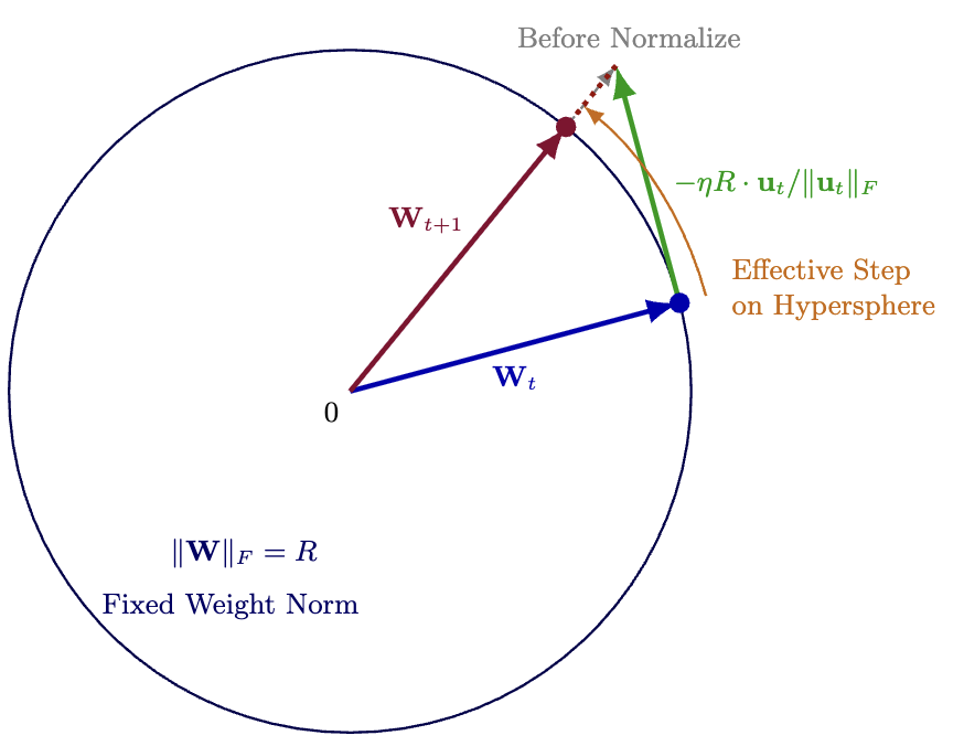
Geometrically, Hyperball constrains the optimization trajectory to the surface of a hypersphere with radius $R$. The update takes a step of length $\eta_t R$ in the direction defined by the normalized update $-\mathrm{Normalize}!\left(u_t\right)$, and the result is immediately projected back onto the sphere. This keeps the norm of the weights and updates constant, so the optimizer navigates primarily through weight directions.

The base update $u_t$ can come from any optimizer. In this paper we focus on Adam Hyperball (AdamH) and Muon Hyperball (MuonH). We apply Hyperball to Transformer weight matrices and use Adam for embeddings, normalization gains, and other parameters whose norm carries semantic information. On $1.2$ B parameter Qwen3 style models ([7]), MuonH achieves $20$ – $30%$ token equivalent speedup over its weight decay counterpart, whereas MuonW gives only about $10%$ at this scale. Across depth and width sweeps, Hyperball keeps the best learning rate window better than the baseline: the maximal drift is about $1.4\times$ for AdamH and MuonH, compared with $2$ – $4\times$ for AdamW and MuonW baselines.

The optimization theory in Section 4.2 explains why this explicit constraint matches the role that weight decay already plays in scale invariant layers. Let $R_t=\left\lVert W_t \right\rVert_\mathrm{F}$ be the Frobenius norm of the parameter matrix, and let $\widehat{W}_t=W_t/R_t$ be its direction. The decomposition $W_t=R_t\widehat{W}_t$ separates radial norm dynamics from directional dynamics: to first order, the angular movement per step scales with the update norm divided by $R_t$. Prior analyses of normalized networks and rotational equilibrium ([8, 9, 10]) show that, under a noise dominated model, decoupled weight decay balances stochastic norm growth and converges to an equilibrium radius. Substituting this radius into the tangent dynamics yields an angular step size $\eta^{\mathrm{ang}}$ that depends on the learning rate and weight decay mainly through the product $\eta \lambda$. Hyperball uses this mechanism directly by fixing the radius and update norm, replacing the indirect calibration of $\lambda$ with an explicit angular learning rate schedule.

2. Method

Section Summary: The Hyperball method keeps selected weight matrices on a sphere of fixed radius R by first taking a step from any base optimizer such as Adam, then immediately rescaling the matrix back to the original norm through simple division by its Frobenius norm. The radius is set once at initialization and the procedure is applied only to attention and MLP weights, while embeddings and other parameters continue to use an ordinary optimizer. The authors prefer this Frobenius-norm version over a spectral-norm alternative because the projection is far cheaper to compute and the matrices observed in practice have high stable rank, making the two constraints behave similarly.

Definition.

Let $W_t$ be the parameter matrix at step $t$, $u_t$ be the base optimizer update for this matrix (for example, Adam's preconditioned update ([11]) or Muon's matrix sign momentum update ([1, 2])), $\eta_t$ be the Hyperball learning rate, $R>0$ be the fixed radius, and $\mathrm{Normalize}!\left(X\right) := X/\left\lVert X \right\rVert_\mathrm{F}$ be Frobenius normalization. For each constrained matrix $W_0 \in \mathbb{R}^{d_{\mathrm{out}}\times d_{\mathrm{in}}}$, we initialize entries with standard deviation $1/\sqrt{d_{\mathrm{in}}}$ and set the radius once as $R=\left\lVert W_0 \right\rVert_\mathrm{F}$. The Hyperball update is

$ W_{t+1} ;=; R \cdot \mathrm{Normalize}!\left(\Big(W_t - \eta_t, R \cdot \mathrm{Normalize}!\left(u_t\right)\Big)\right).\tag{1} $

Thus Hyperball takes an unconstrained optimizer step with norm $\eta_t R$, followed by radial renormalization to radius $R$ (Algorithm 1, Figure 1). Write $\widehat{u}t := u_t/\left\lVert u_t \right\rVert\mathrm{F}$ and $\widehat{W}t := W_t/\left\lVert W_t \right\rVert\mathrm{F}$. Equivalently, the exact displacement is

$ W_{t+1}-W_t

R\left(\frac{\widehat{W}_t-\eta_t\widehat{u}_t} {\left\lVert \widehat{W}_t-\eta_t\widehat{u}t \right\rVert\mathrm{F}} -\widehat{W}_t \right),\tag{2} $

so radial renormalization returns the trial point to the sphere of radius $R$.

Input: parameter matrix $W_t$, base optimizer $\mathcal{O}$, optimizer state $\mathcal{S}_t$, radius $R$, schedule $\{\eta_t\}$
Compute base optimizer update $u_t, S_{t+1} \leftarrow \mathcal{O}(\nabla_{W_t} L(W_t), \mathcal{S}_t)$
Set normalized update direction $\widehat{u}_t \leftarrow \mathrm{Normalize}\!\left(u_t\right)$
Take unprojected step $\widetilde{W}_{t+1} \leftarrow W_t - \eta_t\,R\,\widehat{u}_t$
Project to radius $R$: $W_{t+1} \leftarrow R \cdot \mathrm{Normalize}\!\left(\widetilde{W}_{t+1}\right)$

Where to apply the constraint.

We apply Hyperball to attention and MLP weight matrices in a prenorm Transformer ([5, 6]). Embeddings, normalization gains, and other scalar parameters are updated with a standard optimizer (Adam in our experiments), since for these parameters the norm can carry semantic information.

Discussion of the design.

A natural alternative to the Frobenius norm constraint is a spectral norm constraint. Let $\left\lVert W \right\rVert_{\mathrm{op}}$ denote the operator norm of a matrix. The spectral condition of [12] identifies relative spectral update size as a central quantity for feature learning, and SSO constrains training to the spectral sphere by steepest descent or projection ([13]). In this view, a spectral Hyperball variant would fix $\left\lVert W_t \right\rVert_{\mathrm{op}}$ and normalize the update in operator norm, directly controlling the sharpest layerwise scaling factor.

We use the Frobenius version in Equation 1 for two reasons: computation cost and the theoretical motivation in Section 4. Projection onto the Frobenius sphere is $O(N^2)$ per matrix, whereas exact spectral projection generally requires an SVD and costs $O(N^3)$. One diagnostic for whether Frobenius control is close to spectral control is the stable rank ratio. For a parameter matrix $W \in \mathbb{R}^{d_{\mathrm{out}}\times d_{\mathrm{in}}}$, define

$ \mathcal{R}(W) ;:=; \frac{\left\lVert W \right\rVert_\mathrm{F}^2}{\left\lVert W \right\rVert_{\mathrm{op}}^2} ;\in; [1, , \min(d_{\mathrm{in}}, d_{\mathrm{out}})].\tag{3} $

Values satisfying $\mathcal{R}(W) = \Omega(\min(d_{\mathrm{in}}, d_{\mathrm{out}}))$ indicate that the singular value spectrum is not dominated by a single direction, in which case Frobenius constraints behave similarly to spectral constraints up to a slowly varying factor. The same high stable rank regime is observed empirically in the Kimi Moonlight analysis ([2], Appendix F). A spectral Hyperball variant is a natural direction when singular value concentration makes Frobenius control too loose.

3. Hyperball Experiments

Section Summary: The experiments evaluate Hyperball variants of the Adam and Muon optimizers against their standard weight-decay versions when training language models ranging from 130 million to 8 billion parameters. Across multiple benchmarks, the Hyperball versions deliver larger effective speedups—often 20–30 percent in token-equivalent terms—reach lower validation losses in fewer steps, and match the performance of noticeably larger baseline models. They also keep the best learning rate nearly constant when model depth or width changes by orders of magnitude, unlike the baselines whose optimal rates drift by factors of three or four.

3.1 Setup

Unless noted otherwise, we use a Qwen3 style decoder only architecture ([7]) with QK-Norm ([14]), trained on a mixture of DCLM-baseline ([15]), StarCoder ([16]), and ProofPile 2 ([17]) (and FineWeb-Edu ([18]) for some runs). We compare Adam ([11]) and Muon ([1, 2]) with decoupled weight decay (AdamW and MuonW) against their Hyperball variants AdamH and MuonH. For the speedup metric, we fit a scaling law to AdamW across Chinchilla ratios ([19]) ${1\times, 2\times, 4\times, 8\times}$ and report, for each method's final loss, the token ratio $\tau = N_{\mathrm{AdamW}}/N_{\mathrm{method}}$ that AdamW would need to match it. For learning rate transfer, we sweep a multiplicative grid (ratio $\sqrt{2}$) at each scale $s$, define $\eta^\star(s) := \arg\min_{\eta_k}\ \mathrm{ValLoss}(s, \eta_k; T)$, and report $\mathrm{Drift} := \max_s \eta^\star(s) , /, \min_s \eta^\star(s)$.

3.2 End-to-end speedup

In the weight decay baseline setting adopted from [4], $1.2$ B parameter Qwen3 style models are trained over Chinchilla ratios $1\times$ – $8\times$, and MuonW alone yields $\approx 10%$ token equivalent speedup over the AdamW scaling law. MuonH instead sustains $20$ – $30%$ speedup, and the gap grows with training duration (Figure 2). Qualitatively, Hyperball starts slightly worse but overtakes WD as the learning rate decays. On the Marin speedrun benchmark (FineWeb-Edu, $1\times$ Chinchilla), AdamH and MuonH match WD baselines that are $\approx 10%$ larger (Figure 3, left). In Marin Ferries, scaling MuonH to $8$ B parameters yields a further $0.04$ loss improvement over the AdamW baseline, with both runs using manually chosen hyperparameters (Figure 3, middle and right).

On the public modded-nanogpt Track 3 optimization benchmark, which fixes the model and data and measures optimizer progress by step count, the corresponding WD baselines reach average validation loss $3.2790$ in $5625$ steps for the single run AdamW baseline, $3.2790$ in $3325$ steps for MuonW (tuned), and $3.2789$ in $3250$ steps for NorMuonW ([22]). AdamH reaches average validation loss $3.2741$ in $4875$ steps. MuonH reaches average validation loss $3.2782$ in $3325$ steps, NorMuonH reaches average validation loss $3.2778$ in $3250$ steps, and KL-SOAP-H ([21]) reaches average validation loss $3.2780$ in $3125$ steps (Figure 4) ([23]). This result shows that Hyperball is not tied to Muon or Adam: paired with KL-SOAP, it reaches the fastest loss at step result in this comparison.

3.3 Hyperparameter transfer

By construction, Hyperball fixes $\left\lVert W_t \right\rVert_\mathrm{F}=R$ and uses unit Frobenius update directions, so $\eta_t$ directly sets the relative update length. The optimal learning rate should therefore be approximately scale invariant. We test this in two sweeps with $10$ B tokens per run. These transfer runs use a hybrid normalization architecture variant ([24]), with QK-Norm enabled.

For depth scaling at fixed hidden dimension $d=128$ and $L \in {4, \dots, 512}$, the maximal drift of the optimal learning rate is $\approx 1.4\times$ for AdamH and MuonH, versus $\approx 3\times$ for AdamW and $\approx 4\times$ for MuonW even at $L=512$ (Figure 5).

For width scaling at fixed depth $L=4$ and $d \in {128, \dots, 2048}$, the same $\approx 1.4\times$ drift holds for both Hyperball variants (Figure 6).

3.4 Overtrained Setting

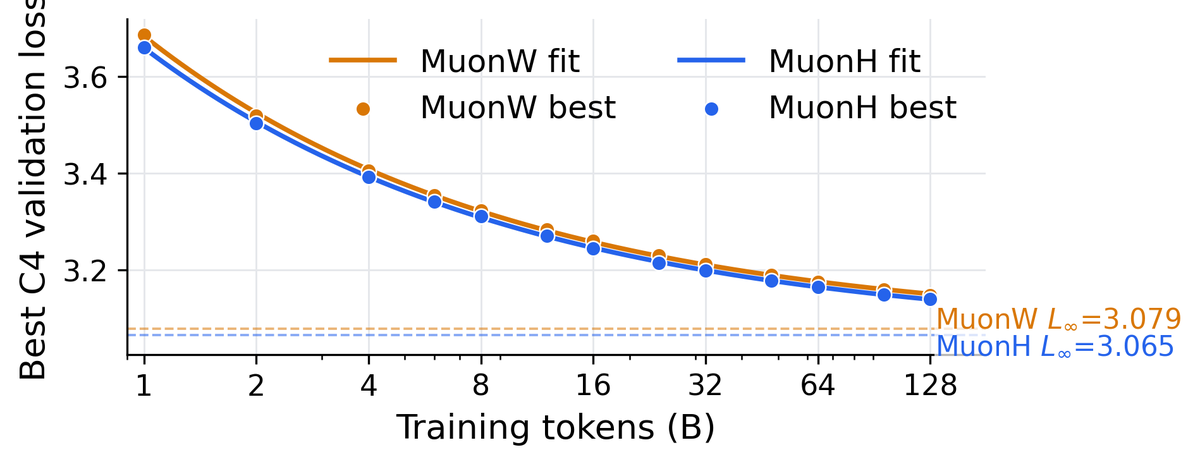
We also test Hyperball in an overtrained data scaling setting. For a $130$ M parameter model, we train MuonW and MuonH over token budgets from $1$ B to $128$ B and sweep the learning rate at each budget. Both MuonW and MuonH use the same hybrid normalization architecture variant as in previous section. MuonH attains lower best C4 validation loss across the full range (Figure 7). Fitting $L(N)=L_\infty + A N^{-\alpha}$ to the best loss curve gives $L_\infty=3.065$ for MuonH versus $3.079$ for MuonW.

4. Theory

Section Summary: The theory section explains that normalization layers with trainable gains preserve a network’s full expressive power even when weight-matrix norms are constrained, since any rescaling of the weights can be exactly offset by the gain parameters. It then analyzes optimization under scale-invariant losses, which depend only on the direction of each weight matrix rather than its magnitude; in this setting, decoupled weight decay indirectly controls the size of angular steps on the unit sphere and therefore the speed of progress in function space. The discussion illustrates these dynamics with idealized AdamW and Muon updates under simplifying assumptions of infinite training history and isotropic gradients.

4.1 Expressivity

We first show that, in normalized networks, fixing the Frobenius norm of a weight matrix wouldn't limit representation power. This is because a trainable normalization gain can absorb the scale of the weight matrix, so Hyperball changes the optimization geometry without removing represented functions. Let $h$ be the hidden state, $W$ be a weight matrix, and $\gamma$ be the RMSNorm gain ([25]). For a a linear map placed after a layer norm,

$ f(h;W, \gamma) ;=; W, (\gamma \odot \mathrm{RMSNorm}(h)).\tag{4} $

For any scalar $c>0$, the joint rescaling $(W, \gamma) \mapsto (cW, \gamma/c)$ leaves the represented function unchanged:

$ f(h;cW, \gamma/c) = f(h;W, \gamma).\tag{5} $

Thus constraining $\left\lVert W \right\rVert_\mathrm{F}$ need not reduce the represented function class when a trainable normalization gain can absorb the scale.

4.2 Optimization

With $W$ being a parameter block and $\mathcal{W}^c$ being the remaining parameters in the neural network. A loss $L(W, \mathcal{W}^c)$ is scale invariant in a parameter block $W$ if $L(cW, \mathcal{W}^c) = L(W, \mathcal{W}^c)$ for all $c>0$. We will drop $\mathcal{W}^c$ and use the shorthand $L(W)$ from now on. This is the notion used throughout the analysis: the radial coordinate $\left\lVert W \right\rVert_\mathrm{F}$ is redundant, and the loss depends only on the direction $\widehat{W} = W/\left\lVert W \right\rVert_\mathrm{F}$. Many weight matrices in modern LLMs are only approximately scale invariant in this loss level sense, but the exact scale invariant model is a useful local approximation for the norm dynamics below.

Decoupled weight decay and angular motion.

Let $W_t$ be the parameter matrix at step $t$, $u_t$ be the base optimizer update for this matrix, $\eta_t$ be the learning rate, $\lambda$ be the weight decay coefficient, and $\alpha_t := 1-\eta_t \lambda$. The standard decoupled weight decay update ([3]) is

$ W_{t+1} = \alpha_t W_t - \eta_t u_t.\tag{6} $

Let $R_t := \left\lVert W_t \right\rVert_\mathrm{F}$ and $\widehat{W}_t := W_t/R_t$. The angular step size is the per step movement on the unit sphere,

$ \eta^{\mathrm{ang}}t := \left\lVert \widehat{W}{t+1}-\widehat{W}t \right\rVert\mathrm{F},\tag{7} $

and the relative update ratio is

$ \rho_t := \left\lVert u_t \right\rVert_\mathrm{F}/\left\lVert W_t \right\rVert_\mathrm{F}.\tag{8} $

For scale invariant $L$, the function represented by the block is determined by $\widehat{W}_t$, so $\eta^{\mathrm{ang}}_t$ is the optimizer-controlled quantity that determines how fast this block moves in function space. The direction after one decoupled step is exactly

$ \widehat{W}_{t+1}

\frac{\alpha_t\widehat{W}_t - \eta_t u_t/R_t} {\left\lVert \alpha_t\widehat{W}t - \eta_t u_t/R_t \right\rVert\mathrm{F}}.\tag{9} $

Thus, for fixed $\left\lVert u_t \right\rVert_\mathrm{F}$, a larger radius $R_t$ gives a smaller angular movement. Weight decay therefore acts as an indirect angular step controller by regulating $R_t$.

Concrete base updates.

The analysis below uses AdamW, Muon, and Moonlight scaled Muon as examples. Let $\ell_t$ be the minibatch loss, $g_t := \nabla_W\ell_t(W_t)$ be the stochastic gradient for the matrix block, let $\epsilon>0$ be Adam's numerical stability constant, and let divisions and square roots in Adam be elementwise. For AdamW ([3]),

$ m_t = \beta_1 m_{t-1} + (1-\beta_1)g_t, \qquad v_t = \beta_2 v_{t-1} + (1-\beta_2)g_t^{\odot 2}, \qquad u_t = \frac{\widehat{m}_t}{\sqrt{\widehat{v}_t}+\epsilon},\tag{10} $

where $\widehat{m}_t$ and $\widehat{v}_t$ denote the bias corrected moments. For Muon ([1, 2]), let

$ M_t = \beta_1M_{t-1} + (1-\beta_1)g_t.\tag{11} $

For a matrix $A$ with compact singular value decomposition $A=P\Sigma Q^\top$, define the exact SVD matrix sign map by

$ \operatorname{msign}(A) := P Q^\top.\tag{12} $

Muon implementations often compute this map by Newton–Schulz iteration; in this theory we analyze the idealized SVD Muon update. For $W\in \mathbb{R}^{d_{\mathrm{out}}\times d_{\mathrm{in}}}$, define $s_\mu:=\max(1, \sqrt{d_{\mathrm{out}}/d_{\mathrm{in}}})$. The Muon base update is

$ u_t = s_\mu, \operatorname{msign}(M_t).\tag{13} $

Moonlight ([2]) uses the same momentum and exact SVD sign map, but replaces $s_\mu$ with $s_{\mathrm{moon}}:=0.2\sqrt{\max(d_{\mathrm{in}}, d_{\mathrm{out}})}$:

$ u_t = s_{\mathrm{moon}}, \operatorname{msign}(M_t).\tag{14} $

Idealized stationary model.

We first make an assumption that assume we have an infinite history of gradient. This allows us to ignore boundary conditions on gradient when we consider momentum and weights.

########## {caption="Assumption 1: Infinite history optimizer"}

The gradient sequence ${g_t}{t\in\mathbb Z}$ and the weight sequence ${W_t}{t\in\mathbb Z}$ are defined for all integer times, including $t<0$. Optimizer states are computed from this infinite past, i.e.,

$ m_t=(1-\beta_1)\sum_{i\ge0}\beta_1^i g_{t-i}, \qquad M_t=(1-\beta_1)\sum_{i\ge0}\beta_1^i g_{t-i}.\tag{15} $

In the constant learning rate calculation below, $W_t$ is also taken to be the solution obtained by running Equation 6 from the infinite past. Intuitively, this describes the regime where training has already run for a long time, so the dependence on the initial optimizer state and initial weight has decayed.

We then make the following assumption on the distribution of $g_t$.

########## {caption="Assumption 2: Isotropic stationary gradients and idealized base maps"}

Let $p=d_{\mathrm{out}}$, $q=d_{\mathrm{in}}$, $d=pq$, and $r=\min(p, q)$. After vectorizing the matrix block, the stochastic optimizer input is an iid isotropic Gaussian sequence,

$ g_t\sim\mathcal N(0, \sigma^2 I_d), \qquad {g_t}_{t\in\mathbb Z}\text{ independent.}\tag{16} $

Section 4.2 is intentionally idealized. It ignores anisotropy, layer specific structure, and the signal in $\mathbb{E}[g_t]$. Its purpose is to provide an easy to compute ansatz for update norms, update autocorrelations, radial equilibria, and angular step sizes.

For AdamW, we consider an idealized AdamW update by assuming that the second moment is correctly estimated. For a scalar coordinate $\bar{g}_t$ with $\mathbb{E}[\bar{g}_t^2]=\sigma^2$, the stationary Adam second moment satisfies

$ \mathbb{E}[v_t]

(1-\beta_2)\sum_{i\ge0}\beta_2^i, \mathbb{E}[\bar{g}_{t-i}^2]

(1-\beta_2)\sum_{i\ge0}\beta_2^i, \sigma^2

\sigma^2.\tag{17} $

We therefore replace the Adam denominator by $\sigma$ and ignore the vanishing bias correction transient:

$ u_t = \frac{m_t}{\sigma}, \qquad m_t=(1-\beta_1)\sum_{i\ge 0}\beta_1^i g_{t-i}.\tag{18} $

Update norm and autocorrelation.

We will first study the correlation between updates at different steps, referred to as update autocorrelation.For Muon, the update autocorrelation is related to the following matrix sign map.

For $\rho\in[-1, 1]$, define the SVD Muon sign kernel

$ \kappa_{p, q}(\rho) := \frac{1}{\min(p, q)}, \mathbb{E}\Big[\left\langle \operatorname{msign}(X), , \operatorname{msign}(\rho X + \sqrt{1-\rho^2}, Z) \right\rangle\Big],\tag{19} $

where $X, Z\in \mathbb{R}^{p\times q}$ have iid $\mathcal N(0, 1)$ entries and are independent. The normalization gives $\kappa_{p, q}(1)=1$ and $\kappa_{p, q}(0)=0$.

########## {caption="Lemma 3: Update norm and update autocorrelation"}

Under Section 4.2 and Section 4.2, define the update scale $U$ by

$ U = \begin{cases} \sqrt{\dfrac{1-\beta_1}{1+\beta_1}}, \sqrt{pq} & \text{(idealized AdamW)}, \ \sqrt{p} & \text{(SVD Muon)}, \ 0.2\sqrt{pq} & \text{(Moonlight scaled SVD Muon)}, \end{cases}\tag{20} $

Define the normalized autocorrelation sequence by $c_0=1$ and, for every lag $h\ge 1$,

$ c_h= \begin{cases} \beta_1^h & \text{(idealized AdamW)}, \ \kappa_{p, q}(\beta_1^h) & \text{(SVD Muon and Moonlight scaled SVD Muon)}. \end{cases}\tag{21} $

For every lag $h\ge1$, these definitions give the second moment identities

$ \mathbb{E}\left\lVert u_t \right\rVert_\mathrm{F}^2=U^2, \qquad \mathbb{E}\left\langle u_t, , u_{t-h} \right\rangle=U^2c_h.\tag{22} $

Proof: For AdamW, each coordinate of Equation 18 is a stationary Gaussian moving average. If $\bar{g}_t$ is one coordinate, then

$ \bar{u}t=(1-\beta_1)\sum{i\ge0}\beta_1^i\frac{\bar{g}_{t-i}}{\sigma}.\tag{23} $

Thus $\mathbb{E}[\bar{u}_t^2]=(1-\beta_1)/(1+\beta_1)$. For lag $h\ge1$,

$ \mathbb{E}[\bar{u}t\bar{u}{t-h}]

\frac{1-\beta_1}{1+\beta_1}, \beta_1^h.\tag{24} $

Summing over $d=pq$ independent coordinates gives the AdamW line of Equation 20 and both identities in Equation 22, with $c_h=\beta_1^h$.

For SVD Muon, $\operatorname{msign}(A)$ has exactly $r=\min(p, q)$ nonzero singular values, all equal to $1$. Therefore

$ \left\lVert s_\mu \operatorname{msign}(M_t) \right\rVert_\mathrm{F}^2 =s_\mu^2 r =\max(1, p/q)\min(p, q) =p,\tag{25} $

which gives $U=\sqrt p$. For Moonlight, the same calculation gives

$ \left\lVert s_{\mathrm{moon}}\operatorname{msign}(M_t) \right\rVert_\mathrm{F}^2 =0.04\max(p, q)\min(p, q) =0.04pq,\tag{26} $

so $U=0.2\sqrt{pq}$.

It remains to identify the autocorrelation. The stationary momentum matrices satisfy

$ M_t=(1-\beta_1)\sum_{i\ge0}\beta_1^i g_{t-i}.\tag{27} $

Hence each pair $(M_t, M_{t-h})$ is jointly Gaussian, with identical marginal covariance and entrywise correlation $\beta_1^h$ using standard property of geometric sequences. After dividing both matrices by their common standard deviation, the pair has the same distribution as

$ \bigl(X, , \beta_1^h X + \sqrt{1-\beta_1^{2h}}, Z\bigr),\tag{28} $

with $X, Z$ as in Equation 19. Because the matrix sign is invariant to positive scalar rescaling, the normalized expected inner product of the two SVD Muon updates is exactly $\kappa_{p, q}(\beta_1^h)$. Multiplying by $s_\mu^2r=U^2$ or $s_{\mathrm{moon}}^2r=U^2$ gives the autocorrelation identity in Equation 22. The scalar multiplier $s_\mu$ or $s_{\mathrm{moon}}$ cancels in the normalized autocorrelation, so Muon and Moonlight share the same $c_h$.

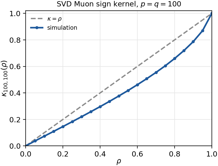
One question is what the range is for $\kappa_{p, q}$. Let $F(X):=r^{-1/2}\operatorname{msign}(X)$. Since $F(-X)=-F(X)$ and $X$ is symmetric, $\mathbb{E}[F(X)]=0$ and $\mathbb{E}\left\lVert F(X) \right\rVert_\mathrm{F}^2=1$. By the Hermite expansion of the Gaussian noise operator,

$ \kappa_{p, q}(\rho)=\sum_{k\ge1} a_k\rho^k, \qquad a_k\ge0, \qquad \sum_{k\ge1}a_k=1.\tag{29} $

Therefore, for $0\le\rho\le1$,

$ 0\le\kappa_{p, q}(\rho)\le\rho.\tag{30} $

This inequality will be used later to show the correlation between weight and update is bounded. Figure 8 illustrates this range in a numerical simulation with $p=q=100$.

Weight update correlation.

We will now consider constant hyperparameter training, the case where we use constant learning rate $\eta$ and constant weight decay $\lambda$. We denote $1-\eta \lambda$ as $\alpha$, and assume $0<\alpha<1$.

########## {caption="Lemma 4: Stationary projection coefficient"}

Under Section 4.2 and Section 4.2 and constant hyperparameter training, let the normalized update autocorrelation sequence $c_h$ be given by Equation 21. Let

$ C_\alpha := \sum_{h=1}^{\infty}\alpha^{h-1}c_h.\tag{31} $

Define $\gamma_t:= \mathbb{E}\left\langle W_t, , u_t \right\rangle/U^2$ to be the projection coefficient, quantifying how strongly the weight and update correlates, then $\gamma_t$ identically equal to a constant value $\gamma$ for all $t$, with

$ \gamma=-\eta C_\alpha.\tag{32} $

Proof: Since $0<\alpha<1$, the stationary solution of the decoupled weight decay recursion Equation 6 is

$ W_t=-\eta\sum_{h=1}^{\infty}\alpha^{h-1}u_{t-h}.\tag{33} $

Taking the expectation of the inner product with $u_t$ and using Equation 22 gives

$ \mathbb{E}\left\langle W_t, , u_t \right\rangle

-\eta\sum_{h=1}^{\infty}\alpha^{h-1}\mathbb{E}\left\langle u_{t-h}, , u_t \right\rangle

-\eta U^2\sum_{h=1}^{\infty}\alpha^{h-1}c_h.\tag{34} $

Dividing by $U^2$ and using the definition of $C_\alpha$ in Equation 31 proves Equation 32.

For AdamW, $c_h=\beta_1^h$, and the sum can be simplified,

$ \begin{aligned}C_\alpha^{\mathrm{Adam}} &= \sum_{h=1}^{\infty}\alpha^{h-1}\beta_1^h\&= \beta_1\sum_{h=1}^{\infty}(\alpha\beta_1)^{h-1} = \frac{\beta_1}{1-\alpha\beta_1}.\end{aligned}\tag{35} $

For SVD Muon and Moonlight,

$ C_\alpha^{\mathrm{Muon}}=C_\alpha^{\mathrm{Moonlight}} =\sum_{h=1}^{\infty}\alpha^{h-1}\kappa_{p, q}(\beta_1^h).\tag{36} $

The series is finite because Equation 30 gives $c_h\le\beta_1^h$. The negative sign means that, in stationarity, the current update is negatively correlated with the current weight. The size of this negative correlation is controlled by $C_\alpha$. Substituting Equation 35 into Equation 32 recovers the familiar AdamW expression

$ \gamma

-\eta C_\alpha^{\mathrm{Adam}}

-\eta\frac{\beta_1}{1-\alpha\beta_1}

-\frac{\eta\beta_1}{1-\alpha\beta_1}.\tag{37} $

Equilibrium weight norm.

Let stationary weight norm $S_t:= \mathbb{E}\left\lVert W_t \right\rVert_\mathrm{F}^2$ and let $U^2$ be the update second moment in Equation 22. Squaring Equation 6, taking expectations, and substituting $\mathbb{E}\left\langle W_t, , u_t \right\rangle=\gamma U^2$ gives the following equality:

$ S_{t+1}

\alpha^2 S_t+\eta^2U^2-2\alpha \eta\gamma U^2.\tag{38} $

At stationarity, $S_{t+1}=S_t=R_\star^2$, and 32 gives

$ R_\star

\eta U\sqrt{\frac{1+2\alpha C_\alpha}{1-\alpha^2}}.\tag{39} $

For AdamW, Equation 35 reduces this to the previous closed form

$ R_\star^{\mathrm{Adam}}

\eta U\sqrt{\frac{1+\alpha\beta_1}{(1-\alpha^2)(1-\alpha\beta_1)}}.\tag{40} $

For SVD Muon and Moonlight, the correct formula is instead Equation 39 with $C_\alpha$ from Equation 36. In all cases, when $\eta \lambda$ is small and $\beta_1$ is fixed, $R_\star=\Theta(U\sqrt{\eta/\lambda})$ up to the autocorrelation factor $\sqrt{1+2\alpha C_\alpha}$. Closely related estimates for AdamW update and weight RMS based on mean field approximation appear in [26, 27, 28].

########## {caption="Corollary 5: Cosine and angular step at equilibrium"}

Under Section 4.2 and Section 4.2 and constant hyperparameter training, the following cosine proxy between the weight and update $\cos_t:=\frac{\mathbb{E}\left\langle W_t, , u_t \right\rangle}{R_\star U}$ identically equal to a constant value $\cos_\star$ for all $t$, with

$ \cos_\star = -C_\alpha\sqrt{\frac{1-\alpha^2}{1+2\alpha C_\alpha}}.\tag{41} $

The corresponding ansatz angular step size at equilibrium is

$ (\eta^{\mathrm{ang}})^2

\frac{2(1-\alpha)\bigl(1-(1-\alpha)C_\alpha\bigr)}{1+2\alpha C_\alpha}.\tag{42} $

For AdamW, this becomes

$ {\eta^{\mathrm{ang}}}

\sqrt{\frac{2(1-\alpha)(1-\beta_1)}{1+\alpha\beta_1}}

\sqrt{\frac{2 \eta \lambda(1-\beta_1)}{1+(1-\eta \lambda)\beta_1}}.\tag{43} $

Proof: The cosine formula follows from $\mathbb{E}\left\langle W_t, , u_t \right\rangle=\gamma U^2$, $\gamma=-\eta C_\alpha$, and 39:

$ \cos_\star=\frac{\gamma U}{R_\star} =-C_\alpha\sqrt{\frac{1-\alpha^2}{1+2\alpha C_\alpha}}.\tag{44} $

For the angular step, plug $\mathbb{E}\left\langle W_t, , u_t \right\rangle=\gamma U^2$ and $R_t=R_\star$ into Equation 9, and set $k_\star:=U/R_\star$. This gives

$ \left\langle \widehat{W}_{t+1}, , \widehat{W}_t \right\rangle

\frac{\alpha-\eta\gamma k_\star^2} {\sqrt{\alpha^2-2\alpha \eta\gamma k_\star^2+\eta^2k_\star^2}}.\tag{45} $

At equilibrium, the denominator equals $1$ by the stationary radius equation. Using $k_\star^2=(1-\alpha^2)/(\eta^2(1+2\alpha C_\alpha))$ and $\gamma=-\eta C_\alpha$ gives

$ (\eta^{\mathrm{ang}})^2 =2-2\left(\alpha+\frac{C_\alpha(1-\alpha^2)}{1+2\alpha C_\alpha}\right) =\frac{2(1-\alpha)\bigl(1-(1-\alpha)C_\alpha\bigr)}{1+2\alpha C_\alpha}.\tag{46} $

Substituting $C_\alpha=\beta_1/(1-\alpha\beta_1)$ gives Equation 43.

########## {caption="Theorem 6: Weight decay sets equilibrium radius and angular step size"}

Under Section 4.2 and Section 4.2 and constant hyperparameter training with $\alpha=1-\eta \lambda$, the weight in the decoupled weight decay update Equation 6 will converge to the equilibrium radius Equation 39. At this equilibrium, the angular step size is given by Equation 42, with the AdamW specialization Equation 43. The base optimizer enters through two quantities only: the update norm $U$ and the autocorrelation sum $C_\alpha$.

Proof: By Lemma 4, $\mathbb{E}\left\langle W_t, , u_t \right\rangle=\gamma U^2$ with $\gamma=-\eta C_\alpha$. The radial recursion Equation 38 then gives Equation 39, and Corollary 5 gives the angular step size.

Under Section 4.2 and Section 4.2, the optimizer enters through the identities in Equation 22. Once $U$ and $c_h$ are fixed, the weight decay recursion determines the stationary radius, cosine proxy, and angular step algebraically.

Table 1 consolidates the stationary quantities. The update norm $U$ controls the equilibrium radius. The autocorrelation sum $C_\alpha$ controls the momentum-induced radial correction, the cosine, and the angular step. AdamW has $C_\alpha=\beta_1/(1-\alpha\beta_1)$, whereas SVD Muon and Moonlight use the matrix sign kernel in Equation 36.

\begin{tabular}{@{\hspace{5pt}}l@{\hspace{8pt}}|@{\hspace{8pt}}ccc@{\hspace{5pt}}}
\toprule
Quantity & AdamW & SVD Muon & Moonlight SVD Muon \\
\midrule
Update norm $U$
   {} & $\sqrt{\tfrac{1-\beta_1}{1+\beta_1}}\, \sqrt{d_{\mathrm{in}}d_{\mathrm{out}}}$
   {} & $\sqrt{d_{\mathrm{out}}}$
   {} & $0.2\sqrt{d_{\mathrm{in}}d_{\mathrm{out}}}$ \\
Autocorr. sum $C_\alpha$
   {} & $\dfrac{\beta_1}{1-\alpha\beta_1}$
   {} & $\sum_{h\ge1}\alpha^{h-1}\kappa_{p, q}(\beta_1^h)$
   {} & $\sum_{h\ge1}\alpha^{h-1}\kappa_{p, q}(\beta_1^h)$ \\
Equilibrium norm $R_\star$
   {} & \multicolumn{3}{c}{$\eta U\sqrt{\dfrac{1+2\alpha C_\alpha}{1-\alpha^2}}$} \\
Cosine proxy $\cos_\star$
   {} & \multicolumn{3}{c}{$-C_\alpha\sqrt{\dfrac{1-\alpha^2}{1+2\alpha C_\alpha}}$} \\
Angular step size $(\eta^{\mathrm{ang}})^2$
   {} & \multicolumn{3}{c}{$\dfrac{2(1-\alpha)\bigl(1-(1-\alpha)C_\alpha\bigr)}{1+2\alpha C_\alpha}$} \\
\bottomrule
\end{tabular}

########## {caption="Lemma 7: Inverse gradient scaling for scale invariant losses"}

Independently of Section 4.2 and Section 4.2, if $L: \mathbb{R}^{d_{\mathrm{out}}\times d_{\mathrm{in}}}\to \mathbb{R}$ is differentiable and scale invariant, $L(cW)=L(W)$ for all $c>0$, then

$ \nabla_W L(cW)=\frac{1}{c}\nabla_W L(W) \qquad\text{for all }c>0.\tag{47} $

Proof: Scale invariance gives $L(cW+c\epsilon)=L(W+\epsilon)$ for every matrix $\epsilon$. Differentiating both sides with respect to $\epsilon$ at $\epsilon=0$ gives

$ \left\langle \nabla_W L(cW), , c\epsilon \right\rangle=\left\langle \nabla_W L(W), , \epsilon \right\rangle \qquad\forall\epsilon,\tag{48} $

which forces $c\nabla_W L(cW)=\nabla_W L(W)$.

Applying Lemma 7 to $W_t=R_t\widehat{W}_t$ gives

$ \left\lVert \nabla_W L(W_t) \right\rVert_\mathrm{F}

\frac{1}{R_t}\left\lVert \nabla_W L(\widehat{W}t) \right\rVert\mathrm{F}.\tag{49} $

Combined with $R_\star\propto\sqrt{\eta/\lambda}$ from Equation 39, this gives the scale invariant prediction $\left\lVert \nabla_W L(W_t) \right\rVert_\mathrm{F}\propto\sqrt{\lambda/\eta_t}$ when the direction of the weight is fixed and the autocorrelation factor changes slowly.

Interpretation.

The main message of the theory is that, for scale invariant matrix blocks, decoupled weight decay should be understood as an indirect controller of angular optimization speed rather than merely as a regularizer. The preceding results make this mechanism explicit:

1. For a scale invariant loss, the relevant optimization variable is the direction $\widehat{W}=W/\left\lVert W \right\rVert_\mathrm{F}$, and the effective angular step is controlled by the angular learning rate $\eta^{\mathrm{ang}}t := \left\lVert \widehat{W}{t+1}-\widehat{W}t \right\rVert\mathrm{F}$.
2. Lemma 3 shows that for common optimizer the update norm $U$ and the correlation for update between steps converge to constants that only depend on optimizer choices and hyperparameters.
3. Lemma 4 and Theorem 6 show that (1) weight converges to an equilibrium radius $R_\star$ and (2) the angular learning rate converge to a constant $\eta^{\mathrm{ang}}$ and both constant only depend on optimizer choices and hyperparameters.
4. Lemma 7 shows that, for scale invariant losses, larger equilibrium radius imply smaller gradient norms, giving the prediction $\left\lVert \nabla_W L(W_t) \right\rVert_\mathrm{F}\propto 1/R_t$ when the direction remains unchange.

Thus, weight decay has two coupled effects: it fixes the radial scale $R_\star$, and that radial scale determines the angular learning speed through $\left\lVert u_t \right\rVert_\mathrm{F}/R_\star$. This is the mechanism that Hyperball makes explicit: instead of letting weight decay indirectly determine both the matrix norm and the relative update length, Hyperball fixes the norm and the normalized update length directly.

4.3 Empirical Validation

Phenomenon 1: weight norm tracks learning rate warmup and decay throughout training.

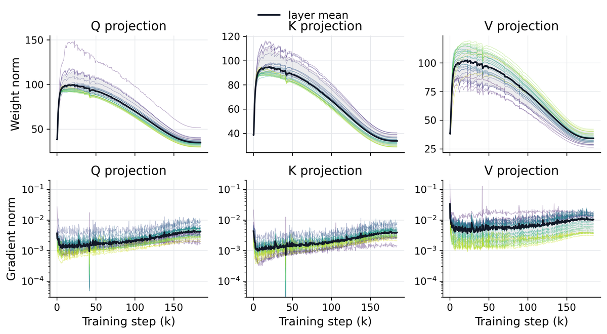
Under a WSD learning rate schedule, Equation 39 predicts that $R_t$ should rise during warmup and shrink during learning rate decay. In a $1.2$ B AdamW run with cosine learning rate decay, Q/K/V projection norms across layers show exactly this pattern: norms rise rapidly during warmup and then decrease during decay (Figure 9, top).

Phenomenon 2: gradient norm increases through training.

For scale invariant blocks, Equation 49 predicts that gradient norms scale approximately as $1/R_t$. This phenomenon is also studied in [29], where a similar explanation is provided. In the same run, the corresponding Q/K/V gradient norms increase late in training as the weight norms shrink during learning rate decay (Figure 9, bottom).

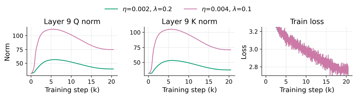
Phenomenon 3: when $\eta \lambda$ is fixed, AdamW converges to essentially the same loss while each matrix norm is roughly proportional to $\eta$.

Theorem 6 predicts that holding $\eta \lambda$ fixed keeps the angular step size $\eta^{\mathrm{ang}}$ nearly fixed, so the training loss should be nearly unchanged. Furthermore, if we divide $\lambda$ by $c$ and multiply $\eta$ by $c$, then Equation 39 predicts $R_\star \propto c$. In Figure 10, we present two runs with $(\eta, \lambda)=(0.002, 0.2)$ and $(0.004, 0.1)$, and we observe that the train loss curves nearly overlap, while the equilibrium Q/K norms are roughly doubled in the larger learning rate run.

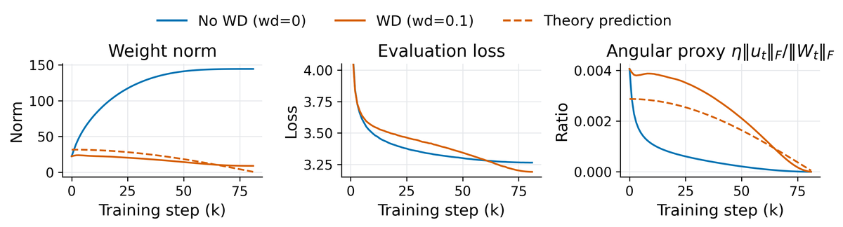
Phenomenon 4: despite sharing the same learning rate schedule, weight decay starts with a higher loss but ultimately converges lower than no weight decay.

When the WD and no WD runs use the same learning rate warmup and decay schedule, Equation 39 and 43 predict different weight norms and angular step dynamics. Without WD, the weight norm grows and the angular proxy $\eta\left\lVert u_t \right\rVert_\mathrm{F}/\left\lVert W_t \right\rVert_\mathrm{F}$ decays. With WD, the run maintains a larger effective step size throughout training. Empirically, and in the theory in Section 4.2, training with WD yields a larger effective step size than training without WD. According to the river valley theory ([30]), the loss decomposes into a "river" component, capturing progress along a relatively flat direction where long term optimization happens, and a "hill" component, capturing excursions in steep directions caused by stochastic gradients. A larger effective step size amplifies these hill direction oscillations, which raises the observed loss early in training, but it also accelerates motion along the river. When the learning rate decays, the oscillations in the hill directions shrink and the iterate settles closer to the riverbed, revealing the additional progress that has already been made along the river. This theory agrees with the phenomenon we observed here. The WD run starts with a higher loss but ultimately reaches a lower loss, because its larger effective step size allows it to move faster down the river before the decay phase suppresses the oscillations (Figure 11).

Phenomenon 5: contrary to the original $\mu$ P prediction, transfer is not sensitive to weight scale at initialization but is sensitive to weight decay scaling.

Recent hyperparameter transfer studies find that transfer is often less sensitive to the initial weight scale than to how weight decay is scaled across model size and training duration ([31, 32, 33, 34, 35]). This is consistent with Equation 39: the radial recursion forgets the initial radius and converges to a norm set by $\eta$, $\lambda$, and the optimizer dependent update norm $U$. Changing the scaling rule for $\lambda$, however, changes both the equilibrium norm $R_\star$ and the angular step size in Equation 43, so it changes the dynamics relevant to transfer that are assumed by $\mu$ P style analyses ([36]). Hyperball turns this dependence into an explicit design choice by fixing the radius and normalized update length directly, which is why the same learning rate window transfers better across depths and widths in Section 3.3.

5. Related work

Section Summary: Earlier research showed that weight decay in networks using normalization layers like BatchNorm often influences training dynamics through effects on weight norms and effective step sizes, rather than simply limiting model capacity. A range of prior methods have decoupled weight magnitudes from directions via reparameterization tricks or specialized optimizers that project or constrain updates, including approaches like Weight Normalization and AdamP. In the context of large language models, recent work has explored enforcing fixed norms during pretraining or optimizing on manifolds, though Hyperball stands out by applying a direct, lower-cost projection to control both weight and update sizes at the full matrix level.

Weight decay in normalized networks.

Earlier work showed that, in normalized networks, weight decay often changes optimization dynamics or effective learning rates rather than acting as a classical capacity penalty ([37, 38, 39, 40]). A line of work argues that, in the presence of BatchNorm ([41]) or LayerNorm ([42]), weight decay acts through norm dynamics: it sets an equilibrium weight norm and, jointly with the learning rate, an angular step size ([8, 9, 10]). [12] formalize the role of the relative update size in feature learning at scale via a spectral condition. Our analysis of Section 4 sits squarely in this picture, closest in spirit to the rotational equilibrium framework of [10]. Hyperball is the matrix level wrapper that pins the relevant ratio directly rather than letting it equilibrate.

Norm constraints on weights and updates.

Decoupling weight magnitude from direction has a long history. Weight Normalization ([43]) reparameterizes $W=g, V/\left\lVert V \right\rVert$. Weight Standardization and BiT ([44, 45]) standardize kernel statistics. Convolutional Normalization ([46]) reduces per layer spectral norm. Decoupled Networks ([47]) split feature norm from angle. Artificial Kuramoto Oscillatory Neurons ([48]) use unit norm oscillator states. On the update side, AdamP and SGDP ([49]) project updates onto the tangent space of the weight direction, Lion ([50]) fixes the per entry update magnitude via the sign function, and LionAR normalizes early update sizes using angular criteria ([51]). For generative models, EDM2 ([52]) normalizes column weights and Spectral Normalization ([53]) bounds the operator norm. Hyperball differs in being an optimizer wrapper that simultaneously fixes the matrix Frobenius norm and the update Frobenius norm, exposing the directional step size as a designed quantity.

Fixed norms in LLM pretraining and manifold optimization.

Several recent and concurrent works enforce normalization at the architecture or optimizer level for language model pretraining. nGPT ([54]) enforces columnwise unit norms with adaptive normalization layers. Nemotron-Flash ([55]) applies per channel spherical constraints for inference time benefits but not on updates. The approximately normalized Transformer (anGPT) ([56]) bounds each weight row using constrained parameter regularization ([57]). [58] periodically rescale weights toward a target variance. On richer manifolds, Modular Manifolds ([59]), Muon $+$ Stiefel ([60]), notes on orthogonal manifolds and steepest descent ([61, 62]), and [63] optimize on the Stiefel or spectral sphere manifold. Related spectral norm views of Muon and weight decay appear in [64, 65], while SSO ([13]) performs steepest descent or projection to the spectral sphere. Hyperball projects onto the matrix Frobenius sphere $S^{d_{\mathrm{in}}d_{\mathrm{out}}-1}$ —a softer constraint than normalization by column or channel—at $O(N^2)$ cost per matrix, versus $O(N^3)$ for spectral projections.

6. Conclusion

Section Summary: Hyperball introduces an explicit constraint on matrix and update norms in the optimizer, replacing the indirect control typically provided by weight decay. Experiments show this approach leads to more consistent performance as models grow in size or depth and makes it easier to transfer learning rates across different training setups. Future work could explore alternative norm constraints and develop a clearer theory of how fixing these norms influences the overall training process.

Hyperball replaces the implicit norm control of weight decay with an explicit optimizer constraint on matrix norms and update norms. Across our experiments, the explicit constraint improves the scaling behavior of matrix based optimizers and makes learning rate transfer more reliable across model widths, depths, and training budgets.

A broader question is which constraint should be imposed. The Frobenius norm is computationally cheap and theoretically motivated by the mechanism studied here, but spectral, rowwise, columnwise, hybrid, or architecture dependent constraints may better match some models and optimizers. Another direction is to develop a sharper theory of weight normalized training, including Weight Normalization style parameterizations ([43]) and explicit norm constraints: when the radial degree of freedom is removed or fixed, how does this shape the training trajectory?

Acknowledgments

Section Summary: The authors received financial support through fellowships and grants from Stanford University and the National Science Foundation, along with computing resources from Google programs, for work connected to the Marin Project. They credit several colleagues with sparking the research idea and express gratitude to a long list of others for helpful conversations. The project serves as an early demonstration that optimizers can be designed to manage weight sizes directly, removing the need for weight decay.

Kaiyue Wen acknowledges support from the Stanford Graduate Fellowship. Tengyu Ma acknowledges support from NSF grant 2522743. This work was supported by the Google TPU Research Cloud (TRC), the Stanford HAI–Google Cloud Credits Program, and NSF RI 2045685, and is part of the Marin Project. The authors would like to thank Songlin Yang, Zihan Qiu, and Liliang Ren for motivating this project. To some extent, this work is a proof of concept showing that it is possible to remove weight decay altogether by designing optimizers that explicitly control weight norms. The authors would also like to thank William Held, David Hall, Suhas Kotha, Tatsunori Hashimoto, Jason Lee, Zhiyuan Li, Lijie Chen, Huaqing Zhang, Jiacheng You, Jeremy Bernstein, Shu Zhong, Samuel Schoenholz, Evan Walters, and Omead Pooladzandi for helpful discussions.

References

Section Summary: The references section compiles a list of academic papers, preprints, and technical reports that support research on neural network training. They focus on optimization techniques like the Muon and Adam algorithms, along with transformer architectures, normalization methods, and large language model development. Additional entries cover related datasets, scaling laws, and efficiency improvements in deep learning systems.

[1] K. Jordan, Y. Jin, V. Boza, J. You, F. Cesista, L. Newhouse, and J. Bernstein. Muon: An optimizer for hidden layers in neural networks. https://kellerjordan.github.io/posts/muon/, 2024.

[2] J. Liu, J. Su, X. Yao, Z. Jiang, G. Lai, Y. Du, Y. Qin, W. Xu, et al. Muon is scalable for LLM training. arXiv preprint arXiv:2502.16982, 2025. URL https://arxiv.org/abs/2502.16982.

[3] I. Loshchilov and F. Hutter. Decoupled weight decay regularization. In ICLR, 2019. URL https://arxiv.org/abs/1711.05101. arXiv:1711.05101.

[4] K. Wen, D. Hall, T. Ma, and P. Liang. Fantastic pretraining optimizers and where to find them. arXiv preprint arXiv:2509.02046, 2025. URL https://arxiv.org/abs/2509.02046.

[5] A. Vaswani, N. Shazeer, N. Parmar, J. Uszkoreit, L. Jones, A. N. Gomez, L. Kaiser, and I. Polosukhin. Attention is all you need. In NeurIPS, 2017. URL https://arxiv.org/abs/1706.03762.

[6] R. Xiong, Y. Yang, D. He, K. Zheng, S. Zheng, C. Xing, H. Zhang, Y. Lan, L. Wang, and T.-Y. Liu. On layer normalization in the transformer architecture. In ICML, 2020. URL https://arxiv.org/abs/2002.04745.

[7] A. Yang, A. Li, B. Yang, B. Zhang, B. Hui, B. Zheng, B. Yu, C. Gao, C. Huang, C. Lv, et al. Qwen3 technical report. arXiv preprint arXiv:2505.09388, 2025. URL https://arxiv.org/abs/2505.09388.

[8] Z. Li, K. Lyu, and S. Arora. Reconciling modern deep learning with traditional optimization analyses: The intrinsic learning rate. In NeurIPS, 2020. URL https://arxiv.org/abs/2010.02916. arXiv:2010.02916.

[9] S. Roburin, Y. de Mont-Marin, A. Bursuc, R. Marlet, P. Pérez, and M. Aubry. Spherical perspective on learning with normalization layers. arXiv preprint arXiv:2006.13382, 2020. URL https://arxiv.org/abs/2006.13382.

[10] A. Kosson, B. Messmer, and M. Jaggi. Rotational equilibrium: How weight decay balances learning across neural networks. In ICML, 2024a. URL https://arxiv.org/abs/2305.17212. arXiv:2305.17212.

[11] D. P. Kingma and J. Ba. Adam: A method for stochastic optimization. In ICLR, 2015. URL https://arxiv.org/abs/1412.6980. arXiv:1412.6980.

[12] G. Yang, J. B. Simon, and J. Bernstein. A spectral condition for feature learning. arXiv preprint arXiv:2310.17813, 2023. URL https://arxiv.org/abs/2310.17813.

[13] T. Xie, H. Luo, H. Tang, Y. Hu, J. K. Liu, Q. Ren, Y. Wang, W. X. Zhao, R. Yan, B. Su, C. Luo, and B. Guo. Controlled LLM training on spectral sphere. arXiv preprint arXiv:2601.08393, 2026. URL https://arxiv.org/abs/2601.08393.

[14] A. Henry, P. R. Dachapally, S. S. Pawar, and Y. Chen. Query-key normalization for transformers. In Findings of EMNLP, pages 4246–4253, 2020. doi:10.18653/v1/2020.findings-emnlp.379. URL https://aclanthology.org/2020.findings-emnlp.379/.

[15] J. Li, A. Fang, G. Smyrnis, M. Ivgi, M. Jordan, S. Gadre, H. Bansal, E. Guha, S. Keh, K. Arora, et al. DataComp-LM: In search of the next generation of training sets for language models. In NeurIPS Datasets and Benchmarks, 2024. URL https://arxiv.org/abs/2406.11794. arXiv:2406.11794.

[16] R. Li, L. Ben Allal, Y. Zi, N. Muennighoff, D. Kocetkov, C. Mou, M. Marone, C. Akiki, J. Li, J. Chim, et al. StarCoder: May the source be with you! arXiv preprint arXiv:2305.06161, 2023. URL https://arxiv.org/abs/2305.06161.

[17] Z. Azerbayev, H. Schoelkopf, K. Paster, M. Dos Santos, S. McAleer, A. Q. Jiang, J. Deng, S. Biderman, and S. Welleck. Llemma: An open language model for mathematics. arXiv preprint arXiv:2310.10631, 2023. URL https://arxiv.org/abs/2310.10631.

[18] G. Penedo, H. Kydlíček, L. Ben Allal, A. Lozhkov, M. Mitchell, C. Raffel, L. von Werra, and T. Wolf. The FineWeb datasets: Decanting the web for the finest text data at scale. In NeurIPS Datasets and Benchmarks, 2024. URL https://arxiv.org/abs/2406.17557. arXiv:2406.17557.

[19] J. Hoffmann, S. Borgeaud, A. Mensch, E. Buchatskaya, T. Cai, E. Rutherford, D. d. L. Casas, L. A. Hendricks, J. Welbl, A. Clark, et al. Training compute-optimal large language models. arXiv preprint arXiv:2203.15556, 2022. URL https://arxiv.org/abs/2203.15556.

[20] C. Raffel, N. Shazeer, A. Roberts, K. Lee, S. Narang, M. Matena, Y. Zhou, W. Li, and P. J. Liu. Exploring the limits of transfer learning with a unified text-to-text transformer. Journal of Machine Learning Research, 21(140):1–67, 2020. URL https://www.jmlr.org/papers/v21/20-074.html.

[21] W. Lin, S. C. Lowe, F. Dangel, R. Eschenhagen, Z. Xu, and R. B. Grosse. Understanding and improving shampoo and SOAP via Kullback-Leibler minimization. In ICLR, 2026. URL https://arxiv.org/abs/2509.03378. arXiv:2509.03378.

[22] Z. Li, L. Liu, C. Liang, W. Chen, and T. Zhao. NorMuon: Making Muon more efficient and scalable. arXiv preprint arXiv:2510.05491, 2025. URL https://arxiv.org/abs/2510.05491.

[23] J. Keller and Contributors. Modded-NanoGPT optimization benchmark: Track 3 optimization. https://github.com/KellerJordan/modded-nanogpt/tree/master/records/track_3_optimization, 2026. records/track_3_optimization, accessed 2026-05-17.

[24] Z. Zhuo, Y. Zeng, Y. Wang, S. Zhang, J. Yang, X. Li, X. Zhou, and J. Ma. HybridNorm: Towards stable and efficient transformer training via hybrid normalization. In NeurIPS, 2025. URL https://arxiv.org/abs/2503.04598. arXiv:2503.04598.

[25] B. Zhang and R. Sennrich. Root mean square layer normalization. In NeurIPS, 2019. URL https://arxiv.org/abs/1910.07467.

[26] J. Su. Why Adam's update RMS is 0.2? https://kexue.fm/archives/11267, 2025b.

[27] J. Su. AdamW weight RMS asymptotics (part I). https://kexue.fm/archives/11307, 2025c.

[28] J. Su. AdamW weight RMS asymptotics (part II). https://kexue.fm/archives/11404, 2025d.

[29] A. Defazio. Why gradients rapidly increase near the end of training. arXiv preprint arXiv:2506.02285, 2025. URL https://arxiv.org/abs/2506.02285.

[30] K. Wen, Z. Li, J. Wang, D. Hall, P. Liang, and T. Ma. Understanding warmup-stable-decay learning rates: A river valley loss landscape perspective. arXiv preprint arXiv:2410.05192, 2024. URL https://arxiv.org/abs/2410.05192.

[31] A. Kosson, J. Welborn, Y. Liu, M. Jaggi, and X. Chen. Weight decay may matter more than $\mu$P for learning rate transfer in practice. arXiv preprint arXiv:2510.19093, 2025. URL https://arxiv.org/abs/2510.19093.

[32] C. Blake, C. Eichenberg, J. Dean, L. Balles, L. Y. Prince, B. Deiseroth, A. F. Cruz-Salinas, C. Luschi, S. Weinbach, and D. Orr. u-$\mu$P: The unit-scaled maximal update parametrization. arXiv preprint arXiv:2407.17465, 2024. URL https://arxiv.org/abs/2407.17465.

[33] Z. Fan, Y. Liu, Q. Zhao, A. Yuan, and Q. Gu. Robust layerwise scaling rules by proper weight decay tuning. arXiv preprint arXiv:2510.15262, 2025. URL https://arxiv.org/abs/2510.15262.

[34] X. Wang and L. Aitchison. How to set AdamW's weight decay as you scale model and dataset size. arXiv preprint arXiv:2405.13698, 2024. URL https://arxiv.org/abs/2405.13698.

[35] S. Qiu, Z. Chen, H. Phan, Q. Lei, and A. G. Wilson. Hyperparameter transfer enables consistent gains of matrix-preconditioned optimizers across scales. In NeurIPS, 2025. URL https://arxiv.org/abs/2512.05620. arXiv:2512.05620.

[36] G. Yang, E. J. Hu, I. Babuschkin, S. Sidor, X. Liu, D. Farhi, N. Ryder, J. Pachocki, W. Chen, and J. Gao. Tensor programs V: Tuning large neural networks via zero-shot hyperparameter transfer. arXiv preprint arXiv:2203.03466, 2022. URL https://arxiv.org/abs/2203.03466.

[37] T. van Laarhoven. L2 regularization versus batch and weight normalization. arXiv preprint arXiv:1706.05350, 2017. URL https://arxiv.org/abs/1706.05350.

[38] G. Zhang, C. Wang, B. Xu, and R. Grosse. Three mechanisms of weight decay regularization. In ICLR, 2019. URL https://openreview.net/forum?id=B1lz-3Rct7.

[39] E. Hoffer, R. Banner, I. Golan, and D. Soudry. Norm matters: Efficient and accurate normalization schemes in deep networks. In NeurIPS, 2018. URL https://arxiv.org/abs/1803.01814. arXiv:1803.01814.

[40] F. D'Angelo, M. Andriushchenko, A. Varre, and N. Flammarion. Why do we need weight decay in modern deep learning? arXiv preprint arXiv:2310.04415, 2023. URL https://arxiv.org/abs/2310.04415.

[41] S. Ioffe and C. Szegedy. Batch normalization: Accelerating deep network training by reducing internal covariate shift. In ICML, 2015. URL https://arxiv.org/abs/1502.03167.

[42] J. L. Ba, J. R. Kiros, and G. E. Hinton. Layer normalization. In NeurIPS Deep Learning Symposium, 2016. URL https://arxiv.org/abs/1607.06450. arXiv:1607.06450.

[43] T. Salimans and D. P. Kingma. Weight normalization: A simple reparameterization to accelerate training of deep neural networks. In NeurIPS, 2016. URL https://arxiv.org/abs/1602.07868.

[44] S. Qiao, H. Wang, C. Liu, W. Shen, and A. Yuille. Micro-batch training with batch-channel normalization and weight standardization. arXiv preprint arXiv:1903.10520, 2019. URL https://arxiv.org/abs/1903.10520.

[45] A. Kolesnikov, L. Beyer, X. Zhai, J. Puigcerver, J. Yung, S. Gelly, and N. Houlsby. Big transfer (BiT): General visual representation learning. In ECCV, 2020. URL https://arxiv.org/abs/1912.11370.

[46] S. Liu, X. Li, Y. Zhai, C. You, Z. Zhu, C. Fernandez-Granda, and Q. Qu. Convolutional normalization: Improving deep convolutional network robustness and training. In NeurIPS, 2021. URL https://arxiv.org/abs/2103.00673. arXiv:2103.00673.

[47] W. Liu, Z. Liu, Z. Yu, B. Dai, R. Lin, Y. Wang, J. M. Rehg, and L. Song. Decoupled networks. In CVPR, 2018. URL https://arxiv.org/abs/1804.08071.

[48] T. Miyato, S. Löwe, A. Geiger, and M. Welling. Artificial Kuramoto oscillatory neurons. In ICLR, 2025. URL https://arxiv.org/abs/2410.13821. arXiv:2410.13821.

[49] B. Heo, S. Chun, S. J. Oh, D. Han, S. Yun, G. Kim, Y. Uh, and J.-W. Ha. AdamP: Slowing down the slowdown for momentum optimizers on scale-invariant weights. In ICLR, 2021. URL https://arxiv.org/abs/2006.08217.

[50] X. Chen, C. Liang, D. Huang, E. Real, K. Wang, Y. Liu, H. Pham, X. Dong, T. Luong, C.-J. Hsieh, Y. Lu, and Q. V. Le. Symbolic discovery of optimization algorithms. In NeurIPS, 2023. URL https://arxiv.org/abs/2302.06675. arXiv:2302.06675.

[51] A. Kosson, B. Messmer, and M. Jaggi. Analyzing and reducing the need for learning rate warmup in GPT training. In NeurIPS, 2024b. URL https://arxiv.org/abs/2410.23922. arXiv:2410.23922.

[52] T. Karras, M. Aittala, J. Lehtinen, J. Hellsten, T. Aila, and S. Laine. Analyzing and improving the training dynamics of diffusion models. arXiv preprint arXiv:2312.02696, 2023. URL https://arxiv.org/abs/2312.02696.

[53] T. Miyato, T. Kataoka, M. Koyama, and Y. Yoshida. Spectral normalization for generative adversarial networks. In ICLR, 2018. URL https://arxiv.org/abs/1802.05957.

[54] I. Loshchilov, C.-P. Hsieh, S. Sun, and B. Ginsburg. nGPT: Normalized transformer with representation learning on the hypersphere. arXiv preprint arXiv:2410.01131, 2024. URL https://arxiv.org/abs/2410.01131.

[55] Y. Fu, X. Dong, S. Diao, M. Van keirsbilck, H. Ye, W. Byeon, Y. Karnati, L. Liebenwein, H. Zhang, N. Binder, M. Khadkevich, A. Keller, J. Kautz, Y. C. Lin, and P. Molchanov. Nemotron-flash: Towards latency-optimal hybrid small language models. In NeurIPS, 2025. URL https://arxiv.org/abs/2511.18890. arXiv:2511.18890.

[56] J. K. Franke, U. Spiegelhalter, M. Nezhurina, J. Jitsev, F. Hutter, and M. Hefenbrock. Learning in compact spaces with approximately normalized transformer. In NeurIPS, 2025. URL https://arxiv.org/abs/2505.22014. arXiv:2505.22014.

[57] J. K. Franke, M. Hefenbrock, G. Koehler, and F. Hutter. Improving deep learning optimization through constrained parameter regularization. In NeurIPS, 2024. URL https://arxiv.org/abs/2311.09058. arXiv:2311.09058.

[58] L. Owen, A. Kumar, N. Roy Chowdhury, and F. Güra. Variance control via weight rescaling in LLM pre-training. arXiv preprint arXiv:2503.17500, 2025. URL https://arxiv.org/abs/2503.17500.

[59] Thinking Machines. Modular manifolds. https://thinkingmachines.ai/blog/modular-manifolds/, 2025.

[60] J. Su. Muon on the stiefel manifold. https://kexue.fm/archives/11221, 2025a.

[61] J. Bernstein. Orthogonal manifold. https://docs.modula.systems/algorithms/manifold/orthogonal/, 2025.

[62] F. L. Cesista. Heuristic solutions for steepest descent on the stiefel manifold. https://leloykun.github.io/ponder/steepest-descent-stiefel/, 2025.

[63] L. Newhouse, R. P. Hess, F. Cesista, A. Zahorodnii, J. Bernstein, and P. Isola. Training transformers with enforced Lipschitz constants. arXiv preprint arXiv:2507.13338, 2025. URL https://arxiv.org/abs/2507.13338.

[64] J. Su. Thinking about spectral norm gradient and spectral weight decay. https://kexue.fm/archives/10648, 2024.

[65] L. Chen, J. Li, and Q. Liu. Muon optimizes under spectral norm constraints. arXiv preprint arXiv:2506.15054, 2025. URL https://arxiv.org/abs/2506.15054.