PDDL2.1: An Extension to PDDL for Expressing Temporal Planning Domains

Maria FoxDerek Long

article2003JAIR2,334 citations

Introduces PDDL2.1, a backward-compatible extension to the standard Planning Domain Description Language that formalizes numeric resources, durative actions, and plan validation criteria to enable automated planners to tackle complex, real-world temporal problems.

Listen

Real-world automated planning problems—such as space mission scheduling, planetary rover operations, plant control, and logistics—require systems to manage time and finite physical resources concurrently. However, standard automated planning benchmark languages historically lacked expressive mechanisms to model durative temporal actions, numerical resources, and explicit optimization metrics. This limitation created a substantial gap between theoretical planning research and applied, domain-specific systems.

The article establishes the formal syntax and semantics of PDDL2.1, an extended domain description language designed to represent temporal and numeric planning problems while maintaining backward compatibility with earlier community standards. It evaluates how discrete and continuous durative actions, numeric fluents, and user-defined plan metrics can be formally specified, executed, and automatically validated across varying levels of model complexity.

The authors analyze the expressiveness and mathematical foundations of PDDL2.1 by establishing formal state-transition models, compilation mechanisms from temporal plans into non-durative representations, and execution constraints. Key aspects of the framework were demonstrated and evaluated in the Third International Planning Competition, covering thousands of generated plans across multiple expressive tiers ranging from pure discrete actions to continuous dynamic processes.

The article demonstrates several central findings regarding temporal and numeric planning:

PDDL2.1 successfully unifies temporal and numeric modeling within an action-centered standard, allowing backward-compatible migration of classical benchmarks into richer domains.
Discretized durative actions can approximate complex interactions through temporally annotated conditions (at start, over all, at end), while continuous actions enable exact differential updates across continuous intervals using dynamic variables.
Incorporating numeric expressions and optimization metrics makes the general planning problem mathematically undecidable, meaning determining whether an optimal plan exists cannot be guaranteed computationally.
Plan validation remains decidable and computationally tractable for discrete temporal domains and constrained continuous models (such as linear or quadratic rates), enabling automated verification of complex concurrent plans using a minimal temporal separation tolerance between conflicting actions.

These findings provide a sound, shared foundation for comparing automated planning algorithms and reducing the need for ad-hoc, domain-specific engineering. By allowing domain authors to define explicit objective metrics—such as minimizing total energy consumption or overall mission duration—the framework bridges the gap between raw goal achievement and cost-effective plan quality. It also clarifies theoretical boundary conditions, showing practitioners that while generating optimal numeric plans is computationally hard, verifying plan correctness remains scalable.

Organizations developing automated temporal planners should adopt PDDL2.1 or its successors to standardize domain representations and leverage automated validation tools. System designers should enforce conservative resource models for discretized actions and ensure mutually exclusive action boundaries maintain clear non-zero time buffers. When modeling continuous processes, practitioners should constrain rate expressions to linear or low-order polynomials to preserve automated validation feasibility.

The primary limitation of this work is that continuous durative actions with arbitrary, non-linear differential equations significantly increase validation complexity and require numerical approximations. Additionally, real-world execution requires practical tolerance thresholds (such as minimum temporal buffer constants), meaning mathematical models must balance exact continuous semantics against the precision limits of physical robotic executives.

University of Strathclyde formal semantics low earth orbits modeling languages PDDL2.1 temporal planning domains Domain Description Language

arXiv: 1106.4561 KCL-Planning/VAL

Paper: STRIPS: A New Approach to the Application of Theorem Proving to Problem Solving, Richard E. Fikes et al. (1971). STRIPS establishes the action-precondition-and-effect representation that PDDL2.1 extends with durative actions, numeric fluents, and temporal semantics.

No sufficiently relevant recommendations were found.

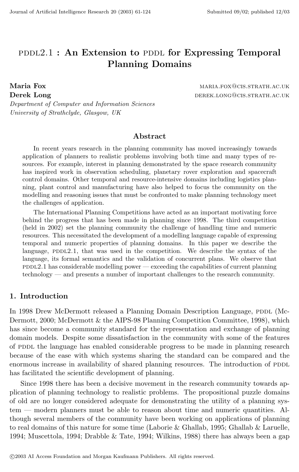
Cover for PDDL2.1: An Extension to PDDL for Expressing Temporal Planning Domains

Abstract

In recent years research in the planning community has moved increasingly towards application of planners to realistic problems involving both time and many types of resources. For example, interest in planning demonstrated by the space research community has inspired work in observation scheduling, planetary rover exploration and spacecraft control domains. Other temporal and resource-intensive domains including logistics planning, plant control and manufacturing have also helped to focus the community on the modelling and reasoning issues that must be confronted to make planning technology meet the challenges of application.

The International Planning Competitions have acted as an important motivating force behind the progress that has been made in planning since 1998. The third competition (held in 2002) set the planning community the challenge of handling time and numeric resources. This necessitated the development of a modelling language capable of expressing temporal and numeric properties of planning domains. In this paper we describe the language, PDDL2.1, that was used in the competition. We describe the syntax of the language, its formal semantics and the validation of concurrent plans. We observe that PDDL2.1 has considerable modelling power — exceeding the capabilities of current planning technology — and presents a number of important challenges to the research community.

Topics

formal semantics low earth orbits modeling languages reasoning validation logistics system

Keywords

PDDL2.1 temporal planning domains Domain Description Language temporal planning temporal reasoning frameworks classical planning temporal constraints plan metrics action schemas formal semantics

1. Introduction
2. PDDL Background
3. Numeric Expressions, Conditions and Effects
4. Plan Metrics
5. Durative Actions
5.1 The Interpretation of Concurrent plans
5.2 Numeric Change within Discretised Durative Actions
5.3 Durative Actions with Continuous Effects
5.4 Related Approaches
6. Introduction to the Semantics of PDDL2.1
7. The Semantics of Simple Plans
7.1 Semantics of a Simple Plan
8. The Semantics of Durative Actions
8.1 Durative Actions with Conditional Effects
9. The Semantics of Continuous Durative Actions
10. Plan Validation
11. Related Work: Representing and Reasoning about Time
11.1 Continuous change
11.2 Concurrency
11.3 Temporal extent
11.4 Planning with Time
12. Conclusions
Acknowledgements
Appendix A. BNF Specification of PDDL2.1
A.1 Domains
A.2 Actions
A.3 Durative Actions
A.4 Problems
A.5 Requirements
References

Knowls

Knowl 1 — Expressive Levels of PDDL2.1
definition
PDDL2.1 organizes temporal and metric planning expressiveness into nested levels of language capabilities:
- Level 1 (Classical/ADL): Supports STRIPS and ADL constructs, including typed variables, negative preconditions, disjunctive preconditions, equality predicates, existential and universal quantifiers, and conditional effects.
- Level 2 (Numeric Extensions): Introduces primitive numeric expressions (numeric fluents) mapping tuples of objects to real values ( $Fs: \text{Object}^n \to \mathbb{R}$ ), arithmetic preconditions using comparisons ( $=, <, >, \le, \ge$ ), numeric update operators (assign, increase, decrease, scale-up, scale-down), and problem-level plan optimization metrics (:metric minimize / maximize).
- Level 3 (Discretised Durative Actions): Adds durative action schemas characterized by explicit duration constraints and temporally annotated conditions (at start, over all, at end) and discrete effects (at start, at end), where logical changes and step-function numeric updates occur strictly at the action end points.
- Level 4 (Continuous Durative Actions): Extends durative actions with continuous numeric effects parameterized by the local elapsed-time continuous fluent #t (representing rates of change $\frac{df}{dt} = g$ ), enabling continuous resource consumption, production, and trajectory evaluation over action intervals.
Level 5 (defined in companion literature) further extends Level 4 with spontaneous exogenous events and continuous physical processes.
Knowl 2 — Planning Instance and Extended State in PDDL2.1
definition
A simple planning instance in PDDL2.1 is defined as a pair $I = (Dom, Prob)$ , where:
- $Dom = (Fs, Rs, As, \text{arity})$ consists of finite sets of function symbols $Fs$ , relation symbols $Rs$ , action schemas $As$ , and a signature mapping $\text{arity}$ .
- $Prob = (Os, \text{Init}, G)$ consists of domain objects $Os$ , an initial state specification $\text{Init}$ , and a goal condition $G$ .
The set of primitive numeric expressions ( $PNEs$ ) comprises all terms formed by applying domain function symbols $Fs$ to objects in $Os$ . The dimension $\text{dim} = |PNEs|$ is the total number of distinct primitive numeric expressions in $I$ . The set of atoms $Atms$ consists of all ground atomic propositions formed by applying relation symbols $Rs$ to objects $Os$ .

Let $\mathbb{R}_\bot = \mathbb{R} \cup \{\bot\}$ , where $\bot$ denotes an undefined value. A state $S$ is defined as a 3-tuple: $S \in (\mathbb{R} \times \mathcal{P}(Atms) \times \mathbb{R}_\bot^{\text{dim}})$ where:
1. The first element $t \in \mathbb{R}$ is the state timestamp.
2. The second element $s \subseteq Atms$ is the logical state (the set of true propositions under the Closed World Assumption).
3. The third element $\mathbf{x} \in \mathbb{R}_\bot^{\text{dim}}$ is a vector containing the values of the $\text{dim}$ primitive numeric expressions in $I$ .
The initial state is $(0, \text{Init}_{\text{logical}}, \mathbf{x}_0)$ , where $\mathbf{x}_0$ contains the initial values defined in $\text{Init}_{\text{numeric}}$ (and $\bot$ for any unassigned expressions).
Knowl 3 — Numeric Effects and State Updating Function
definition
In PDDL2.1, a numeric effect has the syntactic form $(\text{op}\; l\; r)$ , where $\text{op} \in \{\text{assign}, \text{increase}, \text{decrease}, \text{scale-up}, \text{scale-down}\}$ , $l$ is a primitive numeric expression (the lvalue), and $r$ is an arithmetic expression over numbers and primitive numeric expressions (the rvalue).

Each numeric effect is normalized into an assignment proposition $(= l' \; \text{expr})$ , where $l'$ represents the updated value of $l$ in the post-action state and $\text{expr}$ is an arithmetic formula evaluated on pre-action values (for example, $(\text{increase}\; p\; q)$ becomes $(= p' \; (+ \; p \; q))$ ).

A ground action $a$ is defined as valid if no primitive numeric expression appears as an lvalue in more than one simple assignment effect, or in more than one distinct type of assignment effect within $a$ .

For a valid ground action $a$ with assignment propositions $NP_a$ , the numeric state update is the composition of numeric projection functions $\{NPF_p : \mathbb{R}_\bot^{\text{dim}} \to \mathbb{R}_\bot^{\text{dim}} \mid p \in NP_a\}$ , where each $NPF_p(\mathbf{x}) = \mathbf{x}'$ modifies the coordinate corresponding to the lvalue of $p$ according to its assignment rule while leaving all other coordinates unaltered ( $x'_i = x_i$ for all $i \neq \text{index}(l)$ ). Because non-conflicting and additive updates commute, the composite function is well-defined and order-independent.
Knowl 4 — Action Non-Interference and Mutual Exclusion Conditions
definition
In PDDL2.1, two concurrent ground actions $a$ and $b$ are non-interfering (non-mutex) if and only if all of the following four conditions hold:
1. $GPre_a \cap (Add_b \cup Del_b) = \emptyset$ and $GPre_b \cap (Add_a \cup Del_a) = \emptyset$
2. $Add_a \cap Del_b = \emptyset$ and $Add_b \cap Del_a = \emptyset$
3. $L_a \cap R_b = \emptyset$ and $R_a \cap L_b = \emptyset$
4. $L_a \cap L_b \subseteq L^*_a \cap L^*_b$
where:
- $GPre_a$ is the set of ground logical atoms in the precondition of $a$ .
- $Add_a$ and $Del_a$ are the sets of ground atoms added and deleted by $a$ , respectively.
- $L_a$ is the set of primitive numeric expressions appearing as lvalues in $a$ .
- $R_a$ is the set of primitive numeric expressions read by $a$ (appearing in action preconditions or within rvalue expressions in action effects).
- $L^*_a \subseteq L_a$ is the subset of lvalues modified exclusively via additive operators (increase or decrease).
If any condition is violated, $a$ and $b$ are mutually exclusive (mutex). This rule embodies the "no moving targets" principle: simultaneous actions cannot read a state component that another concurrent action modifies, and concurrent writes to the same numeric fluent are valid if and only if both actions perform additive updates.
Knowl 5 — Happening Execution and Simple Plan Semantics
model/method
In PDDL2.1, a simple plan $SP$ is a finite collection of timed simple actions $(t, a)$ , where $t \in \mathbb{Q}^+$ is a positive rational timestamp and $a$ is an instantiated action name.

The happening sequence $\{t_i\}_{i=0\dots k}$ of $SP$ is the strictly increasing ordered sequence of all unique timestamps appearing in $SP$ . The happening $E_t$ at time $t$ is the set of action names scheduled at time $t$ .

The execution of a happening $H$ scheduled at time $t_H$ in state $(t, s, \mathbf{x})$ is defined as follows:
1. The set of applicable ground actions is $A_H = \{a \mid \text{name}(a) \in H, a \text{ is valid}, \text{and } Pre_a \text{ is satisfied in } (t, s, \mathbf{x})\}$ .
2. Execution is undefined if $|A_H| \neq |H|$ or if any pair of actions in $A_H$ is mutex.
3. Otherwise, the resulting state is $(t_H, s', \mathbf{x}')$ , where: $s' = \left(s \setminus \bigcup_{a \in A_H} Del_a\right) \cup \bigcup_{a \in A_H} Add_a$ and $\mathbf{x}'$ is obtained by applying the composite updating functions $\{NPF_a \mid a \in A_H\}$ to $\mathbf{x}$ .
A simple plan $SP$ is executable if, starting from $S_0 = (0, \text{Init}_{\text{logical}}, \mathbf{x}_0)$ , each successive happening $E_{t_i}$ transitions $S_i$ to $S_{i+1}$ , producing a unique trace $\{S_0, S_1, \dots, S_{k+1}\}$ . $SP$ is valid if it is executable and the final state $S_{k+1}$ satisfies goal $G$ .
Knowl 6 — Compilation and Semantics of Discretised Durative Actions
model/method
In PDDL2.1, a discretised durative action instance is specified as $(t, a[d])$ , where $t \in \mathbb{Q}^+$ is the start time, $d \in \mathbb{Q}^{\ge 0}$ is the duration, and conditions/effects are temporally annotated (at start, over all, at end).

Each ground durative action schema $DA$ is decomposed into three instantaneous simple actions:
1. $DA_{\text{start}}$ : Precondition is $\bigwedge \{p \mid (\text{at start } p) \in DA\} \wedge DC_{\text{start}}^{DA}$ ; Effect is $\bigwedge \{e \mid (\text{at start } e) \in DA\}$ .
2. $DA_{\text{end}}$ : Precondition is $\bigwedge \{p \mid (\text{at end } p) \in DA\} \wedge DC_{\text{end}}^{DA}$ ; Effect is $\bigwedge \{e \mid (\text{at end } e) \in DA\}$ .
3. $DA_{\text{inv}}$ : Precondition is $\bigwedge \{p \mid (\text{over all } p) \in DA\}$ ; Effect is empty $\emptyset$ .
Here $DC_{\text{start}}^{DA}$ and $DC_{\text{end}}^{DA}$ denote the action duration constraints evaluated at start and end, respectively.

Given a temporal plan $P$ , its happening sequence $\{t_i\}_{i=0\dots k}$ contains all start times $t$ and end times $t+d$ . The induced simple plan $\text{simplify}(P)$ is formed by:
- Adding $(t, a)$ for each instantaneous action $(t, a) \in P$ .
- Adding $(t, DA_{\text{start}}[?\text{duration} := d])$ and $(t+d, DA_{\text{end}}[?\text{duration} := d])$ for each durative action $(t, a[d]) \in P$ .
- Inserting invariant checking actions $\left(\frac{t_i + t_{i+1}}{2}, DA_{\text{inv}}\right)$ for every pair of consecutive happenings $t_i, t_{i+1}$ within the execution interval $[t, t+d]$ .
The durative plan $P$ is executable and valid if and only if its induced simple plan $\text{simplify}(P)$ is executable and valid.
Knowl 7 — Compilation of Durative Conditional Effects via Memory Propositions
model/method
When a PDDL2.1 durative action contains conditional effects spanning time points—such as: $(\text{when } (\text{and } (\text{at start } p_s)\; (\text{over all } p_i)\; (\text{at end } p_e))\; (\text{at end } q))$ the condition cannot be evaluated from the end state alone because state transitions lack execution history. The PDDL2.1 semantics compiles such conditional effects into instantaneous actions by introducing unique propositional memory fluents:
1. $M_{p_s}$ : A fresh proposition asserting that start condition $p_s$ was satisfied at action initiation.
2. $M_{p_i}$ : A fresh proposition asserting that invariant condition $p_i$ has remained continuously true throughout the action execution interval.
The action transformation proceeds as follows:
- $DA_{\text{start}}$ receives the conditional effect $(\text{when } p_s \; M_{p_s})$ and unconditionally adds $M_{p_i}$ .
- At every midpoint happening $\frac{t_j + t_{j+1}}{2}$ within the action interval, an invariant-monitoring action is inserted with the effect: $(\text{when } (\text{and } M_{p_i} \; (\text{not } p_i)) \; (\text{not } M_{p_i}))$ which deletes $M_{p_i}$ permanently if $p_i$ is violated at any point.
- $DA_{\text{end}}$ receives the conditional effect: $(\text{when } (\text{and } M_{p_s} \; M_{p_i} \; p_e) \; q)$
This ensures that delayed conditional effects execute at the action termination if and only if all start, invariant, and end conditions held at their respective times.
Knowl 8 — Semantics and Invariant Safety of Continuous Durative Actions
definition
In PDDL2.1 Level 4, continuous durative actions contain continuous numeric effects of the form $(\text{increase } p \; (* \; \#t \; q))$ or $(\text{decrease } p \; (* \; \#t \; q))$ , where $\#t$ represents local elapsed action time.

An induced continuous plan is a triple $(S, Invs, Cts)$ , where $S = \text{simplify}(P)$ , $Invs = \{(Q, t, t+d) \mid (t, a[d]) \in P \text{ and } (\text{over all } Q) \in a\}$ , and $Cts$ contains active continuous effect systems over each happening interval $(t_i, t_{i+1})$ .
1. Continuous Update Function: Over each open interval $(t_i, t_{i+1})$ , the set of active continuous effects $C$ defines a system of differential equations $\frac{df_C}{dt} = g$ with initial condition $f_C(0) = \mathbf{x}_i$ , where $\mathbf{x}_i$ is the numeric state vector at $t_i$ .
2. Continuous Trace: The state immediately preceding the discrete happening at $t_{i+1}$ is $T_i = (t_{i+1}, s_i, f_C(t_{i+1} - t_i))$ , where $s_i$ is the invariant logical state over $(t_i, t_{i+1})$ . The discrete happening $E_{t_{i+1}}$ is then applied to $T_i$ to yield state $S_{i+1}$ .
3. Invariant Safety: Plan $P$ is invariant safe if and only if for every active continuous update function $f_i$ over interval $I = (t_i, t_{i+1})$ and every invariant $(Q, t, u) \in Invs$ such that $I \subseteq (t, u)$ : $\forall \tau \in I, \quad \text{Num}(s_i, Q)(f_i(\tau)) = \text{true}$
A continuous plan $P$ is executable if its continuous trace is defined and it is invariant safe, and valid if the final state $S_{k+1}$ satisfies the goal specification $G$ .
Knowl 9 — PDDL2.1 Plan Metric Specifications
model/method
PDDL2.1 extends problem definitions with an optional :metric field to evaluate plan quality: (:metric <optimization> <ground-f-exp>) where <optimization> is either minimize or maximize, and <ground-f-exp> is an arithmetic expression over numeric fluents, constants, and the reserved fluent total-time.

Key characteristics include:
- total-time evaluates to the temporal span (makespan) of the entire plan.
- State-dependent optimization requires explicit domain instrumentation: fluents tracking resource consumption (such as total fuel or energy consumed) must be initialized in :init and explicitly updated by action effects.
- Metric expressions are not required to be linear and can combine makespan with domain fluents, for example: (:metric minimize (+ (* 2 (fuel-used car)) total-time))
Knowl 10 — Decidability and Complexity of Plan Validation versus Planning
theoretical result
In PDDL2.1, planning search and plan validation possess fundamentally different computational complexities:
- Planning Undecidability: The planning problem in PDDL2.1 with numeric fluents (Level 2 and above) is undecidable. Furthermore, determining whether a numeric planning problem with an optimization metric is well-defined (i.e., whether unbounded action loops can generate arbitrarily high utility) is undecidable.
- Plan Validation Decidability: Plan validation for a specified plan in PDDL2.1 is decidable across all levels, including discretized durative actions, actions with duration inequalities, and continuous durative actions with linear/quadratic continuous dynamics. Because actions and durations are fully grounded and scheduled in the candidate plan, the induced sequence of happenings is finite.
- Validation Tractability: Validation is polynomial-time tractable for discrete and discretized durative plans (Levels 1–3). For continuous durative plans (Level 4), validation remains polynomial-time tractable provided continuous effects and invariant conditions are restricted to linear or low-degree polynomial functions of time without coupled non-linear differential equations.
Knowl 11 — Non-Zero Temporal Separation and Pragmatic Plan Validation
assumption
PDDL2.1 formalizes the relationship between theoretical continuous-time semantics and real-world execution through an $\epsilon$ -separation tolerance principle:
1. $\epsilon$ -Separation of Mutex Endpoints: Physical execution architectures cannot guarantee infinitely precise simultaneity of independently triggered events. Therefore, two action endpoints that are mutually exclusive (mutex) cannot occur at the exact same timestamp; they must be separated by a minimum non-zero duration $\Delta t \ge \epsilon > 0$ . Non-mutex endpoints may be scheduled at the exact same instant.
2. Floating-Point Pragmatic Validation: Planners represent time stamps and numeric quantities as finite-precision floating-point numbers rather than arbitrary-precision algebraic expressions. Automated validators evaluate numeric conditions, duration constraints, and invariant boundaries with respect to a defined tolerance $\epsilon > 0$ . The tolerance $\epsilon$ serves simultaneously as the numeric boundary threshold and the minimum temporal buffer between conflicting events.

Coverage note — PDDL2.1 BNF grammar details from the appendix and comparisons to specific historical planners (such as TGP, Zeno, IxTeT, and Sapa) were omitted as they either represent concrete syntax specifications or background context.

References

1.Allen, J. (1984). Towards a general theory of action and time. Artificial Intelligence, 23, 123–154.
2.Allen, J. (1991). Planning as temporal reasoning. In Proceedings of KR-91, pp. 3–14.
3.Bacchus, F., & Ady, M. (2001). Planning with resources and concurrency: A forward chaining approach. In Proceedings of IJCAI’01, pp. 417–424.
4.Bacchus, F., & Kabanza, F. (1998). Planning for temporally extended goals. Annals of Mathematics and Artificial Intelligence, 22, 5–27.
5.Bacchus, F., & Kabanza, F. (2000). Using temporal logic to express search control knowledge for planning. Artificial Intelligence, 116(1-2), 123–191.
6.Bacchus, F., Tenenberg, J., & Koomen, J. (1991). A non-reified temporal logic for AI. Artificial Intelligence, 52, 87–108.
7.Blum, A., & Furst, M. (1995). Fast Planning through Plan-graph Analysis. In Proceedings of IJCAI-95.
8.Cesta, A., & Oddi, A. (1996). Gaining efficiency and flexibility in the simple temporal problem. In Chittaro, L., Goodwin, S., Hamilton, H., & Montanari, A. (Eds.), Proceedings of TIME’96.
9.Chapman, D. (1987). Planning for conjunctive goals. Artificial Intelligence, 29, 333–377.
10.Dechter, R., Meiri, I., & Pearl, J. (1991). Temporal constraint networks. Artificial Intelligence, 49.
11.Do, M. B., & Kambhampati, S. (2001). Sapa: a domain-independent heuristic metric temporal planner. In Proceedings of ECP-01.
12.Drabble, B., & Tate, A. (1994). The use of optimistic and pessimistic resource profiles to inform search in an activity based planner. In Proceedings of AIPS-94. AAAI Press.
13.El-Kholy, A., & Richards, B. (1996). Temporal and resource reasoning in planning: the ParcPlan approach. In Proceedings of ECAI’96.
14.Fikes, R., & Nilsson, N. (1971). STRIPS: A new approach to the application of theorem-proving to problem-solving. Artificial Intelligence, 2(3), 189–208.
15.Fox, M., & Long, D. (2002). PDDL+ : Planning with time and metric resources. Tech. rep. Department of Computer Science, 21/02, University of Durham, UK. Available at: http://www.dur.ac.uk/d.p.long/competition.html.
16.Galipienso, M., & Sanchis, F. (2002). Representation and reasoning with disjunction temporal constraints. In Proceedings of TIME’02.
17.Garrido, A., Onaind´ıa, E., & Barber, F. (2001). Time-optimal planning in temporal problems. In Proceedings of ECP’01.
18.Gazen, B., & Knoblock, C. (1997). Combining the expressivity of UCPOP with the efficiency of Graphplan. In Proceedings of ECP-97, pp. 221–233.
19.Gelfond, M., Lifschitz, V., & Rabinov, A. (1991). What are the limitations of the situation calculus?. In Boyer, R. (Ed.), Essays in honor of Woody Bledsoe, pp. 167–179. Kluwer Academic.
20.Ghallab, M., & Laruelle, H. (1994). Representation and control in IxTeT, a temporal planner. In Proceedings of AIPS’94.
21.Gupta, V., Henziner, T., & Jagadeesan, R. (1997). Robust timed automata. In HART-97: Hybrid and Real-time Systems, LNCS 1201, pp. 331–345. Springer-Verlag.
22.Haslum, P., & Geffner, H. (2001). Heuristic planning with time and resources. In Proceedings of ECP’01, Toledo.
23.Hayes, P., & Allen, J. (1987). Short time periods. In Proceedings of IJCAI-87, pp. 981–983.
24.Helmert, M. (2002). Decidability and undecidability results for planning with numerical state variables. In Proceedings of AIPS-02.
25.Henzinger, T. (1996). The theory of hybrid automata. In Proceedings of the 11th Annual Symposium on Logic in Computer Science. Invited tutorial., pp. 278–292. IEEE Computer Society Press.
26.Henzinger, T., & Raskin, J.-F. (2000). Robust undecidability of timed and hybrid systems. In Proceedings of the 3rd International Workshop on Hybrid Systems: Computation and Control. LNCS 1790., pp. 145–159. Springer-Verlag.
27.Howey, R., & Long, D. (2002). Validating plans with continuous effects. Tech. rep., Dept. Computer Science, University of Durham.
28.Jonsson, A., Morris, P., Muscettola, N., & Rajan, K. (2000). Planning in interplanetary space: theory and practice. In Proceedings of AIPS-00.
29.Kowalski, R., & Sergot, M. (1986). A logic-based calculus of events. New Generation Computing, 4, 67–95.
30.Laborie, P., & Ghallab, M. (1995). Planning with sharable resource constraints. In Proceedings of IJCAI-95. Morgan Kaufmann.
31.Lifschitz, E. (1986). On the semantics of STRIPS. In Proceedings of 1986 Workshop: Reasoning about Actions and Plans.
32.Long, D., & Fox, M. (2003a). Exploiting a graphplan framework in temporal planning. In Proceedings of ICAPS’03.
33.Long, D., & Fox, M. (2003b). An overview and analysis of the results of the 3rd International Planning Competition. Journal of Artifical Intelligence Research, this issue.
34.McAllester, D., & Rosenblitt, D. (1991). Systematic nonlinear planning. In Proceedings of AAAI’91, Vol. 2, pp. 634–639, Anaheim, California, USA. AAAI Press/MIT Press.
35.McCarthy, J. (1980). Circumscription — a form of non-monotonic reasoning. Artificial Intelligence, 13, 27–39.
36.McCarthy, J., & Hayes, P. (1969). Some philosophical problems from the standpoint of artificial intelligence. In Meltzer, B., & Michie, D. (Eds.), Machine Intelligence 4, pp. 463–502. Edinburgh University Press.
37.McDermott, D. (1982). A temporal logic for reasoning about processes and plans. Cognitive Science, 6, 101–155.
38.McDermott, D. (2000). The 1998 AI planning systems competition. AI Magazine, 21(2).
39.McDermott, D. (2003). Reasoning about autonomous processes in an estimated-regression planner. In Proceedings of ICAPS-03.
40.McDermott, D., & the AIPS-98 Planning Competition Committee (1998). PDDL–the planning domain definition language. Tech. rep., Available at: www.cs.yale.edu/homes/dvm.
41.Muscettola, N. (1994). HSTS: Integrating planning and scheduling. In Zweben, M., & Fox, M. (Eds.), Intelligent Scheduling, pp. 169–212. Morgan Kaufmann, San Mateo, CA.
42.Nau, D., Cao, Y., Lotem, A., & Mu˜noz-Avila, H. (1999). SHOP: Simple hierarchical ordered planner. In Proceedings of IJCAI’99.
43.Pednault, E. (1986). Formulating multiagent, dynamic-world problems in the classical planning framework. In Georgeff, M., & Lansky, A. (Eds.), Proceedings of the Timberline Oregon Workshop on Reasoning about Actions and Plans.
44.Pednault, E. (1989). ADL: Exploring the middle ground between STRIPS and the situation calculus. In Proceedings of KR-89, pp. 324–332.
45.Penberthy, J., & Weld, D. (1994). Temporal planning with continuous change. In Proceedings of AAAI-94. AAAI/MIT Press.
46.Penberthy, J., & Weld, D. (1992). UCPOP: a sound, complete, partial-order planner for ADL. In Proceedings of KR’92, pp. 103–114, Los Altos, CA. Kaufmann.
47.Rabideau, G., Knight, R., Chien, S., Fukunaga, A., & Govindjee, A. (1999). Iterative repair planning for spacecraft operations in the ASPEN system. In International Symposium on Artificial Intelligence Robotics and Automation in Space (i-SAIRAS).
48.Reichgelt, H. (1989). A comparison of first order and modal theories of time. In Jackson, P., Reichgelt, H., & van Harmelen, F. (Eds.), Logic-based knowledge representation, pp. 143–176. MIT Press.
49.Reiter, R. (1980). A logic for default reasoning. Artificial Intelligence, 13, 81–132.
50.Russell, S., & Norvig, P. (1995). Artificial Intelligence: a Modern Approach. Prentice Hall.
51.Sandewall, E. (1994). Features and fluents: the representation of knowledge about dynamical systems, volume I. Oxford University Press.
52.Shanahan, M. (1990). Representing continuous change in the event calculus. In Proceedings of ECAI’90, pp. 598–603.
53.Shanahan, M. (1999). The event calculus explained. In Wooldridge, M., & Veloso, M. (Eds.), Artificial Intelligence Today, pp. 409–430. Springer Lecture Notes in Artificial Intelligence no. 1600.
54.Shoham, Y. (1985). Ten requirements for a theory of change. New Generation Computing, 3, 467–477.
55.Smith, D., & Weld, D. (1999). Temporal planning with mutual exclusion reasoning. In Proceedings of IJCAI-99, Stockholm, pp. 326–337.
56.Tate, A. (1977). Generating project networks. In Proceedings of IJCAI’77.
57.van Bentham, J. (1983). The logic of time. Kluwer Academic Press, Dordrecht.
58.Vere, S. (1983). Planning in time: Windows and durations for activities and goals. IEEE Transactions on Pattern Analysis and Machine Intelligence, 5.
59.Vila, L. (1994). A survey on temporal reasoning in artificial intelligence. AI Communications, 7, 4–28.
60.Wilkins, D. (1988). Practical Planning: Extending the Classical AI Planning Paradigm. Morgan Kaufmann Publishers Inc., San Francisco, CA.

Citation

MLA

Fox, M., and D. Long. “PDDL2.1: An Extension to PDDL for Expressing Temporal Planning Domains”. Journal of Artificial Intelligence Research, vol. 20, 2003, pp. 61–124, https://doi.org/10.1613/jair.1129.

APA

Fox, M., & Long, D. (2003). PDDL2.1: An Extension to PDDL for Expressing Temporal Planning Domains. Journal of Artificial Intelligence Research, 20, 61–124. https://doi.org/10.1613/jair.1129

Chicago

Fox, M., and D. Long. 2003. “PDDL2.1: An Extension to PDDL for Expressing Temporal Planning Domains”. Journal of Artificial Intelligence Research 20: 61–124. https://doi.org/10.1613/jair.1129.

Harvard

Fox, M. and Long, D. (2003) “PDDL2.1: An Extension to PDDL for Expressing Temporal Planning Domains”, Journal of Artificial Intelligence Research, 20, pp. 61–124. Available at: https://doi.org/10.1613/jair.1129.

Vancouver

1. Fox M, Long D (2003) PDDL2.1: An Extension to PDDL for Expressing Temporal Planning Domains. Journal of Artificial Intelligence Research 20:61–124

BibTeX

@article{Fox_2003, title={PDDL2.1: An Extension to PDDL for Expressing Temporal Planning Domains}, volume={20}, ISSN={1076-9757}, url={http://dx.doi.org/10.1613/jair.1129}, DOI={10.1613/jair.1129}, journal={Journal of Artificial Intelligence Research}, publisher={AI Access Foundation}, author={Fox, M. and Long, D.}, year={2003}, month=Dec, pages={61–124} }

Metadata:Crossref

Source Code

This paper has an official code repository available. Click below to access the source code.

View Repository

Access the Paper

This paper is available from its original source. Click below to access the PDF.

Open PDF

License: https://creativecommons.org/licenses/by/4.0/

PDDL2.1: An Extension to PDDL for Expressing Temporal Planning Domains

Abstract

Topics

Keywords

Table of Contents

Knowls

Knowl 1 — Expressive Levels of PDDL2.1

Knowl 2 — Planning Instance and Extended State in PDDL2.1

Knowl 3 — Numeric Effects and State Updating Function

Knowl 4 — Action Non-Interference and Mutual Exclusion Conditions

Knowl 5 — Happening Execution and Simple Plan Semantics

Knowl 6 — Compilation and Semantics of Discretised Durative Actions

Knowl 7 — Compilation of Durative Conditional Effects via Memory Propositions

Knowl 8 — Semantics and Invariant Safety of Continuous Durative Actions

Knowl 9 — PDDL2.1 Plan Metric Specifications

Knowl 10 — Decidability and Complexity of Plan Validation versus Planning

Knowl 11 — Non-Zero Temporal Separation and Pragmatic Plan Validation

References

Citation

BibTeX

Source Code

Access the Paper