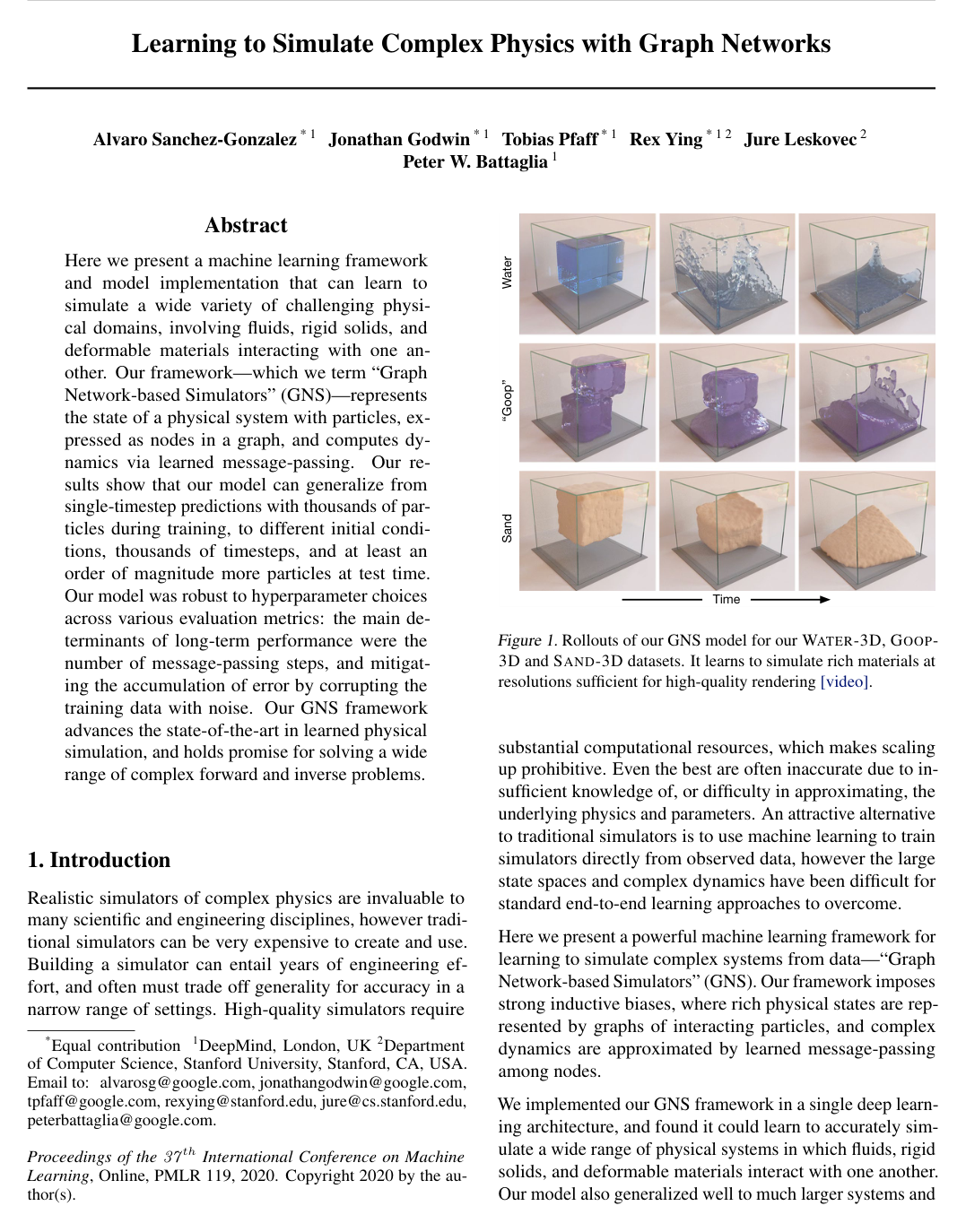
Learning to Simulate Complex Physics with Graph Networks

Alvaro Sanchez-GonzalezJonathan GodwinTobias PfaffRex YingJure LeskovecPeter W. Battaglia

article2020ICML1,624 citations

Develops a particle-based graph network simulator capable of learning complex physical dynamics across fluids, rigid solids, and deformable materials, successfully generalizing over thousands of timesteps and scaling to an order of magnitude more particles at test time.

Listen

Traditional computer simulators for complex physics—such as fluids, rigid solids, and deformable materials—are critical for engineering and scientific analysis but often require years of manual engineering, demand massive computing power, and struggle to generalize across diverse material types. Machine learning offers an alternative by learning dynamics directly from data, yet previous machine learning simulators were typically specialized for narrow tasks, relied on rigid domain-specific assumptions, and struggled to scale over long trajectories without accumulating catastrophic errors.

The article demonstrates a unified machine learning framework called Graph Network-based Simulators (GNS) that learns to simulate a wide variety of interacting physical materials. The primary objective is to evaluate whether a single, general deep learning architecture can accurately model multi-material dynamics, prevent compounding rollout errors, and generalize to significantly larger systems and longer timeframes than seen during training.

The researchers formulated physical simulation as learned message-passing on particle graphs. The architecture embeds particles as nodes and local spatial relations as edges, computes interactions across multiple message-passing steps, and predicts per-particle accelerations that update positions over time. Credibility was established by evaluating the model across more than a dozen distinct 2D and 3D simulation datasets generated by standard physics engines, spanning chaotic fluids, granular sand, viscous deformable substances, and rigid obstacles. Training relied on one-step prediction pairs perturbed with random-walk noise to expose the network to non-ideal inputs, with benchmarks measuring one-step error, long-horizon trajectory error, and distributional discrepancies.

The analysis yielded several vital findings. First, a single GNS architecture accurately simulated diverse single- and multi-material systems over thousands of steps, maintaining stability across up to 20,000 particles in training. Second, the model demonstrated substantial zero-shot generalization; when trained on small domains with approximately 2,500 particles, it successfully predicted dynamics in test domains with up to 85,000 particles (a 34-fold increase), areas 32 times larger, and trajectories up to 8 times longer. Third, systematic ablations revealed that long-horizon accuracy depends heavily on unshared graph network parameters, larger connectivity radii, relative position encodings, and noise injection during training, while other hyperparameters had minimal effect. Finally, GNS outperformed leading domain-specific machine learning baselines across all benchmarked datasets without requiring hand-crafted physical constraints.

These results demonstrate that organizations can replace specialized, bespoke simulation pipelines with a single, highly flexible machine learning architecture. Because the model operates on continuous particle dynamics and supports gradient backpropagation, it significantly reduces the engineering time required to build custom simulators while opening opportunities for solving complex inverse problems and design optimization. The approach delivers inference runtimes broadly comparable to CPU-based ground truth physics engines, while shifting the computational burden toward highly parallelizable graph operations.

Decision-makers considering learned simulation pipelines should adopt the core architectural principles identified in the article—specifically relative spatial encodings, multi-step message-passing, and random-walk training noise. Before deployment in production settings, technical teams should conduct pilot studies to optimize graph neighborhood computation, which accounted for the majority of execution runtime. Further validation is also recommended to explore incorporating generic physical constraints, such as energy and momentum conservation, directly into the network.

Readers should note specific operational boundaries and maintain appropriate caution. The article notes failure modes under extreme conditions: rigid shapes can slowly deform over very long rollouts (e.g., 1,500 steps) during violent shaking, and complex contact phenomena like static adhesion may be mispredicted if underrepresented in training data. Nevertheless, confidence remains high in the model's core capability to robustly simulate and generalize complex particle interactions across diverse physical domains.

  • Paper: Relational inductive biases, deep learning, and graph networks, Peter W. Battaglia et al. (2018). This foundational paper establishes the Graph Network framework and relational inductive biases that directly form the architectural backbone of the Graph Network-based Simulators.
  • Paper: Interaction Networks for Learning about Objects, Relations and Physics, Peter W. Battaglia et al. (2016). This work introduces Interaction Networks for learning object relations and physical dynamics on graphs, providing the foundational conceptual paradigm for learning particle-based physics simulations.
  • Paper: The Graph Neural Network Model, Franco Scarselli et al. (2009). This seminal paper defines the original Graph Neural Network model and its information diffusion mechanisms that underpin modern message-passing architectures.
  • Paper: Graph Neural Networks: A Review of Methods and Applications, Jie Zhou et al. (2018). This comprehensive review categorizes spatial and spectral graph neural network formulations and message-passing schemes utilized in learned physical models.
  • Paper: How Powerful are Graph Neural Networks?, Keyulu Xu et al. (2019). This paper analyzes the expressive limits of message-passing aggregation in graph neural networks, explaining the necessity of multi-step message passing in physical simulation.
Cover for Learning to Simulate Complex Physics with Graph Networks

Abstract

Here we present a machine learning framework and model implementation that can learn to simulate a wide variety of challenging physical domains, involving fluids, rigid solids, and deformable materials interacting with one another. Our framework---which we term "Graph Network-based Simulators" (GNS)---represents the state of a physical system with particles, expressed as nodes in a graph, and computes dynamics via learned message-passing. Our results show that our model can generalize from single-timestep predictions with thousands of particles during training, to different initial conditions, thousands of timesteps, and at least an order of magnitude more particles at test time. Our model was robust to hyperparameter choices across various evaluation metrics: the main determinants of long-term performance were the number of message-passing steps, and mitigating the accumulation of error by corrupting the training data with noise. Our GNS framework advances the state-of-the-art in learned physical simulation, and holds promise for solving a wide range of complex forward and inverse problems.

Table of Contents

  • 1 Introduction
  • 2 Related Work
  • 3 GNS Model Framework
  • 3.1 General Learnable Simulation
  • 3.2 Simulation as Message-Passing on a Graph
  • 4 Experimental Methods
  • 4.1 Physical Domains
  • 4.2 GNS Implementation Details
  • 4.3 Training
  • 4.4 Evaluation
  • 5 Results
  • 5.1 Simulating Complex Materials
  • 5.2 Multiple Interacting Materials
  • 5.3 Generalization
  • 5.4 Key Architectural Choices
  • 5.5 Comparisons to Previous Models
  • 6 Conclusion
  • References
  • A Supplementary GNS Model Details
  • B Supplementary Experimental Methods
  • B.1 Physical Domains
  • B.2 Implementation Details
  • B.3 Training
  • B.4 Distributional Evaluation Metrics
  • C Supplementary Results
  • C.1 Architectural Choices with Minor Impact on Performance
  • C.2 Noise-Related Training Parameters
  • C.3 Distributional Evaluation Metrics
  • C.4 Quantitative Results on all Datasets
  • C.5 Quantitative Generalization Results on Continuous Domain
  • C.6 Inference Times
  • C.7 Example Failure Cases
  • D Supplementary Baseline Comparisons
  • D.1 Continuous Convolution (CConv)
  • D.2 DPI

Knowls

  1. Knowl 1 — GNS Architecture and Encode-Process-Decode Pipeline

    model/method

    The Graph Network-based Simulator (GNS) is a general learned physical simulation model that maps particle states to physical dynamics via message passing over interaction graphs. The model operates under an Encode-Process-Decode framework:

    1. Input Representation: For a system of NN particles in DD spatial dimensions (D∈{2,3}D \in \{2, 3\}), each particle ii at time step tkt_k is represented by a feature vector: xitk=[pitk,p˙itk−C+1,…,p˙itk,ai]x_i^{t_k} = [p_i^{t_k}, \dot{p}_i^{t_k-C+1}, \dots, \dot{p}_i^{t_k}, a_i] where pitk∈RDp_i^{t_k} \in \mathbb{R}^D denotes particle position, the sequence (p˙itk−C+1,…,p˙itk)(\dot{p}_i^{t_k-C+1}, \dots, \dot{p}_i^{t_k}) denotes CC historical velocities (C=5C = 5) computed by first-order finite differences p˙it=pit−pit−1\dot{p}_i^t = p_i^t - p_i^{t-1}, and ai∈R16a_i \in \mathbb{R}^{16} is a learned embedding representing material type (e.g., water, sand, goop, rigid object, or boundary particle). For fixed orthogonal bounding walls, vector distances from particle ii to each wall are appended and clipped to a interaction radius RR.

    2. Encoder: Constructs an initial graph G0=(V,E)G^0 = (V, E) where nodes vi∈Vv_i \in V correspond to particles and directed edges eij∈Ee_{ij} \in E connect particle pairs with Euclidean separation ∥pitk−pjtk∥≤R\|p_i^{t_k} - p_j^{t_k}\| \le R. Node features are encoded into latent representations vi0∈R128v_i^0 \in \mathbb{R}^{128} via a node multilayer perceptron (MLP) εv\varepsilon^v that masks out absolute coordinates pitkp_i^{t_k} to enforce spatial translation invariance: vi0=εv([p˙itk−C+1:tk,ai,g])v_i^0 = \varepsilon^v([\dot{p}_i^{t_k-C+1:t_k}, a_i, g]) where gg denotes optional global property vectors (e.g., gravity, external forces). Edge features are computed via an edge MLP εe\varepsilon^e using relative displacements and distances: eij0=εe([(pitk−pjtk),∥pitk−pjtk∥])e_{ij}^0 = \varepsilon^e([(p_i^{t_k} - p_j^{t_k}), \|p_i^{t_k} - p_j^{t_k}\|])

    3. Processor: Applies MM message-passing steps (M=10M = 10) over the graph using unshared Graph Networks (GNs) without global latent updates. Each step m∈{0,…,M−1}m \in \{0, \dots, M-1\} computes residual edge and node updates: eijm+1=eijm+ϕme([vim,vjm,eijm])e_{ij}^{m+1} = e_{ij}^m + \phi_m^e([v_i^m, v_j^m, e_{ij}^m]) vim+1=vim+ϕmv([vim,∑j∈N(i)eijm+1])v_i^{m+1} = v_i^m + \phi_m^v\left(\left[v_i^m, \sum_{j \in \mathcal{N}(i)} e_{ij}^{m+1}\right]\right) where N(i)={j:(i,j)∈E}\mathcal{N}(i) = \{j : (i, j) \in E\}, and ϕme,ϕmv\phi_m^e, \phi_m^v are MLPs.

    4. Decoder: Maps the final node latent vectors viMv_i^M via a decoder MLP δv\delta^v to per-particle acceleration predictions: p¨^itk=δv(viM)∈RD\hat{\ddot{p}}_i^{t_k} = \delta^v(v_i^M) \in \mathbb{R}^D

    All internal MLPs consist of 2 hidden layers of width 128 with ReLU activations, followed by LayerNorm after each hidden layer. The decoder MLP outputs linearly.

  2. Knowl 2 — Random-Walk Velocity Noise Injection for Rollout Error Mitigation

    model/method

    Training a one-step simulator on uncorrupted ground-truth data leads to severe error accumulation during multi-step autoregressive rollouts because the simulator is exposed to out-of-distribution states created by its own accumulated prediction errors. GNS resolves this by corrupting the input historical velocities with random-walk noise during training while supervising the network to correct the noise.

    For each particle ii, spatial dimension, and historical step in the sequence of CC velocity inputs, independent noise samples are drawn from N(0,σv2I)\mathcal{N}(0, \sigma_v^2 I) with standard deviation σv=0.0003\sigma_v = 0.0003. Noise is accumulated as a random walk across time to match the temporal structure of rollout errors. The historical positions are adjusted consistently to satisfy p˙~it=p~it−p~it−1\tilde{\dot{p}}_i^t = \tilde{p}_i^t - \tilde{p}_i^{t-1}.

    The target acceleration p¨i,targettk\ddot{p}_{i, \text{target}}^{t_k} for training is adjusted by subtracting the total accumulated velocity noise ϵi,accumtk\epsilon_{i, \text{accum}}^{t_k} present at the most recent step tkt_k: p¨i,targettk=p¨i,cleantk−ϵi,accumtkΔt\ddot{p}_{i, \text{target}}^{t_k} = \ddot{p}_{i, \text{clean}}^{t_k} - \frac{\epsilon_{i, \text{accum}}^{t_k}}{\Delta t} where p¨i,cleantk=pitk+1−2pitk+pitk−1Δt2\ddot{p}_{i, \text{clean}}^{t_k} = \frac{p_i^{t_k+1} - 2p_i^{t_k} + p_i^{t_k-1}}{\Delta t^2} is the uncorrupted ground-truth finite-difference acceleration. Under semi-implicit Euler integration with step size Δt\Delta t, predicting this adjusted acceleration causes the updated velocity p˙~itk+Δt⋅p¨^itk\tilde{\dot{p}}_i^{t_k} + \Delta t \cdot \hat{\ddot{p}}_i^{t_k} to match the true ground-truth velocity p˙itk+1\dot{p}_i^{t_k+1}, explicitly teaching the network to compensate for accumulated velocity perturbations.

    The model is trained by minimizing the L2L_2 loss on normalized acceleration targets: L(θ)=1N∑i=1N∥p¨^itk−p¨i,targettk∥2L(\theta) = \frac{1}{N} \sum_{i=1}^N \|\hat{\ddot{p}}_i^{t_k} - \ddot{p}_{i, \text{target}}^{t_k}\|^2 Boundary and obstacle particles are included in the graph for message passing but masked out of the loss computation.

  3. Knowl 3 — Semi-Implicit Euler State Update Mechanism

    equation

    Given predicted per-particle accelerations p¨^itk∈RD\hat{\ddot{p}}_i^{t_k} \in \mathbb{R}^D from the learned dynamics model dθ(Xtk)d_\theta(X^{t_k}), the simulator updates particle velocities and positions at time tk+1t_{k+1} using semi-implicit Euler integration: p˙itk+1=p˙itk+Δt⋅p¨^itk\dot{p}_i^{t_{k+1}} = \dot{p}_i^{t_k} + \Delta t \cdot \hat{\ddot{p}}_i^{t_k} pitk+1=pitk+Δt⋅p˙itk+1p_i^{t_{k+1}} = p_i^{t_k} + \Delta t \cdot \dot{p}_i^{t_{k+1}} where Δt\Delta t is the integration time step (normalized to Δt=1\Delta t = 1 in dimensionless simulator steps).

    Semi-implicit Euler is used instead of standard forward Euler (pitk+1=pitk+Δt⋅p˙itkp_i^{t_{k+1}} = p_i^{t_k} + \Delta t \cdot \dot{p}_i^{t_k}) so that the newly predicted acceleration p¨^itk\hat{\ddot{p}}_i^{t_k} directly influences the updated position pitk+1p_i^{t_{k+1}} within the same time step. In this setting, the ground-truth target acceleration is defined by the central second-order finite difference of positions: p¨itk=p˙itk+1−p˙itkΔt=pitk+1−2pitk+pitk−1Δt2\ddot{p}_i^{t_k} = \frac{\dot{p}_i^{t_{k+1}} - \dot{p}_i^{t_k}}{\Delta t} = \frac{p_i^{t_{k+1}} - 2p_i^{t_k} + p_i^{t_k-1}}{\Delta t^2}

  4. Knowl 4 — GNS Iterative Rollout Generation

    algorithm

    The simulation rollout procedure generates multi-step physical trajectories from initial particle states by repeatedly constructing interaction graphs, executing message passing, and applying semi-implicit Euler integration.

    Input: Initial particle positions for C historical steps X^{t_0-C+1:t_0} = (p_1^{t_0-C+1:t_0}, ..., p_N^{t_0-C+1:t_0})
    Input: Material attributes a_1, ..., a_N and global features g
    Input: Connectivity radius R, number of rollout steps K, trained GNS model d_theta
    Output: Rollout trajectory X_tilde^{t_1:t_K}
    for k = 0 to K - 1 do
        Compute velocities for current window: \dot{p}_i^t = p_i^t - p_i^{t-1} for t in {t_k - C + 1, ..., t_k}, i in {1, ..., N}
        Assemble node input features x_i^{t_k} = [p_i^{t_k}, \dot{p}_i^{t_k-C+1}, ..., \dot{p}_i^{t_k}, a_i, g]
        Construct directed graph G = (V, E) via k-d tree radius search:
            E = {(i, j) : ||p_i^{t_k} - p_j^{t_k}|| <= R, i != j}
        Encode node features v_i^0 = \varepsilon^v([\dot{p}_i^{t_k-C+1:t_k}, a_i, g]) and edge features e_ij^0 = \varepsilon^e([(p_i^{t_k} - p_j^{t_k}), ||p_i^{t_k} - p_j^{t_k}||])
        for m = 0 to M - 1 do
            e_ij^{m+1} = e_ij^m + \phi_m^e([v_i^m, v_j^m, e_ij^m]) for all (i, j) in E
            v_i^{m+1} = v_i^m + \phi_m^v([v_i^m, sum_{j in N(i)} e_ij^{m+1}]) for all i in V
        end for
        Decode predicted accelerations \hat{\ddot{p}}_i^{t_k} = \delta^v(v_i^M) for all i in V
        Update state via semi-implicit Euler integration:
            \dot{p}_i^{t_{k+1}} = \dot{p}_i^{t_k} + \hat{\ddot{p}}_i^{t_k}
            p_i^{t_{k+1}} = p_i^{t_k} + \dot{p}_i^{t_{k+1}}
        Append updated state X_tilde^{t_{k+1}} = (p_1^{t_{k+1}}, ..., p_N^{t_{k+1}}) to trajectory
    end for
    return X_tilde^{t_1:t_K}
  5. Knowl 5 — Benchmark Accuracy Across Physical Simulation Domains

    data/table

    The GNS framework was evaluated on 16 diverse physical domains encompassing fluids, granular materials, deformable plastics, and rigid solids, simulated using Smoothed Particle Hydrodynamics (SPH), Material Point Method (MPM), and Position-Based Dynamics (PBD). All models were evaluated on held-out test sets drawn from the training distribution using per-particle Mean Squared Error (MSE), defined as the squared coordinate error averaged across time steps, particles, and spatial dimensions. Container dimensions in all domains are normalized to approximately 1.01.0.

    Domain Simulator (Dim) Max Particles NN Sequence Length KK 1-step MSE (×10−9\times 10^{-9}) Rollout MSE (×10−3\times 10^{-3})
    WATER-3D SPH (3D) 13k 800 8.66 10.1
    SAND-3D MPM (3D) 20k 350 1.42 0.554
    GOOP-3D MPM (3D) 14k 300 1.32 0.618
    WATER-3D-S SPH (3D) 5.8k 800 9.66 9.52
    BOXBATH PBD (3D) 1k 150 54.5 4.2
    WATER MPM (2D) 1.9k 1000 2.82 17.4
    SAND MPM (2D) 2k 320 6.23 2.37
    GOOP MPM (2D) 1.9k 400 2.91 1.89
    MULTIMATERIAL MPM (2D) 2k 1000 1.81 16.9
    FLUIDSHAKE MPM (2D) 1.3k 2000 2.10 20.1
    WATERDROP MPM (2D) 1k 1000 1.52 7.01
    WATERDROP-XL MPM (2D) 7.1k 1000 1.23 14.9
    WATERRAMPS MPM (2D) 2.3k 600 4.91 11.6
    SANDRAMPS MPM (2D) 3.3k 400 2.77 2.07
    RANDOMFLOOR MPM (2D) 3.4k 600 2.77 6.72
    CONTINUOUS MPM (2D) 4.3k 400 2.06 1.06

    The single architecture achieves consistent multi-step rollout stability and low error across drastically different physical regimes, including highly chaotic water waves, frictional granular collapse in sand, and plastic deformation in goop.

  6. Knowl 6 — Architectural and Training Ablation Analysis

    empirical result

    Systematic ablation experiments on the GOOP domain identified the primary architectural and optimization determinants of simulation accuracy:

    1. Relative vs. Absolute Positional Encoding: Supplying relative coordinate displacements pi−pjp_i - p_j and distances ∥pi−pj∥\|p_i - p_j\| to edge embeddings while masking absolute positions from node embeddings significantly reduces both one-step MSE and rollout MSE compared to feeding absolute coordinates pip_i, confirming the importance of an inductive bias for spatial translation invariance.
    2. Message-Passing Depth (MM): Increasing the number of message-passing steps MM in the processor from 1 to 15 progressively decreases rollout error. Accuracy gains plateau around M=10M = 10, which provides the optimal trade-off between long-range interaction propagation and linear computational cost.
    3. Processor Parameter Sharing: Employing unshared GN parameters across message-passing steps yields substantially lower rollout MSE than sharing parameters across steps (recurrent GN), without observable overfitting or significant compute overhead.
    4. Connectivity Radius (RR): Larger interaction radii reduce rollout MSE by enabling direct communication across broader neighborhoods, at the cost of quadratic edge scaling O(∣E∣)O(|E|). Setting RR to maintain an average of 10−2010 - 20 neighbors per particle (R=0.015R = 0.015 in 2D) strikes the best efficiency-accuracy balance.
    5. Training Noise Scale (σv\sigma_v): Training with zero input noise leads to catastrophic error accumulation during rollouts. Rollout MSE exhibits a pronounced minimum at intermediate noise scales (optimal at σv=0.0003\sigma_v = 0.0003). Overly high noise reduces one-step model accuracy on uncorrupted states.
    6. Noise Correction Target: Modifying target accelerations to compensate for input velocity noise (0% position noise correction) yields superior rollout performance compared to forcing the model to correct for input position offsets (100% position noise correction).
    7. Insensitive Parameters: Model performance is largely invariant to MLP depth ({1,2,3}\{1, 2, 3\} hidden layers), latent embedding dimension (for sizes ≥64\ge 64), linear vs. MLP encoder/decoder layers, inclusion of self-edges, global latent updates, or explicitly adding gravitational acceleration to decoder outputs.
  7. Knowl 7 — Generalization Across Spatial Extent, Particle Count, and Material Parameters

    empirical result

    The inductive biases of localized graph message-passing and relative spatial representations allow GNS models to generalize substantially beyond their training distributions without fine-tuning:

    1. Scale and Inflow Generalization: A model trained on WATERRAMPS (2.5k particles, domain area 1.0×1.01.0 \times 1.0, 600 time steps) was tested on an inflow setup with multiple streams pouring continuously into an arena of dimensions 8.0×4.08.0 \times 4.0 (32x the training area). The model executed stable, physically plausible rollouts for 5000 time steps (8x longer than training) scaling up to 85,000 particles (34x the training particle count).
    2. Multi-Material Interaction Generalization: A single GNS model trained on MULTIMATERIAL simultaneously handles fluid (water), granular (sand), and visco-plastic (goop) interactions. The model accurately forms semi-rigid temporary obstacles with sand/goop around which water dynamically flows, and successfully generalizes to unseen complex geometry inflows (e.g., hippo-shaped clusters of goop and water falling from mid-air).
    3. Continuous Parameter Interpolation: In the CONTINUOUS granular domain where the friction angle θf\theta_f was varied across [0∘,80∘][0^\circ, 80^\circ], a GNS model trained with the middle interval [30∘,55∘][30^\circ, 55^\circ] withheld achieved accurate, smooth interpolative rollouts throughout the held-out range, transitioning continuously from fluid-like behavior (0∘0^\circ) through sand (45∘45^\circ) to gravel (>60∘>60^\circ).
  8. Knowl 8 — Comparative Evaluation Against CConv and DPI Baselines

    empirical result

    GNS was compared against two prior particle-based learning methods: Continuous Convolutions (CConv; Ummenhofer et al., 2020) and Dynamic Particle Interaction Networks (DPI; Li et al., 2018):

    1. Rollout Accuracy vs. CConv: In quantitative benchmark comparisons across six domains, GNS with default hyperparameters consistently achieved lower rollout MSE than the best-performing CConv model (evaluated across extensive sweeps over radius, training noise, and multi-step unrolling):
      • BOXBATH: GNS achieved 4.2×10−34.2 \times 10^{-3} vs. CConv ≈8.5×10⁻³\approx 8.5 \times 10^{-3}.
      • WATER-3D-S: GNS achieved 9.52×10−39.52 \times 10^{-3} vs. CConv ≈13.0×10⁻³\approx 13.0 \times 10^{-3}.
      • WATERDROP: GNS achieved 7.01×10−37.01 \times 10^{-3} vs. CConv ≈18.0×10⁻³\approx 18.0 \times 10^{-3}.
      • SAND: GNS achieved 2.37×10−32.37 \times 10^{-3} vs. CConv ≈8.0×10⁻³\approx 8.0 \times 10^{-3}.
      • GOOP: GNS achieved 1.89×10−31.89 \times 10^{-3} vs. CConv ≈5.5×10⁻³\approx 5.5 \times 10^{-3}.
      • MULTIMATERIAL: GNS achieved 16.9×10−316.9 \times 10^{-3} vs. CConv ≈40.0×10⁻³\approx 40.0 \times 10^{-3}.
    2. Qualitative Stability and Material Generality: While CConv performed adequately on standard fluid tasks, it struggled with non-fluid dynamics: in BOXBATH, the floating solid box deformed and lost its rigid shape under CConv, whereas GNS preserved rigidity; in GOOP and MULTIMATERIAL, CConv exhibited unphysical particle 'explosions' and failed to sustain resting states.
    3. Rigid Body Representation vs. DPI: DPI required specialized hierarchical particle clustering and explicit distance-constraint preservation mechanisms to prevent floating solid bodies from deforming in fluid. In contrast, GNS accurately simulated rigid solids floating in fluids using only a static 1-hot material type embedding in the node features without explicit rigidity enforcement.
  9. Knowl 9 — Inference Speed and Neighbor Search Computational Bottleneck

    empirical result

    Evaluation of GNS execution speed on a single NVIDIA V100 GPU relative to the ground-truth CPU physics engines (6-core workstation CPU) demonstrated that GNS achieves per-step simulation times comparable to traditional numerical solvers, but identified spatial neighborhood search as the dominant runtime bottleneck.

    For 2D MPM domains (1k--2k particles, 10k--25k edges), GNS step times ranged from 0.025 s0.025\text{ s} to 0.059 s0.059\text{ s} (compared to 0.037 s0.037\text{ s}--0.050 s0.050\text{ s} for the MPM CPU solver). For 3D SPH and MPM domains (8k--10k particles, 110k--140k edges), GNS step times were 0.25 s0.25\text{ s} to 0.36 s0.36\text{ s} (compared to 0.10 s0.10\text{ s}--0.22 s0.22\text{ s} on CPU).

    Profiling with pre-computed particle neighborhoods revealed that graph neural network inference alone accounts for only 14.3%14.3\% to 44.2%44.2\% of the total step time in 3D and dense 2D domains (e.g., in WATER-3D, pure GNN inference takes 0.071 s0.071\text{ s} out of 0.358 s0.358\text{ s}, or 19.8%19.8\%). The remaining 55.8%55.8\% to 85.7%85.7\% of execution time is spent on dynamic CPU k-d tree spatial neighborhood radius searches and graph construction.

  10. Knowl 10 — Failure Modes in Long-Horizon Rigidity and Static Friction

    limitation

    The GNS framework exhibits two primary physical failure modes under specific edge conditions:

    1. Rigid Shape Degradation under Vigorous Non-Inertial Shaking: In the FLUIDSHAKE-BOX domain, where a container holding fluid and a floating rigid solid block is vigorously shaken side-to-side over a 1500-step rollout, the rigid block gradually deforms towards the end of the trajectory. Because GNS relies purely on local learned pairwise interactions and a C=5C=5 historical velocity window without explicit shape memory, rest-pose coordinates, or global rigidity constraints, it cannot indefinitely preserve internal rigidity under intense prolonged shear forces.
    2. Static Friction and Adhesion Inaccuracies: In the GOOP domain, specific training runs occasionally predict that goop clusters adhere indefinitely to vertical walls instead of yielding to gravity and flowing downward. This highlights the difficulty of learning discontinuous stick-slip transitions and static friction/adhesion thresholds purely from trajectory regression without explicit contact mechanics formulation.

Coverage note — None was omitted; all contributed models, training noise algorithms, Euler integration updates, benchmark results, ablations, baseline comparisons, runtime analyses, and documented failure modes are fully covered.

References

  1. 1.Ba, J. L., Kiros, J. R., and Hinton, G. E. Layer normalization. arXiv preprint arXiv:1607.06450, 2016.
  2. 2.Battaglia, P., Pascanu, R., Lai, M., Rezende, D. J., et al. Interaction networks for learning about objects, relations and physics. In Advances in Neural Information Processing Systems, pp. 4502–4510, 2016.
  3. 3.Battaglia, P. W., Hamrick, J. B., Bapst, V., Sanchez-Gonzalez, A., Zambaldi, V., Malinowski, M., Tacchetti, A., Raposo, D., Santoro, A., Faulkner, R., et al. Relational inductive biases, deep learning, and graph networks. arXiv preprint arXiv:1806.01261, 2018.
  4. 4.Bender, J. and Koschier, D. Divergence-free smoothed particle hydrodynamics. In Proceedings of the 2015 ACM SIGGRAPH/Eurographics Symposium on Computer Animation. ACM, 2015. doi: http://dx.doi.org/10.1145/2786784. 2786796.
  5. 5.Chang, M. B., Ullman, T., Torralba, A., and Tenenbaum, J. B. A compositional object-based approach to learning physical dynamics. arXiv preprint arXiv:1612.00341, 2016.
  6. 6.Chen, J., Fang, H.-r., and Saad, Y. Fast approximate kNN graph construction for high dimensional data via recursive lanczos bisection. Journal of Machine Learning Research, 10(Sep):1989–2012, 2009.
  7. 7.Cuturi, M. Sinkhorn distances: Lightspeed computation of optimal transportation distances, 2013.
  8. 8.Graph Nets Library. DeepMind, 2018. URL https://github.com/deepmind/graph_nets.
  9. 9.Dong, W., Moses, C., and Li, K. Efficient k-nearest neighbor graph construction for generic similarity measures. In Proceedings of the 20th International Conference on World Wide Web, pp. 577–586, 2011.
  10. 10.Gilmer, J., Schoenholz, S. S., Riley, P. F., Vinyals, O., and Dahl, G. E. Neural message passing for quantum chemistry. In Proceedings of the 34th International Conference on Machine Learning-Volume 70, pp. 1263–1272. JMLR. org, 2017.
  11. 11.Gretton, A., Borgwardt, K. M., Rasch, M. J., Schölkopf, B., and Smola, A. A kernel two-sample test. Journal of Machine Learning Research, 13(Mar):723–773, 2012.
  12. 12.Grzeszczuk, R., Terzopoulos, D., and Hinton, G. Neuroanimator: Fast neural network emulation and control of physics-based models. In Proceedings of the 25th Annual Conference on Computer graphics and Interactive Techniques, pp. 9–20, 1998.
  13. 13.He, S., Li, Y., Feng, Y., Ho, S., Ravanbakhsh, S., Chen, W., and Póczos, B. Learning to predict the cosmological structure formation. Proceedings of the National Academy of Sciences, 116(28):13825–13832, 2019.
  14. 14.Holl, P., Koltun, V., and Thuerey, N. Learning to control PDEs with differentiable physics. arXiv preprint arXiv:2001.07457, 2020.
  15. 15.Hu, Y., Fang, Y., Ge, Z., Qu, Z., Zhu, Y., Pradhana, A., and Jiang, C. A moving least squares material point method with displacement discontinuity and two-way rigid body coupling. ACM Trans. Graph., 37(4), July 2018.
  16. 16.Hu, Y., Anderson, L., Li, T.-M., Sun, Q., Carr, N., Ragan-Kelley, J., and Durand, F. Difftaichi: Differentiable programming for physical simulation. arXiv preprint arXiv:1910.00935, 2019.
  17. 17.Kingma, D. P. and Ba, J. Adam: A method for stochastic optimization. arXiv preprint arXiv:1412.6980, 2014.
  18. 18.Kipf, T. N. and Welling, M. Semi-supervised classification with graph convolutional networks. arXiv preprint arXiv:1609.02907, 2016.
  19. 19.Kumar, S., Bitorff, V., Chen, D., Chou, C., Hechtman, B., Lee, H., Kumar, N., Mattson, P., Wang, S., Wang, T., et al. Scale mlperf-0.6 models on google tpu-v3 pods. arXiv preprint arXiv:1909.09756, 2019.
  20. 20.Ladickỳ, L., Jeong, S., Solenthaler, B., Pollefeys, M., and Gross, M. Data-driven fluid simulations using regression forests. ACM Transactions on Graphics (TOG), 34(6): 1–9, 2015.
  21. 21.Li, Y., Wu, J., Tedrake, R., Tenenbaum, J. B., and Torralba, A. Learning particle dynamics for manipulating rigid bodies, deformable objects, and fluids. arXiv preprint arXiv:1810.01566, 2018.
  22. 22.Li, Y., Wu, J., Zhu, J.-Y., Tenenbaum, J. B., Torralba, A., and Tedrake, R. Propagation networks for model-based control under partial observation. In 2019 International Conference on Robotics and Automation (ICRA), pp. 1205– 1211. IEEE, 2019.
  23. 23.Macklin, M., Müller, M., Chentanez, N., and Kim, T.-Y. Unified particle physics for real-time applications. ACM Transactions on Graphics (TOG), 33(4):1–12, 2014.
  24. 24.Manessi, F., Rozza, A., and Manzo, M. Dynamic graph convolutional networks. Pattern Recognition, 97:107000, 2020.
  25. 25.Monaghan, J. J. Smoothed particle hydrodynamics. Annual review of astronomy and astrophysics, 30(1):543–574, 1992.
  26. 26.Mrowca, D., Zhuang, C., Wang, E., Haber, N., Fei-Fei, L. F., Tenenbaum, J., and Yamins, D. L. Flexible neural representation for physics prediction. In Advances in Neural Information Processing Systems, pp. 8799–8810, 2018.
  27. 27.Müller, M., Heidelberger, B., Hennix, M., and Ratcliff, J. Position based dynamics. Journal of Visual Communication and Image Representation, 18(2):109–118, 2007.
  28. 28.Sanchez-Gonzalez, A., Heess, N., Springenberg, J. T., Merel, J., Riedmiller, M., Hadsell, R., and Battaglia, P. Graph networks as learnable physics engines for inference and control. arXiv preprint arXiv:1806.01242, 2018.
  29. 29.Sanchez-Gonzalez, A., Bapst, V., Cranmer, K., and Battaglia, P. Hamiltonian graph networks with ode integrators. arXiv preprint arXiv:1909.12790, 2019.
  30. 30.Scarselli, F., Gori, M., Tsoi, A. C., Hagenbuchner, M., and Monfardini, G. The graph neural network model. IEEE Transactions on Neural Networks, 20(1):61–80, 2008.
  31. 31.Schoenholz, S. S. and Cubuk, E. D. Jax, md: End-to-end differentiable, hardware accelerated, molecular dynamics in pure python. arXiv preprint arXiv:1912.04232, 2019.
  32. 32.Sulsky, D., Zhou, S.-J., and Schreyer, H. L. Application of a particle-in-cell method to solid mechanics. Computer physics communications, 87(1-2):236–252, 1995.
  33. 33.Sun, C., Karlsson, P., Wu, J., Tenenbaum, J. B., and Murphy, K. Stochastic prediction of multi-agent interactions from partial observations. arXiv preprint arXiv:1902.09641, 2019.
  34. 34.Tacchetti, A., Song, H. F., Mediano, P. A., Zambaldi, V., Rabinowitz, N. C., Graepel, T., Botvinick, M., and Battaglia, P. W. Relational forward models for multi-agent learning. arXiv preprint arXiv:1809.11044, 2018.
  35. 35.Tang, J., Liu, J., Zhang, M., and Mei, Q. Visualizing large-scale and high-dimensional data. In Proceedings of the 25th International Conference on World Wide Web, pp. 287–297, 2016.
  36. 36.Trivedi, R., Dai, H., Wang, Y., and Song, L. Know-evolve: Deep temporal reasoning for dynamic knowledge graphs. In Proceedings of the 34th International Conference on Machine Learning-Volume 70, pp. 3462–3471. JMLR. org, 2017.
  37. 37.Trivedi, R., Farajtabar, M., Biswal, P., and Zha, H. Dyrep: Learning representations over dynamic graphs. In International Conference on Learning Representations, 2019. URL https://openreview.net/forum?id=HyePrhR5KX.
  38. 38.Ummenhofer, B., Prantl, L., Thürey, N., and Koltun, V. Lagrangian fluid simulation with continuous convolutions. In International Conference on Learning Representations, 2020. URL https://openreview.net/forum?id=B1lDoJSYDH.
  39. 39.Velikovi, P., Ying, R., Padovano, M., Hadsell, R., and Blundell, C. Neural execution of graph algorithms. In International Conference on Learning Representations, 2020. URL https://openreview.net/forum?id=SkgKO0EtvS.
  40. 40.Villani, C. Topics in optimal transportation. American Mathematical Soc., 2003.
  41. 41.Wiewel, S., Becher, M., and Thuerey, N. Latent space physics: Towards learning the temporal evolution of fluid flow. In Computer Graphics Forum, pp. 71–82. Wiley Online Library, 2019.
  42. 42.Yan, S., Xiong, Y., and Lin, D. Spatial temporal graph convolutional networks for skeleton-based action recognition. In Thirty-second AAAI Conference on Artificial Intelligence, 2018.

Citation

MLA
Sanchez-Gonzalez, A., et al. “Learning to Simulate Complex Physics with Graph Networks”. arXiv, 2020, http://arxiv.org/abs/2002.09405v2.
APA
Sanchez-Gonzalez, A., Godwin, J., Pfaff, T., Ying, R., Leskovec, J., & Battaglia, P. W. (2020). Learning to Simulate Complex Physics with Graph Networks. arXiv. http://arxiv.org/abs/2002.09405v2
Chicago
Sanchez-Gonzalez, A., J. Godwin, T. Pfaff, R. Ying, J. Leskovec, and P. W. Battaglia. 2020. “Learning to Simulate Complex Physics with Graph Networks”. arXiv. http://arxiv.org/abs/2002.09405v2.
Harvard
Sanchez-Gonzalez, A. et al. (2020) “Learning to Simulate Complex Physics with Graph Networks”, arXiv [Preprint]. Available at: http://arxiv.org/abs/2002.09405v2.
Vancouver
1. Sanchez-Gonzalez A, Godwin J, Pfaff T, Ying R, Leskovec J, Battaglia PW (2020) Learning to Simulate Complex Physics with Graph Networks. arXiv

BibTeX

@article{sanchezgonzalez2020learning,
  title = {Learning to Simulate Complex Physics with Graph Networks},
  author = {Sanchez-Gonzalez, Alvaro and Godwin, Jonathan and Pfaff, Tobias and Ying, Rex and Leskovec, Jure and Battaglia, Peter W.},
  year = {2020},
  journal = {arXiv},
  url = {http://arxiv.org/abs/2002.09405v2},
  eprint = {2002.09405}
}
Metadata:arXiv

Source Code

This paper has an official code repository available. Click below to access the source code.

View Repository

Access the Paper

This paper is available from its original source. Click below to access the PDF.

Open PDF
License: https://creativecommons.org/licenses/by/4.0/