Learning to Maximize Mutual Information for Dynamic Feature Selection

Ian Connick CovertWei QiuMingyu LuNayoon KimNathan J. WhiteSu-In Lee

article2023ICML82 citations

Proposes an amortized optimization framework for dynamic feature selection that directly learns greedy conditional mutual information policies from standard labeled data, bypassing the instability of reinforcement learning and the cost of generative modeling.

Listen

In many practical machine learning settings, acquiring input features is expensive, time-consuming, or operationally constrained. For instance, in an emergency department, collecting exhaustive diagnostic tests for every patient can cause critical delays. Standard machine learning models use static feature selection, requiring the exact same set of variables for every case. Dynamic feature selection improves on this by sequentially querying only the most relevant features based on the information gathered so far. However, existing methods for dynamic selection—such as reinforcement learning or complex generative modeling—are notoriously unstable, slow to train, and frequently underperform static approaches.

The article develops and evaluates a simple and efficient learning framework for dynamic feature selection. The primary objective is to demonstrate that an amortized optimization approach, which trains a neural network policy to directly predict the greedy feature that maximizes conditional mutual information with the target outcome, consistently outperforms existing static and dynamic baselines.

The researchers formulated a variational perspective showing that selecting the feature with the highest conditional mutual information is equivalent to minimizing the immediate one-step-ahead prediction loss. To make this tractable, they trained two neural networks jointly: a predictor network that classifies outcomes from available features, and a policy network that selects the next best feature. They employed amortized optimization combined with a continuous relaxation (the Concrete distribution) to optimize the discrete selection process efficiently using standard gradient descent. The approach was validated across six tabular datasets—including three clinical emergency medicine cohorts covering 14,463 admissions over a 13-year period (bleeding risk, respiratory support, and fluid responsiveness) and three public benchmarks—as well as two benchmark image classification datasets (MNIST and CIFAR-10).

The evaluation yielded several key findings. First, the proposed greedy method consistently outperformed both static and dynamic baselines across all six tabular datasets across budgets of 1 to 10 features. Second, the performance advantage was most pronounced at low feature budgets; for example, on the MNIST benchmark, the proposed method achieved nearly 90% classification accuracy with only 10 selected pixels, outperforming the best baseline by roughly 10 percentage points. Third, existing dynamic alternatives—such as reinforcement learning via Opportunistic Learning and generative models via partial variational autoencoders—consistently underperformed strong static baselines like the Concrete Autoencoder. Finally, the proposed method substantially reduced computational overhead at inference time, requiring only k forward passes to select k features instead of the computationally prohibitive evaluations required by iterative estimators.

These findings demonstrate that dynamic feature selection does not require complex reinforcement learning pipelines to achieve superior results. By framing dynamic selection around greedy information gain, organizations can drastically reduce data acquisition costs and decision latency without sacrificing predictive performance. In high-stakes environments such as healthcare, this translates to faster risk stratification, reduced testing burden on patients, and improved clinical throughput.

Organizations should adopt this amortized greedy approach when deploying models in workflows where input acquisition is sequential and costly. Future implementations should focus on incorporating non-uniform feature costs, developing adaptive stopping rules that select feature budgets on a per-instance basis, and exploring specialized architectures for complex, partially observed structured inputs.

Confidence in these findings is high for structured tabular and standardized image classification tasks under fixed budgets and uniform feature costs. However, caution is warranted in deployment environments where individual feature acquisition costs differ substantially or where data distributions shift significantly from the training baseline, as the current experiments assumed uniform costs and fixed query budgets.

budgets classification methods classifiers dynamic feature selection mutual information information pursuit

Covert et al (2023).pdf

Paper: Feature selection based on mutual information criteria of max-dependency, max-relevance, and min-redundancy, Hanchuan Peng et al. (2003). Its incremental mutual-information criterion for balancing target relevance against redundancy provides the information-theoretic foundation for understanding the source’s conditional mutual-information feature choices.
Paper: Toward Optimal Feature Selection, Daphne Koller et al. (1996). Its use of conditional independence and information loss to eliminate features prepares readers for the source’s conditional mutual-information objective.
Paper: Feature Selection: Evaluation, Application, and Small Sample Performance, Anil K. Jain et al. (1997). Its comparison of feature-selection strategies clarifies the static-selection baseline that the source contrasts with sequential, instance-specific querying.

No sufficiently relevant recommendations were found.

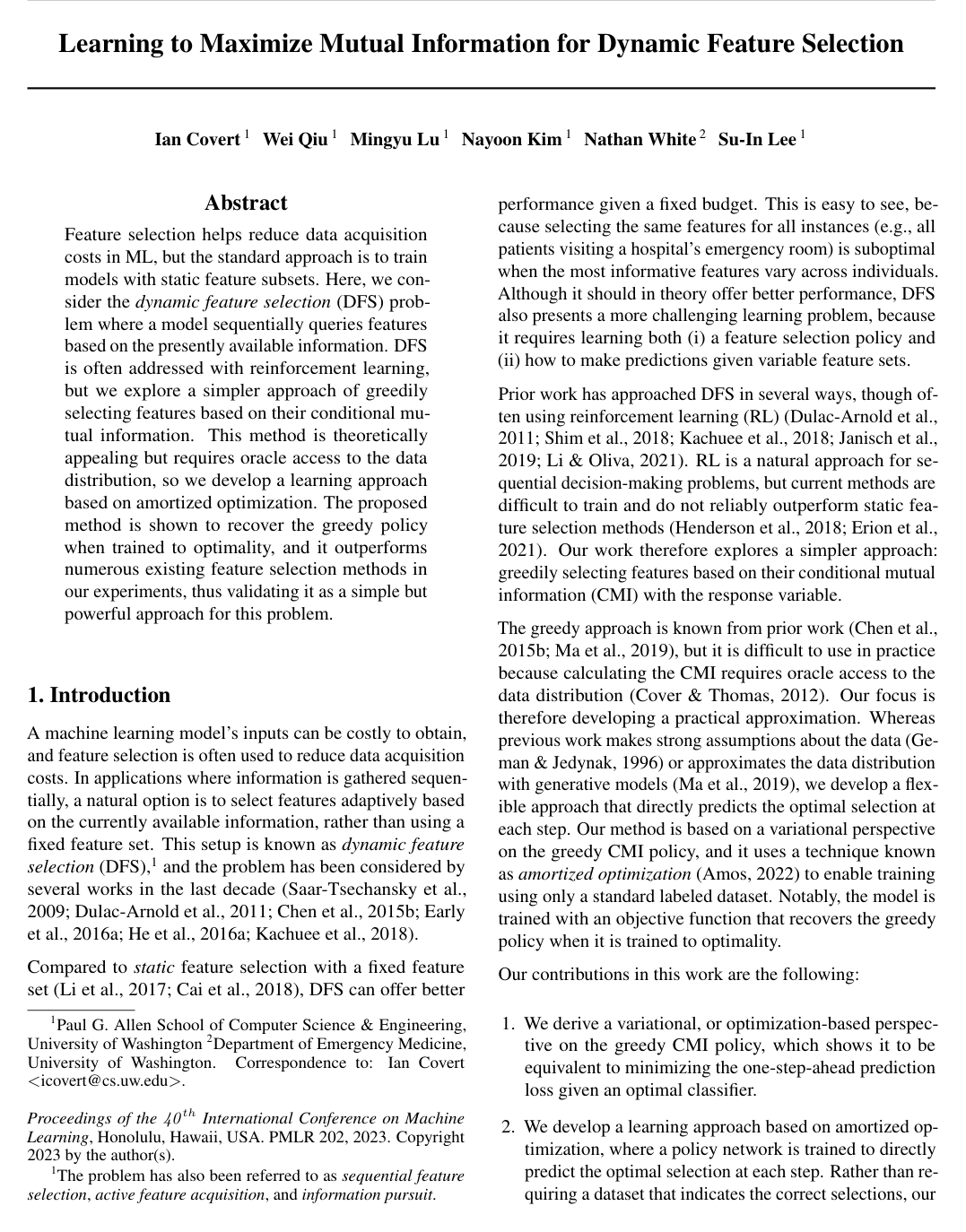
Cover for Learning to Maximize Mutual Information for Dynamic Feature Selection

Abstract

Feature selection helps reduce data acquisition costs in ML, but the standard approach is to train models with static feature subsets. Here, we consider the dynamic feature selection (DFS) problem where a model sequentially queries features based on the presently available information. DFS is often addressed with reinforcement learning, but we explore a simpler approach of greedily selecting features based on their conditional mutual information. This method is theoretically appealing but requires oracle access to the data distribution, so we develop a learning approach based on amortized optimization. The proposed method is shown to recover the greedy policy when trained to optimality, and it outperforms numerous existing feature selection methods in our experiments, thus validating it as a simple but powerful approach for this problem.

Topics

budgets classification methods classifiers generative model genetic selection image classification inference input features mutual informations optimization

Keywords

dynamic feature selection mutual information information pursuit feature acquisition sequential decision-making reinforcement learning imitation learning feature budget

1. Introduction
2. Problem formulation
2.1. Notation
2.2. Dynamic feature selection
3. Greedy information maximization
3.1. The greedy selection policy
3.2. Estimating conditional mutual information
4. Proposed method
4.1. A variational perspective on CMI
4.2. An amortized optimization approach
4.3. Training with a continuous relaxation
5. Related work
6. Experiments
6.1. Tabular datasets
6.2. Image classification datasets
7. Conclusion
Acknowledgements
References
A. Proofs
B. Datasets
B.1. MiniBooNE and spam classification
B.2. Diabetes classification
B.3. Image classification datasets
B.4. Emergency medicine datasets
C. Baselines
C.1. Global feature importance methods
C.2. Local feature importance methods
C.3. Differentiable feature selection
C.4. CMI estimation
C.5. Opportunistic learning
D. Training approach and hyperparameters
D.1. Training pseudocode
Algorithm 1: Training pseudocode
D.2. Model selection
D.3. Hyperparameters
D.4. Feature grouping
E. Additional results

Knowls

Knowl 1 — Greedy conditional-mutual-information policy
definition
For dynamic feature selection, let $x=(x_1,\ldots,x_d)$ be a random input with $d$ features, let $y$ be the response, and let $s\subseteq[d]$ be the indices already observed. The greedy conditional mutual information (CMI) policy selects the unobserved feature with the greatest information about $y$ conditional on the observed features:

$\pi^*(x_s)=\arg\max_{i\notin s} I(y;x_i\mid x_s),\qquad I(y;x_i\mid x_s)=D_{\mathrm{KL}}\!\left(p(x_i,y\mid x_s)\,\middle\|\,p(x_i\mid x_s)p(y\mid x_s)\right).$

Here $x_s$ denotes the values of the features indexed by $s$ , $p$ is the data distribution, and $D_{\mathrm{KL}}$ is Kullback–Leibler divergence. The rule is applied again after each selection, so the next feature depends on the features already acquired.
Knowl 2 — One-step prediction loss characterizes greedy selection
theoretical result
Suppose feature selection uses only the currently observed features, not the unobserved feature values or the response. For a fixed observed set $s$ , consider the expected prediction loss after querying feature $i\notin s$ and predicting from $x_{s\cup\{i\}}$ . With discrete $y$ and cross-entropy loss, the optimal predictor is the Bayes classifier $p(y\mid x_{s\cup\{i\}})$ , and the expected loss for choosing $i$ is $\mathbb{E}_{X_i\mid X_s}[H(Y\mid X_s,X_i)]$ . Consequently, minimizing this one-step loss is equivalent to maximizing $I(Y;X_i\mid X_s)$ .

For continuous $y$ with squared-error loss, the optimal predictor is $\mathbb{E}[Y\mid X_{s\cup\{i\}}]$ , and the expected one-step loss for choosing $i$ is $\mathbb{E}_{X_i\mid X_s}[\operatorname{Var}(Y\mid X_s,X_i)]$ . Thus, in this setting the corresponding greedy rule selects the feature with the smallest expected conditional variance. These are local, one-step criteria; they do not assert that a greedy sequence is globally optimal for every fixed feature budget.
Knowl 3 — Amortized objective recovers the greedy CMI policy
theoretical result
Let a policy network $\pi(x_s;\phi)$ output a probability distribution over the $d$ feature indices, and let a predictor network $f(x_s;\theta)$ predict the response. Train them using labeled examples by minimizing the expected one-step-ahead loss

$\mathcal{L}(\theta,\phi)=\mathbb{E}_{(X,Y)}\mathbb{E}_{S\sim p(S)}\mathbb{E}_{i\sim\pi(X_S;\phi)}\left[\ell\bigl(f(X_{S\cup\{i\}};\theta),Y\bigr)\right],$

where $S$ is a random feature subset, and $p(S)>0$ for every subset with $|S|<d$ . In classification with discrete $Y$ and cross-entropy loss, if the predictor and policy function classes can represent their optima, a global optimum has $f(X_S;\theta^*)=p(Y\mid X_S)$ and places all policy probability on an index maximizing $I(Y;X_i\mid X_S)$ , when that maximizing index is unique. If several indices tie, an optimal policy may distribute probability among the maximizers. The objective therefore learns the greedy choice directly from a standard labeled dataset, without requiring target labels for the correct feature selections.
Knowl 4 — Concrete-relaxed training procedure
algorithm
The method trains a policy and predictor jointly for a fixed selection budget $k$ . A mask $m\in\{0,1\}^d$ records the features already selected; the networks receive the masked input $x\odot m$ and may also receive the mask to distinguish an unobserved feature from a feature whose value is zero. The policy's logits are relaxed to a differentiable Concrete sample for computing each step's prediction loss, while a discrete one-hot choice updates the mask for the next step. Gradients are not propagated through the sequence of discrete mask updates.
Input: Labeled-data distribution p(x, y), budget k, learning rate γ, positive Concrete temperature τ
Output: Predictor f(x; θ), selection policy π(x; ϕ)
Initialize predictor parameters θ and policy parameters ϕ
while training has not converged do
    Sample a labeled example (x, y)
    Set loss L = 0 and mask m = [0, ..., 0]
    for j = 1 to k do
        Compute policy logits α = π(x ⊙ m; ϕ)
        Sample independent standard Gumbel noise G_i for each feature i
        Set relaxed mask m_soft = max(m, softmax(G + α, τ))
        Set next discrete mask m = max(m, softmax(G + α, 0))
        Add ℓ(f(x ⊙ m_soft; θ), y) to L
    end
    Update θ and ϕ by gradient descent on L with learning rate γ
end
Return f and π
The zero-temperature softmax denotes the one-hot choice; the maximum with the existing mask preserves previously selected features. In practice, training uses a sequence of temperatures, with validation-based early stopping at each temperature. Model selection uses validation loss at temperature zero, which represents discrete selection at inference. The paper does not specify a universal numerical temperature schedule or learning rate. For grouped features, the policy outputs one logit per group and the group mask is projected to the original feature coordinates before masking the input.
Knowl 5 — Fixed-budget dynamic feature-selection objective
definition
In the studied dynamic feature selection setting, an instance begins with no observed features and acquires one feature at a time, with a fixed budget of $k<d$ and uniform feature costs. A policy $\pi$ chooses the next index using only the features currently observed; a predictor $f$ makes a prediction from the acquired values. For response $Y$ , input $X$ , and prediction loss $\ell$ , the quality of the policy–predictor pair is its expected loss after $k$ selections:

$v_k(\pi,f)=\mathbb{E}_{(X,Y)}\left[\ell\bigl(f(X_{S_k}),Y\bigr)\right],$

where $S_k$ is the set of the $k$ indices chosen sequentially by $\pi$ , starting from $S_0=\varnothing$ . The objective is to minimize $v_k(\pi,f)$ . This formulation evaluates the final prediction under a fixed budget, while the proposed learning objective trains choices through their one-step-ahead prediction losses.
Knowl 6 — Tabular results across six datasets
data/table
The table compares static feature-ranking or selection baselines, two CMI-estimation variants, a reinforcement-learning method, and the proposed greedy policy. Entries are mean AUROC, reported on a 0–100 scale, averaged over budgets of 1–10 features; the accompanying intervals are the reported 95% confidence intervals. Results are averaged over five runs. The proposed policy has the highest reported mean on each of the six datasets, including the three emergency-medicine tasks.
Could not parse LaTeX table
The comparison shows that being dynamic alone did not ensure strong performance: Opportunistic Learning and CMI estimation were not consistently competitive with static methods. The proposed learned greedy policy was the strongest of the listed methods on all six tabular datasets under this averaged-budget measure.
Knowl 7 — Image-classification performance with pixels and patches
empirical result
The image experiments evaluate sequential acquisition from partially revealed inputs using top-1 accuracy. On MNIST, individual pixels are features ( $d=784$ ), and fully connected policy and predictor networks are used. The proposed policy reaches nearly 90% accuracy with 10 selected pixels, which the paper reports as roughly 10% higher than the best baseline; it has a substantial advantage over the tested baselines at small budgets. The CMI-estimation baseline is omitted on MNIST because scoring many candidate features is computationally costly.

On CIFAR-10, each $32\times32$ image is divided into $64$ patches of size $4\times4$ . The policy and predictor share a ResNet backbone but have separate output heads. The proposed method is slightly less accurate than the comparison methods at very small patch budgets, but achieves higher accuracy when selecting 6–20 patches. Comparisons use the Concrete Autoencoder, center crops, and random masks; other baselines were omitted for computational cost. CIFAR-10 intervals are 95% confidence intervals across five trials.
Knowl 8 — Training-subset distribution matters
empirical result
The proposed training procedure forms observed feature subsets using selections from the current policy, rather than drawing arbitrary feature subsets. Because each observed subset's one-step optimization is treated independently and gradients are not propagated through successive discrete selections, changing how subsets are sampled changes their training weights without changing the stated global optimum. An MNIST ablation nevertheless shows a substantial empirical effect: training on random subsets performs worse than training on policy-generated subsets at every reported feature budget.
Could not parse LaTeX table
The entries are the reported MNIST accuracies. The gap is already present at 5 selected pixels and remains at 50, supporting the use of policy-relevant subsets during training.
Knowl 9 — Scope and stated limitations
limitation
The formulation and experiments study fixed feature budgets with uniform acquisition costs; they do not handle non-uniform costs or choose a separate ideal budget for each instance. The theoretical result for classification characterizes the global optimum of the one-step amortized objective under adequate function-class expressivity and subset sampling with support over every subset of size less than $d$ ; deterministic selection additionally assumes a unique best feature, while ties permit probability to be shared among maximizers. The paper does not establish that the greedy policy is globally optimal for the full fixed-budget trajectory in general. It identifies extensions to variable budgets, non-uniform costs, and architectures suited to partial structured inputs as directions for further work.

Coverage note — The paper's sampled-prediction CMI estimator is an existing approximation discussed for comparison, not the central new method; detailed baseline implementations and per-feature selection-frequency plots are omitted because they do not add a separate load-bearing contribution beyond the included method and comparative results.

References

1.National health and nutrition examination survey, 2018. URL https://www.cdc.gov/nchs/nhanes.
2.Amos, B. Tutorial on amortized optimization for learning to optimize over continuous domains. arXiv preprint arXiv:2202.00665, 2022.
3.Balın, M. F., Abid, A., and Zou, J. Concrete autoencoders: Differentiable feature selection and reconstruction. In International Conference on Machine Learning, pp. 444–453. PMLR, 2019.
4.Breiman, L. Random forests. Machine Learning, 45(1):5–32, 2001.
5.Cai, J., Luo, J., Wang, S., and Yang, S. Feature selection in machine learning: A new perspective. Neurocomputing, 300:70–79, 2018.
6.Chang, C.-H., Rampasek, L., and Goldenberg, A. Dropout feature ranking for deep learning models. arXiv preprint arXiv:1712.08645, 2017.
7.Chattopadhyay, A., Slocum, S., Haeffele, B. D., Vidal, R., and Geman, D. Interpretable by design: Learning predictors by composing interpretable queries. IEEE Transactions on Pattern Analysis and Machine Intelligence, 2022.
8.Chattopadhyay, A., Chan, K. H. R., Haeffele, B. D., Geman, D., and Vidal, R. Variational information pursuit for interpretable predictions. arXiv preprint arXiv:2302.02876, 2023.
9.Chen, J., Song, L., Wainwright, M., and Jordan, M. Learning to explain: An information-theoretic perspective on model interpretation. In International Conference on Machine Learning, pp. 883–892. PMLR, 2018.
10.Chen, S., Choi, A., and Darwiche, A. Value of information based on decision robustness. In Proceedings of the AAAI Conference on Artificial Intelligence, volume 29, 2015a.
11.Chen, Y., Hassani, S. H., Karbasi, A., and Krause, A. Sequential information maximization: When is greedy near-optimal? In Conference on Learning Theory, pp. 338–363. PMLR, 2015b.
12.Cover, T. and Thomas, J. Elements of Information Theory. Wiley, 2012. ISBN 9781118585771.
13.Covert, I., Lundberg, S. M., and Lee, S.-I. Understanding global feature contributions with additive importance measures. Advances in Neural Information Processing Systems, 33:17212–17223, 2020.
14.Covert, I., Lundberg, S. M., and Lee, S.-I. Explaining by removing: A unified framework for model explanation. Journal of Machine Learning Research, 22:209–1, 2021.
15.Covert, I., Gala, R., Wang, T., Svoboda, K., Lee, S.-I., et al. Predictive and robust gene selection for spatial transcriptomics. bioRxiv, 2022.
16.Das, A. and Kempe, D. Submodular meets spectral: Greedy algorithms for subset selection, sparse approximation and dictionary selection. arXiv preprint arXiv:1102.3975, 2011.
17.Dua, D. and Graff, C. UCI machine learning repository, 2017. URL http://archive.ics.uci.edu/ml.
18.Dulac-Arnold, G., Denoyer, L., Preux, P., and Gallinari, P. Datum-wise classification: a sequential approach to sparsity. In Joint European Conference on Machine Learning and Knowledge Discovery in Databases, pp. 375–390. Springer, 2011.
19.Early, K., Fienberg, S. E., and Mankoff, J. Test time feature ordering with FOCUS: Interactive predictions with minimal user burden. In Proceedings of the 2016 ACM International Joint Conference on Pervasive and Ubiquitous Computing, pp. 992–1003, 2016a.
20.Early, K., Mankoff, J., and Fienberg, S. E. Dynamic question ordering in online surveys. arXiv preprint arXiv:1607.04209, 2016b.
21.Elenberg, E. R., Khanna, R., Dimakis, A. G., and Negahban, S. Restricted strong convexity implies weak submodularity. The Annals of Statistics, 46(6B):3539–3568, 2018.
22.Erion, G., Janizek, J. D., Hudelson, C., Utarnachitt, R. B., McCoy, A. M., Sayre, M. R., White, N. J., and Lee, S.-I. CoAI: Cost-aware artificial intelligence for health care. medRxiv, 2021.
23.Feng, J. and Simon, N. Sparse-input neural networks for high-dimensional nonparametric regression and classification. arXiv preprint arXiv:1711.07592, 2017.
24.Gal, Y. and Ghahramani, Z. Dropout as a bayesian approximation: Representing model uncertainty in deep learning. In International Conference on Machine Learning, pp. 1050–1059. PMLR, 2016.
25.Geman, D. and Jedynak, B. An active testing model for tracking roads in satellite images. IEEE Transactions on Pattern Analysis and Machine Intelligence, 18(1):1–14, 1996.
26.Golovin, D. and Krause, A. Adaptive submodularity: Theory and applications in active learning and stochastic optimization. Journal of Artificial Intelligence Research, 42:427–486, 2011.
27.Grathwohl, W., Choi, D., Wu, Y., Roeder, G., and Duvenaud, D. Backpropagation through the void: Optimizing control variates for black-box gradient estimation. In International Conference on Learning Representations, 2018.
28.Guyon, I. and Elisseeff, A. An introduction to variable and feature selection. Journal of Machine Learning Research, 3(Mar):1157–1182, 2003.
29.He, H., Daumé III, H., and Eisner, J. Cost-sensitive dynamic feature selection. In ICML Inferning Workshop, 2012.
30.He, H., Mineiro, P., and Karampatziakis, N. Active information acquisition. arXiv preprint arXiv:1602.02181, 2016a.
31.He, K., Zhang, X., Ren, S., and Sun, J. Deep residual learning for image recognition. In Proceedings of the IEEE Conference on Computer Vision and Pattern Recognition, pp. 770–778, 2016b.
32.Henderson, P., Islam, R., Bachman, P., Pineau, J., Precup, D., and Meger, D. Deep reinforcement learning that matters. In Proceedings of the AAAI Conference on Artificial Intelligence, volume 32, 2018.
33.Jang, E., Gu, S., and Poole, B. Categorical reparameterization with Gumbel-softmax. arXiv preprint arXiv:1611.01144, 2016.
34.Janisch, J., Pevný, T., and Lisý, V. Classification with costly features using deep reinforcement learning. In Proceedings of the AAAI Conference on Artificial Intelligence, volume 33, pp. 3959–3966, 2019.
35.Jethani, N., Sudarshan, M., Aphinyanaphongs, Y., and Ranganath, R. Have we learned to explain?: How interpretability methods can learn to encode predictions in their interpretations. In International Conference on Artificial Intelligence and Statistics, pp. 1459–1467. PMLR, 2021.
36.Kachuee, M., Goldstein, O., Kärkkäinen, K., Darabi, S., and Sarrafzadeh, M. Opportunistic learning: Budgeted cost-sensitive learning from data streams. In International Conference on Learning Representations, 2018.
37.Kachuee, M., Karkkainen, K., Goldstein, O., Zamanzadeh, D., and Sarrafzadeh, M. Cost-sensitive diagnosis and learning leveraging public health data. arXiv preprint arXiv:1902.07102, 2019.
38.Karayev, S., Baumgartner, T., Fritz, M., and Darrell, T. Timely object recognition. Advances in Neural Information Processing Systems, 25, 2012.
39.Kingma, D. P., Salimans, T., and Welling, M. Variational dropout and the local reparameterization trick. Advances in Neural Information Processing Systems, 28, 2015.
40.Kokhlikyan, N., Miglani, V., Martin, M., Wang, E., Alsallakh, B., Reynolds, J., Melnikov, A., Kliushkina, N., Araya, C., Yan, S., et al. Captum: A unified and generic model interpretability library for PyTorch. arXiv preprint arXiv:2009.07896, 2020.
41.Krizhevsky, A., Hinton, G., et al. Learning multiple layers of features from tiny images. 2009.
42.LeCun, Y., Bottou, L., Bengio, Y., and Haffner, P. Gradient-based learning applied to document recognition. Proceedings of the IEEE, 86(11):2278–2324, 1998.
43.Lee, C., Imrie, F., and van der Schaar, M. Self-supervision enhanced feature selection with correlated gates. In International Conference on Learning Representations, 2021.
44.Lemhadri, I., Ruan, F., and Tibshirani, R. Lassonet: Neural networks with feature sparsity. In International Conference on Artificial Intelligence and Statistics, pp. 10–18. PMLR, 2021.
45.Li, J., Cheng, K., Wang, S., Morstatter, F., Trevino, R. P., Tang, J., and Liu, H. Feature selection: A data perspective. ACM Computing Surveys (CSUR), 50(6):1–45, 2017.
46.Li, Y. and Oliva, J. Active feature acquisition with generative surrogate models. In International Conference on Machine Learning, pp. 6450–6459. PMLR, 2021.
47.Ma, C., Tschiatschek, S., Palla, K., Hernandez-Lobato, J. M., Nowozin, S., and Zhang, C. EDDI: Efficient dynamic discovery of high-value information with partial VAE. In International Conference on Machine Learning, pp. 4234–4243. PMLR, 2019.
48.Ma, C., Tschiatschek, S., Turner, R., Hernandez-Lobato, J. M., and Zhang, C. VAEM: a deep generative model for heterogeneous mixed type data. Advances in Neural Information Processing Systems, 33:11237–11247, 2020.
49.Maddison, C. J., Mnih, A., and Teh, Y. W. The Concrete distribution: A continuous relaxation of discrete random variables. arXiv preprint arXiv:1611.00712, 2016.
50.Melville, P., Saar-Tsechansky, M., Provost, F., and Mooney, R. Active feature-value acquisition for classifier induction. In Fourth IEEE International Conference on Data Mining (ICDM’04), pp. 483–486. IEEE, 2004.
51.Miller, H. W. Plan and operation of the health and nutrition examination survey, United States, 1971-1973. DHEW publication no. (PHS)-Dept. of Health, Education, and Welfare (USA), 1973.
52.Mnih, V., Heess, N., Graves, A., et al. Recurrent models of visual attention. Advances in Neural Information Processing Systems, 27, 2014.
53.Mosesson, M. W. Fibrinogen and fibrin structure and functions. Journal of Thrombosis and Haemostasis, 3(8):1894–1904, 2005.
54.Nazabal, A., Olmos, P. M., Ghahramani, Z., and Valera, I. Handling incomplete heterogeneous data using VAEs. Pattern Recognition, 107:107501, 2020.
55.Paszke, A., Gross, S., Chintala, S., Chanan, G., Yang, E., DeVito, Z., Lin, Z., Desmaison, A., Antiga, L., and Lerer, A. Automatic differentiation in PyTorch. 2017.
56.Randløv, J. and Alstrøm, P. Learning to drive a bicycle using reinforcement learning and shaping. In ICML, volume 98, pp. 463–471. Citeseer, 1998.
57.Roe, B., Yand, H., Zhu, J., Lui, Y., Stancu, I., et al. Boosted decision trees, an alternative to artificial neural networks. Nucl. Instrm. Meth. A, 543:577–584, 2005.
58.Saar-Tsechansky, M., Melville, P., and Provost, F. Active feature-value acquisition. Management Science, 55(4):664–684, 2009.
59.Shim, H., Hwang, S. J., and Yang, E. Joint active feature acquisition and classification with variable-size set encoding. Advances in Neural Information Processing Systems, 31, 2018.
60.Shrikumar, A., Greenside, P., and Kundaje, A. Learning important features through propagating activation differences. In International Conference on Machine Learning, pp. 3145–3153. PMLR, 2017.
61.Srivastava, N., Hinton, G., Krizhevsky, A., Sutskever, I., and Salakhutdinov, R. Dropout: a simple way to prevent neural networks from overfitting. The Journal of Machine Learning Research, 15(1):1929–1958, 2014.
62.Subcommittee, A., Group, I. A. W., et al. Advanced trauma life support (ATLS®): the ninth edition. The Journal of Trauma and Acute Care Surgery, 74(5):1363–1366, 2013.
63.Sundararajan, M., Taly, A., and Yan, Q. Axiomatic attribution for deep networks. In International Conference on Machine Learning, pp. 3319–3328. PMLR, 2017.
64.Sutton, R. S., Barto, A. G., et al. Introduction to reinforcement learning. 1998.
65.Tank, A., Covert, I., Foti, N., Shojaie, A., and Fox, E. B. Neural Granger causality. IEEE Transactions on Pattern Analysis and Machine Intelligence, 44(8):4267–4279, 2021.
66.Tucker, G., Mnih, A., Maddison, C. J., Lawson, J., and Sohl-Dickstein, J. Rebar: Low-variance, unbiased gradient estimates for discrete latent variable models. Advances in Neural Information Processing Systems, 30, 2017.
67.Williams, R. J. Simple statistical gradient-following algorithms for connectionist reinforcement learning. Machine Learning, 8(3):229–256, 1992.
68.Yamada, Y., Lindenbaum, O., Negahban, S., and Kluger, Y. Feature selection using stochastic gates. In International Conference on Machine Learning. PMLR, 2020.
69.Yoon, J., Jordon, J., and van der Schaar, M. INVASE: Instance-wise variable selection using neural networks. In International Conference on Learning Representations, 2018.

Citation

MLA

Covert, I. C., et al. “Learning to Maximize Mutual Information for Dynamic Feature Selection”. International Conference on Machine Learning, vol. 202, 2023, pp. 6424–47, https://proceedings.mlr.press/v202/covert23a.html.

APA

Covert, I. C., Qiu, W., Lu, M., Kim, N. Y., White, N. J., & Lee, S.-I. (2023). Learning to Maximize Mutual Information for Dynamic Feature Selection. International Conference on Machine Learning, 202, 6424–6447. https://proceedings.mlr.press/v202/covert23a.html

Chicago

Covert, I. C., W. Qiu, M. Lu, N. Y. Kim, N. J. White, and S.-I. Lee. 2023. “Learning to Maximize Mutual Information for Dynamic Feature Selection”. International Conference on Machine Learning 202: 6424–47. https://proceedings.mlr.press/v202/covert23a.html.

Harvard

Covert, I.C. et al. (2023) “Learning to Maximize Mutual Information for Dynamic Feature Selection”, International Conference on Machine Learning. PMLR, pp. 6424–6447. Available at: https://proceedings.mlr.press/v202/covert23a.html.

Vancouver

1. Covert IC, Qiu W, Lu M, Kim NY, White NJ, Lee S-I (2023) Learning to Maximize Mutual Information for Dynamic Feature Selection. In: International Conference on Machine Learning. PMLR, pp 6424–6447

BibTeX

@InProceedings{pmlr-v202-covert23a,
  title = 	 {Learning to Maximize Mutual Information for Dynamic Feature Selection},
  author =       {Covert, Ian Connick and Qiu, Wei and Lu, Mingyu and Kim, Na Yoon and White, Nathan J and Lee, Su-In},
  booktitle = 	 {Proceedings of the 40th International Conference on Machine Learning},
  pages = 	 {6424--6447},
  year = 	 {2023},
  editor = 	 {Krause, Andreas and Brunskill, Emma and Cho, Kyunghyun and Engelhardt, Barbara and Sabato, Sivan and Scarlett, Jonathan},
  volume = 	 {202},
  series = 	 {Proceedings of Machine Learning Research},
  month = 	 {23--29 Jul},
  publisher =    {PMLR},
  pdf = 	 {https://proceedings.mlr.press/v202/covert23a/covert23a.pdf},
  url = 	 {https://proceedings.mlr.press/v202/covert23a.html},
  abstract = 	 {Feature selection helps reduce data acquisition costs in ML, but the standard approach is to train models with static feature subsets. Here, we consider the dynamic feature selection (DFS) problem where a model sequentially queries features based on the presently available information. DFS is often addressed with reinforcement learning, but we explore a simpler approach of greedily selecting features based on their conditional mutual information. This method is theoretically appealing but requires oracle access to the data distribution, so we develop a learning approach based on amortized optimization. The proposed method is shown to recover the greedy policy when trained to optimality, and it outperforms numerous existing feature selection methods in our experiments, thus validating it as a simple but powerful approach for this problem.}
}

Metadata:DOI registry

Access the Paper

This paper is available from its original source. Click below to access the PDF.

Open PDF

License: https://creativecommons.org/licenses/by/4.0/

Learning to Maximize Mutual Information for Dynamic Feature Selection

Abstract

Topics

Keywords

Table of Contents

Knowls

Knowl 1 — Greedy conditional-mutual-information policy

Knowl 2 — One-step prediction loss characterizes greedy selection

Knowl 3 — Amortized objective recovers the greedy CMI policy

Knowl 4 — Concrete-relaxed training procedure

Knowl 5 — Fixed-budget dynamic feature-selection objective

Knowl 6 — Tabular results across six datasets

Knowl 7 — Image-classification performance with pixels and patches

Knowl 8 — Training-subset distribution matters

Knowl 9 — Scope and stated limitations

References

Citation

BibTeX

Access the Paper