Large Margin Methods for Structured and Interdependent Output Variables

Ioannis Tsochantaridis
[email protected]
Google, Inc.
Mountain View, CA 94043, USA

Thorsten Joachims
[email protected]
Department of Computer Science
Cornell University
Ithaca, NY 14853, USA

Thomas Hofmann
[email protected]
Darmstadt University of Technology
Fraunhofer IPSI
Darmstadt, Germany

Yasemin Altun
[email protected]
Toyota Technological Institute
Chicago, IL 60637, USA

Editor: Yoram Singer

Abstract

Learning general functional dependencies between arbitrary input and output spaces is one of the key challenges in computational intelligence. While recent progress in machine learning has mainly focused on designing flexible and powerful input representations, this paper addresses the complementary issue of designing classification algorithms that can deal with more complex outputs, such as trees, sequences, or sets. More generally, we consider problems involving multiple dependent output variables, structured output spaces, and classification problems with class attributes. In order to accomplish this, we propose to appropriately generalize the well-known notion of a separation margin and derive a corresponding maximum-margin formulation. While this leads to a quadratic program with a potentially prohibitive, i.e. exponential, number of constraints, we present a cutting plane algorithm that solves the optimization problem in polynomial time for a large class of problems. The proposed method has important applications in areas such as computational biology, natural language processing, information retrieval/extraction, and optical character recognition. Experiments from various domains involving different types of output spaces emphasize the breadth and generality of our approach.

Executive Summary: Many complex modern information systems require making predictions that are structured objects—such as full grammatical parse trees, sequence alignments, or hierarchical classifications—rather than simple binary or single-class labels. Traditional machine learning techniques, such as standard support vector machines, are designed for simple scalar or flat multiclass outputs. Treating each distinct structured output as an independent class is computationally intractable because the number of possible output structures grows exponentially with sequence or problem size.

The article establishes and evaluates a generalized maximum-margin framework capable of learning functional mappings from arbitrary input spaces to complex, interdependent output structures. It also evaluates an efficient cutting-plane optimization algorithm designed to solve the resulting large-margin formulation in polynomial time while accommodating problem-specific loss functions.

The proposed approach uses joint feature mappings over inputs and outputs combined with generalized margin maximization. While this formulation produces an exponential number of margin constraints, the authors prove that a cutting-plane algorithm needs to identify only a small, polynomially bounded working set of active constraints to achieve an accurate approximation within a user-specified tolerance. The framework was evaluated through formal theoretical proofs and empirical experiments spanning four distinct domains: hierarchical patent classification using the WIPO-alpha corpus, named entity recognition on Spanish news text, synthetic biological sequence alignment, and natural language parsing on the Penn Treebank Wall Street Journal dataset.

The findings confirm both the theoretical tractability and empirical superiority of the proposed framework. First, the cutting-plane method converges in polynomial time, adding a number of constraints that scales independently of the total size of the output space and grows sub-linearly with the training sample size. Second, in natural language parsing, tailoring the model directly to the task-specific F1 evaluation metric raised performance to an 88.5% F1 score, significantly outperforming traditional probabilistic context-free grammars at 86.0%. Third, in named entity recognition, the large-margin approach achieved a low 5.08% error rate, outperforming generative hidden Markov models at 9.36%, perceptron models at 5.94%, and conditional random fields at 5.17%. Fourth, in hierarchical patent categorization, exploiting the taxonomy and optimizing for tree-structured loss reduced loss by roughly 12% to 14% compared to standard flat multiclass support vector machines.

These results demonstrate that machine learning systems can directly optimize complex, domain-specific evaluation metrics without being restricted to standard zero-one classification error. This provides improved predictive accuracy, reduced decision risk, and greater modeling flexibility in high-value applications such as computational biology, document routing, and language understanding. Unlike generative probabilistic frameworks that require rigid independence assumptions, this discriminative approach enables the integration of overlapping features and non-linear kernel representations.

Organizations deploying structured prediction models should consider adopting this generalized large-margin architecture, implemented in the publicly available SVMstruct software. Teams should define application-specific loss functions directly aligned with operational objectives, such as custom tree loss for classification taxonomies or overlap measures for information extraction. In practice, setting the precision tolerance parameter to 0.1 strikes an effective balance between optimization speed and final predictive performance.

A primary operational requirement and limitation of this framework is the need for an efficient separation oracle or dynamic programming routine (such as the Viterbi or CKY algorithm) to identify the most violated constraints during training. If the underlying decoding problem cannot be solved efficiently, the exact training algorithm becomes intractable. However, for the wide range of problems where such inference is feasible, confidence in the method's theoretical guarantees and empirical performance remains high.

1. Introduction

Section Summary: This paper addresses the challenge of training models to map input patterns to complex structured outputs such as sequences, trees, or graphs, rather than simple class labels or numeric values. It extends large-margin methods like support vector machines to these settings by using joint feature representations that capture dependencies within the outputs, enabling efficient learning even when the number of possible structures is enormous. The resulting algorithms are positioned as more flexible and accurate than related approaches like perceptron training or ranking methods, with evaluations on tasks including sequence labeling and natural language parsing.

This paper deals with the general problem of learning a mapping from input vectors or patterns $\mathbf{x} \in \mathcal{X}$ to discrete response variables $\mathbf{y} \in \mathcal{Y}$, based on a training sample of input-output pairs $(\mathbf{x}_1, \mathbf{y}_1), \dots, (\mathbf{x}_n, \mathbf{y}_n) \in \mathcal{X} \times \mathcal{Y}$ drawn from some fixed but unknown probability distribution. Unlike multiclass classification, where the output space consists of an arbitrary finite set of labels or class identifiers, $\mathcal{Y} = {1, \dots, K}$, or regression, where $\mathcal{Y} = \mathbb{R}$ and the response variable is a scalar, we consider the case where elements of $\mathcal{Y}$ are structured objects such as sequences, strings, trees, lattices, or graphs. Such problems arise in a variety of applications, ranging from multilabel classification and classification with class taxonomies, to label sequence learning, sequence alignment learning, and supervised grammar learning, to name just a few. More generally, these problems fall into two generic cases: first, problems where classes themselves can be characterized by certain class-specific attributes and learning should occur across classes as much as across patterns; second, problems where $\mathbf{y}$ represents a macro-label, i.e. describes a configuration over components or state variables $\mathbf{y} = (y^1, \dots, y^T)$, with possible dependencies between these state variables.

We approach these problems by generalizing large margin methods, more specifically multiclass support vector machines (SVMs) (Weston and Watkins, 1998; Crammer and Singer, 2001), to the broader problem of learning structured responses. The naive approach of treating each structure as a separate class is often intractable, since it leads to a multiclass problem with a very large number of classes. We overcome this problem by specifying discriminant functions that exploit the structure and dependencies within $\mathcal{Y}$. In that respect our approach follows the work of Collins (2002) on perceptron learning with a similar class of discriminant functions. However, the maximum-margin algorithm we propose has advantages in terms of accuracy and tunability to specific loss functions. A maximum-margin algorithm has also been proposed by Collins and Duffy (2002a) in the context of natural language processing. However, it depends on the size of the output space, therefore it requires some external process to enumerate a small number of candidate outputs $\mathbf{y}$ for a given input $\mathbf{x}$. The same is true also for other ranking algorithms (Cohen et al., 1999; Herbrich et al., 2000; Schapire and Singer, 2000; Crammer and Singer, 2002; Joachims, 2002). In contrast, we have proposed an efficient algorithm (Hofmann et al., 2002; Altun et al., 2003; Joachims, 2003) even in the case of very large output spaces, that takes advantage of the sparseness of the maximum-margin solution.

A different maximum-margin algorithm that can deal with very large output sets, maximum margin Markov networks, has been independently proposed by Taskar et al. (2004a). The structure of the output is modeled by a Markov network, and by employing a probabilistic interpretation of the dual formulation of the problem, Taskar et al. (2004a) propose a reparameterization of the problem, that leads to an efficient algorithm, as well as generalization bounds that do not depend on the size of the output space. The proposed reparameterization, however, assumes that the loss function can be decomposed in the the same fashion as the feature map, thus does not support arbitrary loss functions that may be appropriate for specific applications.

On the surface our approach is related to the kernel dependency estimation approach described in Weston et al. (2003). There, however, separate kernel functions are defined for the input and output space, with the idea to encode a priori knowledge about the similarity or loss function in output space. In particular, this assumes that the loss is input dependent and known beforehand. More specifically, in Weston et al. (2003) a kernel PCA is used in the feature space defined over $\mathbf{y}$ to reduce the problem to a (small) number of independent regression problems. The latter corresponds to an unsupervised embedding (followed by dimension reduction) performed in the output space and no information about the patterns $\mathbf{x}$ is utilized in defining this low-dimensional representation. In contrast, the key idea in our approach is not primarily to define more complex functions, but to deal with more complex output spaces by extracting combined features over inputs and outputs.

For a large class of structured models, we propose a novel SVM algorithm that allows us to learn mappings involving complex structures in polynomial time despite an exponential (or infinite) number of possible output values. In addition to respective theoretical results, we empirically evaluate our approach for a number of specific problem instantiations: classification with class taxonomies, label sequence learning, sequence alignment, and natural language parsing. This paper extends Tsochantaridis et al. (2004) with additional theoretical and empirical results.

The rest of the paper is organized as follows: Section 2 presents the general framework of large margin learning over structured output spaces using representations of input-output pairs via joint feature maps. Section 3 describes and analyzes a generic algorithm for solving the resulting optimization problems. Sections 4 and 5 discuss numerous important special cases and experimental results, respectively.

2. Large Margin Learning with Joint Feature Maps

Section Summary: The section introduces a general framework for learning mappings from inputs like sentences to complex structured outputs like parse trees, by training a linear discriminant function over joint feature representations of input-output pairs and predicting via maximization of this function. This setup supports kernel methods for efficient computation and can represent models like probabilistic context-free grammars, where parse trees are scored by weighted grammar-rule counts. It further addresses the need for custom loss functions that measure partial correctness in structured predictions, along with minimizing the associated risk on training data.

{width=80%}

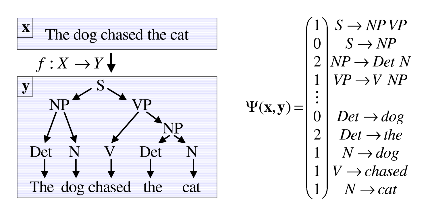
We are interested in the general problem of learning functions $f : \mathcal{X} \to \mathcal{Y}$ between input spaces $\mathcal{X}$ and arbitrary discrete output spaces $\mathcal{Y}$ based on a training sample of input-output pairs. As an illustrating example, which we will continue to use as a prototypical application in the sequel, consider the case of natural language parsing, where the function $f$ maps a given sentence $\mathbf{x}$ to a parse tree $\mathbf{y}$. This is depicted graphically in Figure 1.

The approach we pursue is to learn a discriminant function $F : \mathcal{X} \times \mathcal{Y} \to \mathbb{R}$ over input-output pairs from which we can derive a prediction by maximizing $F$ over the response variable for a specific given input $\mathbf{x}$. Hence, the general form of our hypotheses $f$ is

$ f(\mathbf{x};\mathbf{w}) = \operatorname{argmax}_{\mathbf{y} \in \mathcal{Y}} F(\mathbf{x}, \mathbf{y}; \mathbf{w}),\tag{1} $

where $\mathbf{w}$ denotes a parameter vector. It might be useful to think of $F$ as a compatibility function that measures how compatible pairs $(\mathbf{x}, \mathbf{y})$ are, or, alternatively, $-F$ can be thought of as a $\mathbf{w}$-parameterized family of cost functions, which we try to design in such a way that the minimum of $F(\mathbf{x}, \cdot; \mathbf{w})$ is at the desired output $\mathbf{y}$ for inputs $\mathbf{x}$ of interest.

Throughout this paper, we assume $F$ to be linear in some combined feature representation of inputs and outputs $\Psi(\mathbf{x}, \mathbf{y})$, i.e.

$ F(\mathbf{x}, \mathbf{y}; \mathbf{w}) = \langle \mathbf{w}, \Psi(\mathbf{x}, \mathbf{y}) \rangle.\tag{2} $

The specific form of $\Psi$ depends on the nature of the problem and special cases will be discussed subsequently. However, whenever possible we will develop learning algorithms and theoretical results for the general case. Since we want to exploit the advantages of kernel-based method, we will pay special attention to cases where the inner product in the joint representation can be efficiently computed via a joint kernel function $J((\mathbf{x}, \mathbf{y}), (\mathbf{x}', \mathbf{y}')) = \langle \Psi(\mathbf{x}, \mathbf{y}), \Psi(\mathbf{x}', \mathbf{y}') \rangle$.

Using again natural language parsing as an illustrative example, we can chose $F$ such that we get a model that is isomorphic to a probabilistic context free grammar (PCFG) (cf. Manning and Schuetze, 1999). Each node in a parse tree $\mathbf{y}$ for a sentence $\mathbf{x}$ corresponds to grammar rule $g_j$, which in turn has a score $w_j$. All valid parse trees $\mathbf{y}$ (i.e. trees with a designated start symbol $S$ as the root and the words in the sentence $\mathbf{x}$ as the leaves) for a sentence $\mathbf{x}$ are scored by the sum of the $w_j$ of their nodes. This score can thus be written in the form of Equation (2), with $\Psi(\mathbf{x}, \mathbf{y})$ denoting a histogram vector of counts (how often each grammar rule $g_j$ occurs in the tree $\mathbf{y}$). $f(\mathbf{x}; \mathbf{w})$ can be efficiently computed by finding the structure $\mathbf{y} \in \mathcal{Y}$ that maximizes $F(\mathbf{x}, \mathbf{y}; \mathbf{w})$ via the CKY algorithm (Younger, 1967; Manning and Schuetze, 1999).

2.1 Loss Functions and Risk Minimization

The standard zero-one loss function typically used in classification is not appropriate for most kinds of structured responses. For example, in natural language parsing, a parse tree that is almost correct and differs from the correct parse in only one or a few nodes should be treated differently from a parse tree that is completely different. Typically, the correctness of a predicted parse tree is measured by its $F_1$ score (see e.g. Johnson, 1998), the harmonic mean of precision and recall as calculated based on the overlap of nodes between the trees.

In order to quantify the accuracy of a prediction, we will consider learning with arbitrary loss functions $\Delta : \mathcal{Y} \times \mathcal{Y} \to \mathbb{R}$. Here $\Delta(\mathbf{y}, \hat{\mathbf{y}})$ quantifies the loss associated with a prediction $\hat{\mathbf{y}}$, if the true output value is $\mathbf{y}$. It is usually sufficient to restrict attention to zero diagonal loss functions with $\Delta(\mathbf{y}, \mathbf{y}) = 0$ and for which furthermore $\Delta(\mathbf{y}, \mathbf{y}') > 0$ for $\mathbf{y} \neq \mathbf{y}'$.[^1] Moreover, we assume the loss is bounded for every given target value $\mathbf{y}^*$, i.e. $\max_{\mathbf{y}} {\Delta(\mathbf{y}^*, \mathbf{y})}$ exists.

[^1]: Cases where $\Delta(\mathbf{y}, \mathbf{y}') = 0$ for $\mathbf{y} \neq \mathbf{y}'$ can be dealt with, but lead to additional technical overhead, which we chose to avoid for the sake of clarity.

We investigate a supervised learning scenario, where input-output pairs $(\mathbf{x}, \mathbf{y})$ are generated according to some fixed distribution $P(\mathbf{x}, \mathbf{y})$ and the goal is to find a function $f$ in a given hypothesis class such that the risk,

$ \mathcal{R}^\Delta_P(f) = \int_{\mathcal{X} \times \mathcal{Y}} \Delta(\mathbf{y}, f(\mathbf{x})) dP(\mathbf{x}, \mathbf{y}), $

is minimized. Of course, $P$ is unknown and following the supervised learning paradigm, we assume that a finite training set of pairs $S = {(\mathbf{x}_i, \mathbf{y}_i) \in \mathcal{X} \times \mathcal{Y} : i = 1, \dots, n}$ generated i.i.d. according to $P$ is given. The performance of a function $f$ on the training sample $S$ is described by the empirical risk,

$ \mathcal{R}^\Delta_S(f) = \frac{1}{n} \sum_{i=1}^n \Delta(\mathbf{y}_i, f(\mathbf{x}_i)), $

which is simply the expected loss under the empirical distribution induced by $S$. For $\mathbf{w}$-parameterized hypothesis classes, we will also write $\mathcal{R}^\Delta_P(\mathbf{w}) \equiv \mathcal{R}^\Delta_P(f(\cdot; \mathbf{w}))$ and similarly for the empirical risk.

2.2 Margin Maximization

We consider various scenarios for the generalization of support vector machine learning over structured outputs. We start with the simple case of hard-margin SVMs, followed by soft-margin SVMs, and finally we propose two approaches for the case of loss-sensitive SVMs, which is the most general case and subsumes the former ones.

2.2.1 Separable Case

First, we consider the case where there exists a function $f$ parameterized by $\mathbf{w}$ such that the empirical risk is zero. The condition of zero training error can then be compactly written as a set of nonlinear constraints

$ \forall i \in {1, \dots, n} : \max_{\mathbf{y} \in \mathcal{Y} \setminus \mathbf{y}_i} { \langle \mathbf{w}, \Psi(\mathbf{x}_i, \mathbf{y}) \rangle } \le \langle \mathbf{w}, \Psi(\mathbf{x}_i, \mathbf{y}_i) \rangle .\tag{3} $

Notice that this holds independently of the loss functions, since we have assumed that $\Delta(\mathbf{y}, \mathbf{y}) = 0$ and $\Delta(\mathbf{y}, \mathbf{y}') > 0$ for $\mathbf{y} \neq \mathbf{y}'$.

Every one of the nonlinear inequalities in Equation (3) can be equivalently replaced by $|\mathcal{Y}| - 1$ linear inequalities, resulting in a total of $n|\mathcal{Y}| - n$ linear constraints,

$ \forall i \in {1, \dots, n}, , \forall \mathbf{y} \in \mathcal{Y} \setminus \mathbf{y}_i : \langle \mathbf{w}, \Psi(\mathbf{x}_i, \mathbf{y}_i) - \Psi(\mathbf{x}_i, \mathbf{y}) \rangle \ge 0.\tag{4} $

As we will often encounter terms involving feature vector differences of the type appearing in Equation (4), we define $\delta\Psi_i(\mathbf{y}) \equiv \Psi(\mathbf{x}_i, \mathbf{y}_i) - \Psi(\mathbf{x}_i, \mathbf{y})$ so that the constraints can be more compactly written as $\langle \mathbf{w}, \delta\Psi_i(\mathbf{y}) \rangle \ge 0$.

If the set of inequalities in Equation (4) is feasible, there will typically be more than one solution $\mathbf{w}^*$. To specify a unique solution, we propose to select the $\mathbf{w}$ for which the separation margin $\gamma$, i.e. the minimal differences between the score of the correct label $\mathbf{y}i$ and the closest runner-up $\hat{\mathbf{y}}(\mathbf{w}) = \operatorname{argmax}{\mathbf{y} \neq \mathbf{y}_i} \langle \mathbf{w}, \Psi(\mathbf{x}_i, \mathbf{y}) \rangle$, is maximal. This generalizes the maximum-margin principle employed in support vector machines (Vapnik, 1998) to the more general case considered in this paper. Restricting the $L_2$ norm of $\mathbf{w}$ to make the problem well-posed leads to the following optimization problem:

$ \max_{\gamma, \mathbf{w} : |\mathbf{w}| = 1} \gamma $

$ \text{s.t.} \ \forall i \in {1, \dots, n}, , \forall \mathbf{y} \in \mathcal{Y} \setminus \mathbf{y}_i : \langle \mathbf{w}, \delta\Psi_i(\mathbf{y}) \rangle \ge \gamma . $

This problem can be equivalently expressed as a convex quadratic program in standard form

$ \text{SVM}0 : \quad \min{\mathbf{w}} \frac{1}{2} |\mathbf{w}|^2\tag{5} $

$ \text{s.t.} \ \forall i, , \forall \mathbf{y} \in \mathcal{Y} \setminus \mathbf{y}_i : \langle \mathbf{w}, \delta\Psi_i(\mathbf{y}) \rangle \ge 1.\tag{6} $

2.2.2 Soft-Margin Maximization

To allow errors in the training set, we introduce slack variables and propose to optimize a soft-margin criterion. As in the case of multiclass SVMs, there are at least two ways of introducing slack variables. One may introduce a single slack variable $\xi_i$ for violations of the nonlinear constraints (i.e. every instance $\mathbf{x}_i$) (Crammer and Singer, 2001) or one may penalize margin violations for every linear constraint (i.e. every instance $\mathbf{x}_i$ and output $\mathbf{y} \neq \mathbf{y}_i$) (Weston and Watkins, 1998; Har-Peled et al., 2002). Since the former will result in a (tighter) upper bound on the empirical risk (cf. Proposition 1) and offers some advantages in the proposed optimization scheme (cf. Section 3), we have focused on this formulation. Adding a penalty term that is linear in the slack variables to the objective, results in the quadratic program

$ \text{SVM}1 : \quad \min{\mathbf{w}, \boldsymbol{\xi}} \frac{1}{2} |\mathbf{w}|^2 + \frac{C}{n} \sum_{i=1}^n \xi_i\tag{7} $

$ \text{s.t.} \ \forall i, , \forall \mathbf{y} \in \mathcal{Y} \setminus \mathbf{y}_i : \langle \mathbf{w}, \delta\Psi_i(\mathbf{y}) \rangle \ge 1 - \xi_i, , \xi_i \ge 0. $

Alternatively, we can also penalize margin violations by a quadratic term leading to the following optimization problem:

$ \text{SVM}2 : \quad \min{\mathbf{w}, \boldsymbol{\xi}} \frac{1}{2} |\mathbf{w}|^2 + \frac{C}{2n} \sum_{i=1}^n \xi_i^2 $

$ \text{s.t.} \ \forall i, , \forall \mathbf{y} \in \mathcal{Y} \setminus \mathbf{y}_i : \langle \mathbf{w}, \delta\Psi_i(\mathbf{y}) \rangle \ge 1 - \xi_i. $

In both cases, $C > 0$ is a constant that controls the trade-off between training error minimization and margin maximization.

2.2.3 General Loss Functions: Slack Re-scaling

The first approach we propose for the case of arbitrary loss functions, is to re-scale the slack variables according to the loss incurred in each of the linear constraints. Intuitively, violating a margin constraint involving a $\mathbf{y} \neq \mathbf{y}_i$ with high loss $\Delta(\mathbf{y}_i, \mathbf{y})$ should be penalized more severely than a violation involving an output value with smaller loss. This can be accomplished by multiplying the margin violation by the loss, or equivalently, by scaling the slack variable with the inverse loss, which yields

$ \text{SVM}1^{\Delta s} : \quad \min{\mathbf{w}, \boldsymbol{\xi}} \frac{1}{2} |\mathbf{w}|^2 + \frac{C}{n} \sum_{i=1}^n \xi_i $

$ \text{s.t.} \ \forall i, , \forall \mathbf{y} \in \mathcal{Y} \setminus \mathbf{y}_i : \langle \mathbf{w}, \delta\Psi_i(\mathbf{y}) \rangle \ge 1 - \frac{\xi_i}{\Delta(\mathbf{y}_i, \mathbf{y})}. $

A justification for this formulation is given by the subsequent proposition.

Proposition 1 Denote by $\boldsymbol{\xi}^(\mathbf{w})$ the optimal solution of the slack variables in $\text{SVM}1^{\Delta s}$ for a given weight vector $\mathbf{w}$. Then $\frac{1}{n} \sum{i=1}^n \xi_i^*$ is an upper bound on the empirical risk $\mathcal{R}^\Delta_S(\mathbf{w})$.*

Proof Notice first that $\xi_i^* = \max { 0, \max_{\mathbf{y} \neq \mathbf{y}_i} { \Delta(\mathbf{y}_i, \mathbf{y}) (1 - \langle \mathbf{w}, \delta\Psi_i(\mathbf{y}) \rangle) } }$.
Case 1: If $f(\mathbf{x}_i; \mathbf{w}) = \mathbf{y}_i$, then $\xi_i^* \ge 0 = \Delta(\mathbf{y}_i, f(\mathbf{x}_i; \mathbf{w}))$ and the loss is trivially upper bounded.
Case 2: If $\hat{\mathbf{y}} \equiv f(\mathbf{x}_i; \mathbf{w}) \neq \mathbf{y}_i$, then $\langle \mathbf{w}, \delta\Psi_i(\hat{\mathbf{y}}) \rangle \le 0$ and thus $\frac{\xi_i^*}{\Delta(\mathbf{y}_i, \hat{\mathbf{y}})} \ge 1$ which is equivalent to $\xi_i^* \ge \Delta(\mathbf{y}_i, \hat{\mathbf{y}})$.
Since the bound holds for every training instance, it also holds for the average.

The optimization problem $\text{SVM}_2^{\Delta s}$ can be derived analogously, where $\Delta(\mathbf{y}_i, \mathbf{y})$ is replaced by $\sqrt{\Delta(\mathbf{y}_i, \mathbf{y})}$ in order to obtain an upper bound on the empirical risk.

2.2.4 General Loss Functions: Margin Re-scaling

In addition to this slack re-scaling approach, a second way to include loss functions is to re-scale the margin as proposed by Taskar et al. (2004a) for the special case of the Hamming loss. It is straightforward to generalize this method to general loss functions. The margin constraints in this setting take the following form:

$ \forall i, , \forall \mathbf{y} \in \mathcal{Y} : \langle \mathbf{w}, \delta\Psi_i(\mathbf{y}) \rangle \ge \Delta(\mathbf{y}_i, \mathbf{y}) - \xi_i.\tag{8} $

The set of constraints in Equation (8) combined with the objective in Equation (7) yield an optimization problem $\text{SVM}_1^{\Delta m}$ which also results in an upper bound on $\mathcal{R}^\Delta_S(\mathbf{w}^*)$.

Proposition 2 Denote by $\boldsymbol{\xi}^(\mathbf{w})$ the optimal solution of the slack variables in $\text{SVM}1^{\Delta m}$ for a given weight vector $\mathbf{w}$. Then $\frac{1}{n} \sum{i=1}^n \xi_i^*$ is an upper bound on the empirical risk $\mathcal{R}^\Delta_S(\mathbf{w})$.*

Proof The essential observation is that $\xi_i^* = \max { 0, \max_{\mathbf{y}} { \Delta(\mathbf{y}_i, \mathbf{y}) - \langle \mathbf{w}, \delta\Psi_i(\mathbf{y}) \rangle } }$ which is guaranteed to upper bound $\Delta(\mathbf{y}_i, \mathbf{y})$ for $\mathbf{y}$ such that $\langle \mathbf{w}, \delta\Psi_i(\mathbf{y}) \rangle \le 0$.

The optimization problem $\text{SVM}_2^{\Delta m}$ can be derived analogously, where $\Delta(\mathbf{y}_i, \mathbf{y})$ is replaced by $\sqrt{\Delta(\mathbf{y}_i, \mathbf{y})}$.

2.2.5 General Loss Functions: Discussion

Let us discuss some of the advantages and disadvantages of the two formulations presented. An appealing property of the slack re-scaling approach is its scaling invariance.

Proposition 3 Suppose $\Delta' \equiv \eta \Delta$ with $\eta > 0$, i.e. $\Delta'$ is a scaled version of the original loss $\Delta$. Then by re-scaling $C' = C / \eta$, the optimization problems $\text{SVM}_1^{\Delta s}(C)$ and $\text{SVM}_1^{\Delta' s}(C')$ are equivalent as far as $\mathbf{w}$ is concerned. In particular the optimal weight vector $\mathbf{w}^$ is the same in both cases.*

Proof First note that each $\mathbf{w}$ is feasible for $\text{SVM}_1^{\Delta s}$ and $\text{SVM}_1^{\Delta' s}$ in the sense that we can find slack variables such that all the constraints are satisfied. In fact we can chose them optimally and define $H(\mathbf{w}) \equiv \frac{1}{2} |\mathbf{w}|^2 + \frac{C}{n} \sum_i \xi_i^*(\mathbf{w})$ and $H'(\mathbf{w}) \equiv \frac{1}{2} |\mathbf{w}|^2 + \frac{C'}{n} \sum_i \xi_i^{\prime}(\mathbf{w})$, where $\boldsymbol{\xi}^$ and $\boldsymbol{\xi}^{*\prime}$ refer to the optimal slacks in $\text{SVM}_1^{\Delta s}$ and $\text{SVM}_1^{\Delta' s}$, respectively, for given $\mathbf{w}$. It is easy to see that they are given by

$ \xi_i^* = \max { 0, \max_{\mathbf{y} \neq \mathbf{y}_i} { \Delta(\mathbf{y}_i, \mathbf{y}) (1 - \langle \mathbf{w}, \delta\Psi_i(\mathbf{y}) \rangle) } } $

and

$ \xi_i^{*\prime} = \max { 0, \max_{\mathbf{y} \neq \mathbf{y}_i} { \eta \Delta(\mathbf{y}_i, \mathbf{y}) (1 - \langle \mathbf{w}, \delta\Psi_i(\mathbf{y}) \rangle) } }, $

respectively. Pulling $\eta$ out of the max, one gets that $\xi_i^{\prime} = \eta \xi_i^$ and thus $\sum_i \xi_i^* = C \eta \sum_i \xi_i^{\prime} = C' \sum_i \xi_i^{\prime}$. From that it follows immediately that $H = H'$.

In contrast, the margin re-scaling formulation is not invariant under scaling of the loss function. One needs, for example, to re-scale the feature map $\Psi$ by a corresponding scale factor as well. This seems to indicate that one has to calibrate the scaling of the loss and the scaling of the feature map more carefully in the $\text{SVM}_1^{\Delta m}$ formulation. The $\text{SVM}_1^{\Delta s}$ formulation on the other hand, represents the loss scale explicitly in terms of the constant $C$.

A second disadvantage of the margin scaling approach is that it potentially gives significant weight to output values $\mathbf{y} \in \mathcal{Y}$ that are not even close to being confusable with the target values $\mathbf{y}_i$, because every increase in the loss increases the required margin. If one interprets $F(\mathbf{x}_i, \mathbf{y}_i; \mathbf{w}) - F(\mathbf{x}_i, \mathbf{y}; \mathbf{w})$ as a log odds ratio of an exponential family model (Smola and Hofmann, 2003), then the margin constraints may be dominated by incorrect values $\mathbf{y}$ that are exponentially less likely than the target value. To be more precise, notice that in the $\text{SVM}_1^{\Delta s}$ formulation, the penalty part only depends on $\mathbf{y}$ for which $\langle \mathbf{w}, \delta\Psi_i(\mathbf{y}) \rangle \le 1$. These are output values $\mathbf{y}$ that all receive a relatively “high” (i.e. 1-close to the optimum) value of $F(\mathbf{x}, \mathbf{y}; \mathbf{w})$. However, in $\text{SVM}_1^{\Delta m}$, $\xi_i^*$ has to majorize $\Delta(\mathbf{y}i, \mathbf{y}) - \langle \mathbf{w}, \delta\Psi_i(\mathbf{y}) \rangle$ for all $\mathbf{y}$. This means $\xi_i^*$ can be dominated by a value $\hat{\mathbf{y}} = \operatorname{argmax}{\mathbf{y}} { \Delta(\mathbf{y}_i, \mathbf{y}) - \langle \mathbf{w}, \delta\Psi_i(\mathbf{y}) \rangle }$ which has a large loss, but whose value of $F(\mathbf{x}, \mathbf{y}; \mathbf{w})$ comes nowhere near the optimal value of $F$.

3. Support Vector Algorithm for Structured Output Spaces

Section Summary: The section addresses the challenge of solving enormous quadratic optimization problems for structured-output SVMs, where the number of margin constraints grows exponentially with the size of the output space and defeats conventional solvers. It derives the dual quadratic programs for the various separable and non-separable formulations, showing how slack or margin rescaling and linear versus quadratic penalties translate into extra linear constraints or simple modifications of the kernel. The authors then outline a cutting-plane algorithm that iteratively adds only the most violated constraints, thereby obtaining arbitrarily accurate solutions in polynomial time for a wide range of output structures and loss functions.

So far we have not discussed how to solve the optimization problems associated with the various formulations $\text{SVM}_0$, $\text{SVM}_1$, $\text{SVM}_2$, $\text{SVM}_1^{\Delta s}$, $\text{SVM}_1^{\Delta m}$, $\text{SVM}_2^{\Delta s}$, and $\text{SVM}_2^{\Delta m}$. The key challenge is that the size of each of these problems can be immense, since we have to deal with $n|\mathcal{Y}| - n$ margin inequalities. In many cases, $|\mathcal{Y}|$ may be extremely large, in particular, if $\mathcal{Y}$ is a product space of some sort (e.g. in grammar learning, label sequence learning, etc.), its cardinality may grow exponentially in the description length of $\mathbf{y}$. This makes standard quadratic programming solvers unsuitable for this type of problem.

In the following, we will propose an algorithm that exploits the special structure of the maximum-margin problem, so that only a much smaller subset of constraints needs to be explicitly examined. We will show that the algorithm can compute arbitrary close approximations to all SVM optimization problems posed in this paper in polynomial time for a large range of structures and loss functions. Since the algorithm operates on the dual program, we will first derive the Wolfe dual for the various soft margin formulations.

3.1 Dual Programs

We will denote by $\alpha_{(i\mathbf{y})}$ the Lagrange multiplier enforcing the margin constraint for label $\mathbf{y} \neq \mathbf{y}_i$ and example $(\mathbf{x}_i, \mathbf{y}_i)$. Using standard Lagragian duality techniques, one arrives at the following dual quadratic program (QP).

Proposition 4 The objective of the dual problem of $\text{SVM}_0$ from Equation (6) is given by

$ \Theta(\boldsymbol{\alpha}) \equiv -\frac{1}{2} \sum_{i, \mathbf{y} \neq \mathbf{y}i} \sum{j, \bar{\mathbf{y}} \neq \mathbf{y}j} \alpha{(i\mathbf{y})} \alpha_{(j\bar{\mathbf{y}})} J_{(i\mathbf{y})(j\bar{\mathbf{y}})} + \sum_{i, \mathbf{y} \neq \mathbf{y}i} \alpha{(i\mathbf{y})}, $

where $J_{(i\mathbf{y})(j\bar{\mathbf{y}})} = \langle \delta\Psi_i(\mathbf{y}), \delta\Psi_j(\bar{\mathbf{y}}) \rangle$. The dual QP can be formulated as

$ \boldsymbol{\alpha}^* = \operatorname{argmax}_{\boldsymbol{\alpha}} \Theta(\boldsymbol{\alpha}), \quad \text{s.t.} \ \boldsymbol{\alpha} \ge 0. $

Proof (sketch) Forming the Lagrangian function and eliminating the primal variables $\mathbf{w}$ by using the optimality condition

$ \mathbf{w}^*(\boldsymbol{\alpha}) = \sum_i \sum_{\mathbf{y} \neq \mathbf{y}i} \alpha{(i\mathbf{y})} \delta\Psi_i(\mathbf{y}) $

directly leads to the above dual program.

Notice that the $J$ function that generates the quadratic from in the dual objective can be computed from inner products involving values of $\Psi$, which is a simple consequence of the linearity of the inner product. $J$ can hence be alternatively computed from a joint kernel function over $\mathcal{X} \times \mathcal{Y}$.

In the non-separable case, linear penalties introduce additional constraints, whereas the squared penalties modify the kernel function.

Proposition 5 The dual problem to $\text{SVM}_1$ is given by the program in Proposition 4 with additional constraints

$ \sum_{\mathbf{y} \neq \mathbf{y}i} \alpha{(i\mathbf{y})} \le \frac{C}{n}, \quad \forall i = 1, \dots, n. $

In the following, we denote with $\delta(a, b)$ the function that returns 1 if $a = b$, and 0 otherwise.

Proposition 6 The dual problem to $\text{SVM}_2$ is given by the program in Proposition 4 with modified kernel function

$ J_{(i\mathbf{y})(j\bar{\mathbf{y}})} \equiv \langle \delta\Psi_i(\mathbf{y}), \delta\Psi_j(\bar{\mathbf{y}}) \rangle + \delta(i, j) \frac{n}{C}. $

In the non-separable case with slack re-scaling, the loss function is introduced in the constraints for linear penalties and in the kernel function for quadratic penalties.

Proposition 7 The dual problem to $\text{SVM}_1^{\Delta s}$ is given by the program in Proposition 4 with additional constraints

$ \sum_{\mathbf{y} \neq \mathbf{y}i} \frac{\alpha{(i\mathbf{y})}}{\Delta(\mathbf{y}_i, \mathbf{y})} \le \frac{C}{n}, \quad \forall i = 1, \dots, n. $

Proposition 8 The dual problem to $\text{SVM}_2^{\Delta s}$ is given by the program in Proposition 4 with modified kernel function

$ J_{(i\mathbf{y})(j\bar{\mathbf{y}})} = \langle \delta\Psi_i(\mathbf{y}), \delta\Psi_j(\bar{\mathbf{y}}) \rangle + \delta(i, j) \frac{n}{C \sqrt{\Delta(\mathbf{y}_i, \mathbf{y})} \sqrt{\Delta(\mathbf{y}_j, \bar{\mathbf{y}})}}. $

In the non-separable case with margin re-scaling, the loss function is introduced in the linear part of the objective function

Proposition 9 The dual problems to $\text{SVM}_1^{\Delta m}$ and $\text{SVM}_2^{\Delta m}$ are given by the dual problems to $\text{SVM}_1$ and $\text{SVM}_2$ with the linear part of the objective replaced by

$ \sum_{i, \mathbf{y} \neq \mathbf{y}i} \alpha{(i\mathbf{y})} \Delta(\mathbf{y}i, \mathbf{y}) \quad \text{and} \quad \sum{i, \mathbf{y} \neq \mathbf{y}i} \alpha{(i\mathbf{y})} \sqrt{\Delta(\mathbf{y}_i, \mathbf{y})} $

respectively.

3.2 Algorithm

The algorithm we propose aims at finding a small set of constraints from the full-sized optimization problem that ensures a sufficiently accurate solution. More precisely, we will construct a nested sequence of successively tighter relaxations of the original problem using a cutting plane method (Kelley, 1960), implemented as a variable selection approach in the dual formulation. Similar to its use with the Ellipsoid method (Grötschel et al., 1981; Karmarkar, 1984), we merely require a separation oracle that delivers a constraint that is violated by the current solution. We will later show that this is a valid strategy, since there always exists a polynomially sized subset of constraints so that the solution of the relaxed problem defined by this subset fulfills all constraints from the full optimization problem up to a precision of $\varepsilon$. This means, the remaining—potentially exponentially many—constraints are guaranteed to be violated by no more than $\varepsilon$, without the need for explicitly adding these constraints to the optimization problem.

We will base the optimization on the dual program formulation which has two important advantages over the primal QP. First, it only depends on inner products in the joint feature space defined by $\Psi$, hence allowing the use of kernel functions. Second, the constraint matrix of the dual program supports a natural problem decomposition. More specifically, notice that the constraint matrix derived for the $\text{SVM}_0$ and the $\text{SVM}_2^*$ variants is diagonal, since the non-negativity constraints involve only a single $\alpha$-variable at a time, whereas in the $\text{SVM}_1^*$ case, dual variables are coupled, but the couplings only occur within a block of variables associated with the same training instance. Hence, the constraint matrix is (at least) block diagonal in all cases, where each block corresponds to a specific training instance.

Pseudo-code of the algorithm is depicted in Algorithm 1. The algorithm maintains working sets $S_i$ for each training instance to keep track of the selected constraints which define the current relaxation. Iterating through the training examples $(\mathbf{x}_i, \mathbf{y}_i)$, the algorithm proceeds by finding the (potentially) “most violated” constraint for $\mathbf{x}i$, involving some output value $\hat{\mathbf{y}}$. If the (appropriately scaled) margin violation of this constraint exceeds the current value of $\xi_i$ by more than $\varepsilon$, the dual variable corresponding to $\hat{\mathbf{y}}$ is added to the working set. This variable selection process in the dual program corresponds to a successive strengthening of the primal problem by a cutting plane that cuts off the current primal solution from the feasible set. The chosen cutting plane corresponds to the constraint that determines the lowest feasible value for $\xi_i$. Once a constraint has been added, the solution is re-computed with respect to $S$. Alternatively, we have also devised a scheme where the optimization is restricted to $S_i$ only, and where optimization over the full $S$ is performed much less frequently. This can be beneficial due to the block diagonal structure of the constraint matrix, which implies that variables $\alpha{(j\mathbf{y})}$ with $j \neq i$, $\mathbf{y} \in S_j$ can simply be “frozen” at their current values. Notice that all variables not included in their respective working set are implicitly treated as 0. The algorithm stops, if no constraint is violated by more than $\varepsilon$. With respect to the optimization in step 10, we would like to point out that in some applications the constraint selection in step 6 may be more expensive than solving the relaxed QP. Hence it may be advantageous to solve the full relaxed QP in every iteration, instead of just optimizing over a subspace of the dual variables.

The presented algorithm is implemented in the software package $\text{SVM}^{struct}$, available on the web at http://svmlight.joachims.org. Note that the SVM optimization problems from iteration to iteration differ only by a single constraint. We therefore restart the SVM optimizer from the current solution, which greatly reduces the runtime.

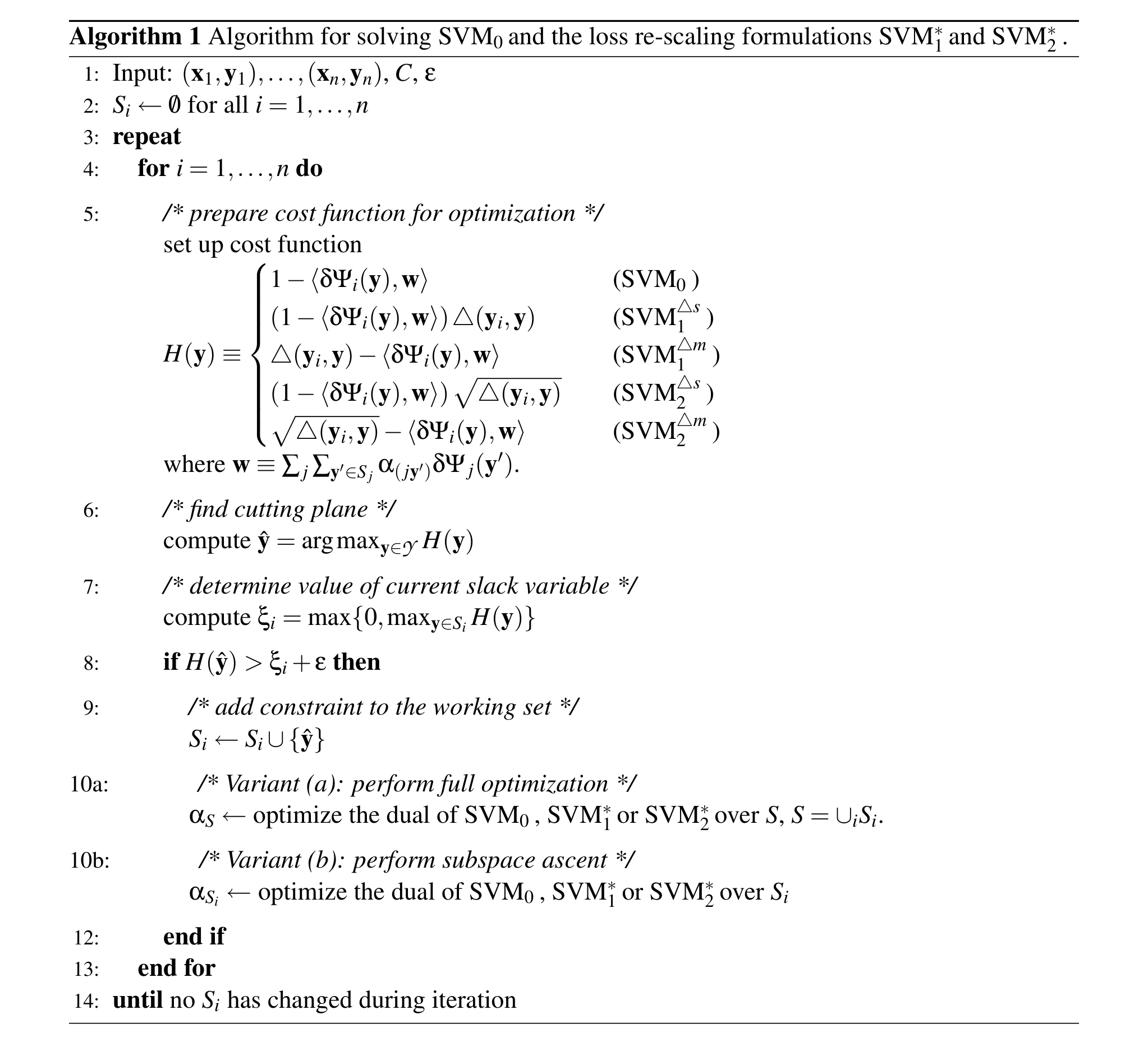
A convenient property of both variants of the cutting plane algorithm is that they have a very general and well-defined interface independent of the choice of $\Psi$ and $\Delta$. To apply the algorithm, it is sufficient to implement the feature mapping $\Psi(\mathbf{x}, \mathbf{y})$ (either explicitly or via a joint kernel function), the loss function $\Delta(\mathbf{y}_i, \mathbf{y})$, as well as the maximization in step 6. All of those, in particular the constraint/cut selection method, are treated as black boxes. While the modeling of $\Psi(\mathbf{x}, \mathbf{y})$ and $\Delta(\mathbf{y}_i, \mathbf{y})$ is typically straightforward, solving the maximization problem for constraint selection typically requires exploiting the structure of $\Psi$ for output spaces that can not be dealt with by exhaustive search.

In the slack re-scaling setting, it turns out that for a given example $(\mathbf{x}_i, \mathbf{y}_i)$ we need to identify the maximum over

$ \hat{\mathbf{y}} \equiv \operatorname{argmax}_{\mathbf{y} \in \mathcal{Y}} { (1 - \langle \mathbf{w}, \delta\Psi_i(\mathbf{y}) \rangle) \Delta(\mathbf{y}_i, \mathbf{y}) }. $

We will discuss several cases for how to solve this problem in Section 4. Typically, it can be solved by an appropriate modification of the prediction problem in Equation (1), which recovers $f$ from $F$. For example, in the case of grammar learning with the $F_1$ score as the loss function via $\Delta(\mathbf{y}_i, \mathbf{y}) = (1 - F_1(\mathbf{y}_i, \mathbf{y}))$, the maximum can be computed using a modified version of the CKY algorithm. More generally, in cases where $\Delta(\mathbf{y}_i, \cdot)$ only takes on a finite number of values, a generic strategy is a two stage approach, where one first computes the maximum over those $\mathbf{y}$ for which the loss is constant, $\Delta(\mathbf{y}_i, \mathbf{y}) = const$, and then maximizes over the finite number of levels.

In the margin re-scaling setting, one needs to solve the maximization problem

$ \hat{\mathbf{y}} \equiv \operatorname{argmax}_{\mathbf{y} \in \mathcal{Y}} { \Delta(\mathbf{y}_i, \mathbf{y}) - \langle \mathbf{w}, \delta\Psi_i(\mathbf{y}) \rangle }.\tag{9} $

In cases where the loss function has an additive decomposition that is compatible with the feature map, one can fold the loss function contribution into the weight vector $\langle \mathbf{w}', \delta\Psi_i(\mathbf{y}) \rangle = \langle \mathbf{w}, \delta\Psi_i(\mathbf{y}) \rangle - \Delta(\mathbf{y}_i, \mathbf{y})$ for some $\mathbf{w}'$. This means the class of cost functions defined by $F(\mathbf{x}, \cdot; \mathbf{w})$ and $F(\mathbf{x}, \cdot; \mathbf{w}) - \Delta(\mathbf{y}, \cdot)$ may actually be identical.

The algorithm for the zero-one loss is a special case of either algorithm. We need to identify the highest scoring $\mathbf{y}$ that is incorrect,

$ \hat{\mathbf{y}} \equiv \operatorname{argmax}_{\mathbf{y} \neq \mathbf{y}_i} { 1 - \langle \mathbf{w}, \delta\Psi_i(\mathbf{y}) \rangle }. $

It is therefore sufficient to identify the best solution $\hat{\mathbf{y}} = \operatorname{argmax}_{\mathbf{y} \in \mathcal{Y}} \langle \mathbf{w}, \Psi(\mathbf{x}i, \mathbf{y}) \rangle$ as well as the second best solution $\tilde{\mathbf{y}} = \operatorname{argmax}{\mathbf{y} \in \mathcal{Y} \setminus \hat{\mathbf{y}}} \langle \mathbf{w}, \Psi(\mathbf{x}_i, \mathbf{y}) \rangle$. The second best solution is necessary to detect margin violations in cases where $\hat{\mathbf{y}} = \mathbf{y}_i$, but $\langle \mathbf{w}, \delta\Psi_i(\tilde{\mathbf{y}}) \rangle < 1$. This means that for all problems where we can solve the inference problem in Equation (1) for the top two $\mathbf{y}$, we can also apply our learning algorithms with the zero-one loss. In the case of grammar learning, for example, we can use any existing parser that returns the two highest scoring parse trees.

We will now proceed by analyzing the presented family of algorithms. In particular, we will show correctness and sparse approximation properties, as well as bounds on the runtime complexity.

3.3 Correctness and Complexity of the Algorithm

What we would like to accomplish first is to obtain a lower bound on the achievable improvement of the dual objective by selecting a single variable $\alpha_{(i\hat{\mathbf{y}})}$ and adding it to the dual problem (cf. step 10 in Algorithm 1). While this is relatively straightforward when using quadratic penalties, the $\text{SVM}1$ formulation introduces an additional complication in the form of upper bounds on non-overlapping subsets of variables, namely the set of variables $\alpha{(i\mathbf{y})}$ in the current working set that correspond to the same training instance. Hence, we may not be able to answer the above question by optimizing over $\alpha_{(i\mathbf{y})}$ alone, but rather have to deal with a larger optimization problem over a whole subspace. In order to derive useful bounds, it suffices to restrict attention to simple one-dimensional families of solutions that are defined by improving an existing solution along a specific direction $\boldsymbol{\eta}$. Proving that one can make sufficient progress along a specific direction, clearly implies that one can make at least that much progress by optimizing over a larger subspace that includes the direction $\boldsymbol{\eta}$. A first step towards executing this idea is the following lemma.

Lemma 10 Let $\mathbf{J}$ be a symmetric, positive semi-definite matrix, and define a concave objective in $\boldsymbol{\alpha}$

$ \Theta(\boldsymbol{\alpha}) = -\frac{1}{2} \boldsymbol{\alpha}^\top \mathbf{J} \boldsymbol{\alpha} + \langle \mathbf{h}, \boldsymbol{\alpha} \rangle, $

which we assume to be bounded from above. Assume that a solution $\boldsymbol{\alpha}^o$ and an optimization direction $\boldsymbol{\eta}$ is given such that $\langle \nabla\Theta(\boldsymbol{\alpha}^o), \boldsymbol{\eta} \rangle > 0$. Then optimizing $\Theta$ starting from $\boldsymbol{\alpha}^o$ along the chosen direction $\boldsymbol{\eta}$ will increase the objective by

$ \max_{\beta > 0} { \Theta(\boldsymbol{\alpha}^o + \beta \boldsymbol{\eta}) } - \Theta(\boldsymbol{\alpha}^o) = \frac{1}{2} \frac{\langle \nabla\Theta(\boldsymbol{\alpha}^o), \boldsymbol{\eta} \rangle^2}{\boldsymbol{\eta}^\top \mathbf{J} \boldsymbol{\eta}} > 0. $

Proof The difference obtained by a particular $\beta$ is given by

$ \delta\Theta(\beta) \equiv \beta \left[ \langle \nabla\Theta(\boldsymbol{\alpha}^o), \boldsymbol{\eta} \rangle - \frac{\beta}{2} \boldsymbol{\eta}^\top \mathbf{J} \boldsymbol{\eta} \right], $

as can be verified by elementary algebra. Solving for $\beta$ one arrives at

$ \frac{d}{d\beta} \delta\Theta = 0 \iff \beta^* = \frac{\langle \nabla\Theta(\boldsymbol{\alpha}^o), \boldsymbol{\eta} \rangle}{\boldsymbol{\eta}^\top \mathbf{J} \boldsymbol{\eta}}. $

Notice that this requires $\boldsymbol{\eta}^\top \mathbf{J} \boldsymbol{\eta} > 0$. Obviously, the positive semi-definiteness of $\mathbf{J}$ guarantees $\boldsymbol{\eta}^\top \mathbf{J} \boldsymbol{\eta} \ge 0$ for any $\boldsymbol{\eta}$. Moreover $\boldsymbol{\eta}^\top \mathbf{J} \boldsymbol{\eta} = 0$ together with $\langle \nabla\Theta(\boldsymbol{\alpha}^o), \boldsymbol{\eta} \rangle > 0$ would imply that $\lim_{\beta \to \infty} \Theta(\boldsymbol{\alpha}^o + \beta \boldsymbol{\eta}) = \infty$, which is in contradiction with the assumption that $\Theta$ is bounded. Plugging the value for $\beta^*$ back into the above expression for $\delta\Theta$ yields the claim.

Corollary 11 Under the same assumption as in Lemma 10 and for the special case of an optimization direction $\boldsymbol{\eta} = \mathbf{e}_r$, the objective improves by

$ \delta\Theta(\beta^*) = \frac{1}{2 J_{rr}} \left( \frac{\partial \Theta}{\partial \alpha_r} \right)^2 > 0. $

Proof Notice that $\boldsymbol{\eta} = \mathbf{e}r$ implies $\langle \nabla\Theta, \boldsymbol{\eta} \rangle = \frac{\partial \Theta}{\partial \alpha_r}$ and $\boldsymbol{\eta}^\top \mathbf{J} \boldsymbol{\eta} = J{rr}$.

Corollary 12 Under the same assumptions as in Lemma 10 and enforcing the constraint $\beta \le D$ for some $D > 0$, the objective improves by

$ \max_{0 < \beta \le D} { \Theta(\boldsymbol{\alpha}^o + \beta \boldsymbol{\eta}) } - \Theta(\boldsymbol{\alpha}^o) = \begin{cases} \frac{\langle \nabla\Theta(\boldsymbol{\alpha}^o), \boldsymbol{\eta} \rangle^2}{2 \boldsymbol{\eta}^\top \mathbf{J} \boldsymbol{\eta}} & \text{if } \langle \nabla\Theta(\boldsymbol{\alpha}^o), \boldsymbol{\eta} \rangle \le D \boldsymbol{\eta}^\top \mathbf{J} \boldsymbol{\eta} \ D \langle \nabla\Theta(\boldsymbol{\alpha}^o), \boldsymbol{\eta} \rangle - \frac{D^2}{2} \boldsymbol{\eta}^\top \mathbf{J} \boldsymbol{\eta} & \text{otherwise} \end{cases} $

Moreover, the improvement can be upper bounded by

$ \max_{0 < \beta \le D} { \Theta(\boldsymbol{\alpha}^o + \beta \boldsymbol{\eta}) } - \Theta(\boldsymbol{\alpha}^o) \ge \frac{1}{2} \min \left{ D, \frac{\langle \nabla\Theta(\boldsymbol{\alpha}^o), \boldsymbol{\eta} \rangle}{\boldsymbol{\eta}^\top \mathbf{J} \boldsymbol{\eta}} \right} \langle \nabla\Theta(\boldsymbol{\alpha}^o), \boldsymbol{\eta} \rangle. $

Proof We distinguish two cases of either $\beta^* \le D$ or $\beta^* > D$. In the first case, we can simple apply lemma 10 since the additional constraint is inactive and does not change the solution. In the second case, the concavity of $\Theta$ implies that $\beta = D$ achieves the maximum of $\delta\Theta$ over the constrained range. Plugging in this result for $\beta^*$ into $\delta\Theta$ yields the second case in the claim.

Finally, the bound is obtained by exploiting that in the second case

$ \beta^* > D \iff D < \frac{\langle \nabla\Theta(\boldsymbol{\alpha}^o), \boldsymbol{\eta} \rangle}{\boldsymbol{\eta}^\top \mathbf{J} \boldsymbol{\eta}}. $

Replacing one of the $D$ factors in the $D^2$ term of the second case with this bound yields an upper bound. The first (exact) case and the bound in the second case can be compactly combined as shown in the formula of the claim.

Corollary 13 Under the same assumption as in Corollary 12 and for the special case of a single-coordinate optimization direction $\boldsymbol{\eta} = \mathbf{e}_r$, the objective improves at least by

$ \max_{0 < \beta \le D} \Theta(\boldsymbol{\alpha}^o + \beta \mathbf{e}r) - \Theta(\boldsymbol{\alpha}^o) \ge \frac{1}{2} \min \left{ D, \frac{\frac{\partial \Theta}{\partial \alpha_r}(\boldsymbol{\alpha}^o)}{J{rr}} \right} \frac{\partial \Theta}{\partial \alpha_r}(\boldsymbol{\alpha}^o) $

Proof Notice that $\boldsymbol{\eta} = \mathbf{e}r$ implies $\langle \nabla\Theta, \boldsymbol{\eta} \rangle = \frac{\partial \Theta}{\partial \alpha_r}$ and $\boldsymbol{\eta}^\top \mathbf{J} \boldsymbol{\eta} = J{rr}$.

We now apply the above lemma and corollaries to the four different SVM formulations, starting with the somewhat simpler squared penalty case.

Proposition 14 ($\text{SVM}_2^{\Delta s}$) For $\text{SVM}_2^{\Delta s}$ step 10 in Algorithm 1 the improvement $\delta\Theta$ of the dual objective is lower bounded by

$ \delta\Theta \ge \frac{1}{2} \frac{\varepsilon^2}{\Delta_i R_i^2 + \frac{n}{C}}, \quad \text{where } \Delta_i \equiv \max_{\mathbf{y}} { \Delta(\mathbf{y}i, \mathbf{y}) } \text{ and } R_i \equiv \max{\mathbf{y}} { |\delta\Psi_i(\mathbf{y})| }. $

Proof Using the notation in Algorithm 1 one can apply Corollary 11 with multi-index $r = (i\hat{\mathbf{y}})$, $\mathbf{h} = \mathbf{1}$, and $\mathbf{J}$ such that

$ J_{(i\hat{\mathbf{y}})(j\mathbf{y})} = \langle \delta\Psi_i(\hat{\mathbf{y}}), \delta\Psi_j(\mathbf{y}) \rangle + \frac{\delta(i, j) n}{C \sqrt{\Delta(\mathbf{y}_i, \hat{\mathbf{y}})} \sqrt{\Delta(\mathbf{y}_i, \mathbf{y})}}. $

Notice that the partial derivative of $\Theta$ with respect to $\alpha_{(i\hat{\mathbf{y}})}$ is given by

$ \frac{\partial \Theta}{\partial \alpha_{(i\hat{\mathbf{y}})}}(\boldsymbol{\alpha}^o) = 1 - \sum_{j, \mathbf{y}} \alpha^o_{(j\mathbf{y})} J_{(i\hat{\mathbf{y}})(j\mathbf{y})} = 1 - \langle \mathbf{w}^*, \delta\Psi_i(\hat{\mathbf{y}}) \rangle - \frac{\xi_i^*}{\sqrt{\Delta(\mathbf{y}_i, \hat{\mathbf{y}})}}, $

since the optimality equations for the primal variables yield the identities

$ \mathbf{w}^* = \sum_{j, \mathbf{y}} \alpha^o_{(j\mathbf{y})} \delta\Psi_j(\mathbf{y}), \quad \text{and} \quad \xi_i^* = \sum_{\mathbf{y} \neq \mathbf{y}i} \frac{n \alpha^o{(i\mathbf{y})}}{C \sqrt{\Delta(\mathbf{y}_i, \mathbf{y})}}. $

Now, applying the condition of step 10, namely $\sqrt{\Delta(\mathbf{y}_i, \hat{\mathbf{y}})} (1 - \langle \mathbf{w}^*, \delta\Psi_i(\hat{\mathbf{y}}) \rangle) > \xi_i^* + \varepsilon$, leads to the bound

$ \frac{\partial \Theta}{\partial \alpha_{(i\hat{\mathbf{y}})}}(\boldsymbol{\alpha}^o) \ge \frac{\varepsilon}{\sqrt{\Delta(\mathbf{y}_i, \hat{\mathbf{y}})}}. $

Finally, $J_{rr} = |\delta\Psi_i(\hat{\mathbf{y}})|^2 + \frac{n}{C \Delta(\mathbf{y}_i, \hat{\mathbf{y}})}$ and inserting this expression and the previous bound into the expression from Corollary 11 yields

$ \frac{1}{2 J_{rr}} \left( \frac{\partial \Theta}{\partial \alpha_{(i\hat{\mathbf{y}})}} \right)^2 \ge \frac{\varepsilon^2}{2 \left( \Delta(\mathbf{y}_i, \hat{\mathbf{y}}) |\delta\Psi_i(\hat{\mathbf{y}})|^2 + \frac{n}{C} \right)} \ge \frac{\varepsilon^2}{2 \left( \Delta_i R_i^2 + \frac{n}{C} \right)}. $

The claim follows by observing that jointly optimizing over a set of variables that include $\alpha_r$ can only further increase the value of the dual objective.

Proposition 15 ($\text{SVM}_2^{\Delta m}$) For $\text{SVM}_2^{\Delta m}$ step 10 in Algorithm 1 the improvement $\delta\Theta$ of the dual objective is lower bounded by

$ \delta\Theta \ge \frac{1}{2} \frac{\varepsilon^2}{R_i^2 + \frac{n}{C}}, \quad \text{where} \quad R_i = \max_{\mathbf{y}} |\delta\Psi_i(\mathbf{y})|. $

Proof By re-defining $\delta\tilde{\Psi}_i(\mathbf{y}) \equiv \frac{\delta\Psi_i(\mathbf{y})}{\sqrt{\Delta(\mathbf{y}_i, \mathbf{y})}}$ we are back to Proposition 14 with

$ \max_{\mathbf{y}} {\Delta(\mathbf{y}_i, \mathbf{y}) |\delta\tilde{\Psi}i(\mathbf{y})|^2} = \max{\mathbf{y}} {|\delta\Psi_i(\mathbf{y})|^2} = R_i^2, $

since

$ \langle \mathbf{w}, \delta\Psi_i(\mathbf{y}) \rangle \ge \sqrt{\Delta(\mathbf{y}_i, \mathbf{y})} - \xi_i \Longleftrightarrow \langle \mathbf{w}, \delta\tilde{\Psi}_i(\mathbf{y}) \rangle \ge 1 - \frac{\xi_i}{\sqrt{\Delta(\mathbf{y}_i, \mathbf{y})}}. $

$\blacksquare$

Proposition 16 ($\text{SVM}_1^{\Delta s}$) For $\text{SVM}_1^{\Delta s}$ step 10 in Algorithm 1 the improvement $\delta\Theta$ of the dual objective is lower bounded by

$ \delta\Theta \ge \min \left{ \frac{C\varepsilon}{2n}, \frac{\varepsilon^2}{8\bar{\Delta}_i^2 R_i^2} \right} \quad \text{where} \quad \bar{\Delta}i = \max{\mathbf{y}} {\Delta(\mathbf{y}i, \mathbf{y})} \text{ and } R_i = \max{\mathbf{y}} {|\delta\Psi_i(\mathbf{y})|}. $

Proof

Case I: If the working set does not contain an element $(i\mathbf{y})$, then we can optimize over $\alpha_{(i\hat{\mathbf{y}})}$ under the constraint that $\alpha_{(i\hat{\mathbf{y}})} \le \Delta(\mathbf{y}_i, \hat{\mathbf{y}}) \frac{C}{n} = D$. Notice that

$ \frac{\partial \Theta}{\partial \alpha_{(i\hat{\mathbf{y}})}} (\boldsymbol{\alpha}^o) = 1 - \langle \mathbf{w}^*, \delta\Psi_i(\hat{\mathbf{y}}) \rangle > \frac{\xi_i^* + \varepsilon}{\Delta(\mathbf{y}_i, \hat{\mathbf{y}})} \ge \frac{\varepsilon}{\Delta(\mathbf{y}_i, \hat{\mathbf{y}})}, $

where the first inequality follows from the pre-condition for selecting $(i\hat{\mathbf{y}})$ and the last one from $\xi_i^* \ge 0$. Moreover, notice that $J_{(i\hat{\mathbf{y}})(i\hat{\mathbf{y}})} \le R_i^2$. Evoking Corollary 13 with the obvious identifications yields

$ \delta\Theta \ge \frac{1}{2} \min \left{ D, \frac{1}{J_{rr}} \frac{\partial \Theta}{\partial \alpha_{(i\hat{\mathbf{y}})}} (\boldsymbol{\alpha}^o) \right} \frac{\partial \Theta}{\partial \alpha_{(i\hat{\mathbf{y}})}} (\boldsymbol{\alpha}^o) > \frac{1}{2} \min \left{ \frac{\Delta(\mathbf{y}_i, \hat{\mathbf{y}})C}{n}, \frac{\varepsilon}{\Delta(\mathbf{y}_i, \hat{\mathbf{y}}) R_i^2} \right} \frac{\varepsilon}{\Delta(\mathbf{y}_i, \hat{\mathbf{y}})} = \min \left{ \frac{C\varepsilon}{2n}, \frac{\varepsilon^2}{2R_i^2 \Delta(\mathbf{y}_i, \hat{\mathbf{y}})^2} \right} $

The second term can be further bounded to yield the claim.

Case II: If there are already active constraints for instance $\mathbf{x}i$ in the current working set, i.e. $S_i \neq \emptyset$, then we may need to reduce dual variables $\alpha{(i\mathbf{y})}$ in order to get some slack for increasing the newly added $\alpha_{(i\hat{\mathbf{y}})}$. We thus investigate search directions $\boldsymbol{\eta}$ such that $\eta_{(i\hat{\mathbf{y}})} = 1$, $\eta_{(i\mathbf{y})} = -\frac{\alpha_{(i\mathbf{y})}}{\Delta(\mathbf{y}i, \hat{\mathbf{y}})} \frac{n}{C} \le 0$ for $\mathbf{y} \in S_i$, and $\eta{(j\mathbf{y}')} = 0$ in all other cases. For such $\boldsymbol{\eta}$, we guarantee that $\boldsymbol{\alpha}^o + \beta\boldsymbol{\eta} \ge 0$ since $\beta \le \frac{C}{n}\Delta(\mathbf{y}_i, \hat{\mathbf{y}})$. In finding a suitable direction to derive a good bound, we have two (possibly conflicting) goals. First of all, we want the directional derivative to be positively bounded away from zero. Notice that

$ \langle \nabla\Theta(\boldsymbol{\alpha}^o), \boldsymbol{\eta} \rangle = \sum_{\mathbf{y}} \eta_{(i\mathbf{y})} (1 - \langle \mathbf{w}^*, \delta\Psi_i(\mathbf{y}) \rangle). $

Furthermore, by the restrictions imposed on $\boldsymbol{\eta}$, $\eta_{(i\mathbf{y})} < 0$ implies that the respective constraint is active and hence $\Delta(\mathbf{y}_i, \mathbf{y}) (1 - \langle \mathbf{w}^*, \delta\Psi_i(\mathbf{y}) \rangle) = \xi_i^*$. Moreover the pre-condition of step 10 ensures that $\Delta(\mathbf{y}_i, \hat{\mathbf{y}}) (1 - \langle \mathbf{w}^*, \delta\Psi_i(\hat{\mathbf{y}}) \rangle) = \xi_i^* + \delta$ where $\delta \ge \varepsilon > 0$. Hence

$ \langle \nabla\Theta(\boldsymbol{\alpha}^o), \boldsymbol{\eta} \rangle = \frac{\xi_i^*}{\Delta(\mathbf{y}i, \hat{\mathbf{y}})} \left( 1 - \frac{n}{C} \sum{\mathbf{y}} \frac{\alpha_{(i\mathbf{y})}^o}{\Delta(\mathbf{y}_i, \mathbf{y})} \right) + \frac{\delta}{\Delta(\mathbf{y}_i, \hat{\mathbf{y}})} \ge \frac{\varepsilon}{\Delta(\mathbf{y}_i, \hat{\mathbf{y}})}. $

The second goal is to make sure the curvature along the chosen direction is not too large.

$ \boldsymbol{\eta}^\top J \boldsymbol{\eta} = J_{(i\hat{\mathbf{y}})(i\hat{\mathbf{y}})} - 2 \sum_{\mathbf{y} \neq \hat{\mathbf{y}}} \frac{\alpha_{(i\mathbf{y})}^o}{\Delta(\mathbf{y}i, \hat{\mathbf{y}})} \frac{n}{C} J{(i\hat{\mathbf{y}})(i\mathbf{y})} + \sum_{\mathbf{y} \neq \hat{\mathbf{y}}} \sum_{\mathbf{y}' \neq \hat{\mathbf{y}}} \frac{\alpha_{(i\mathbf{y})}^o}{\Delta(\mathbf{y}i, \hat{\mathbf{y}})} \frac{n}{C} \frac{\alpha{(i\mathbf{y}')}^o}{\Delta(\mathbf{y}i, \hat{\mathbf{y}})} \frac{n}{C} J{(i\mathbf{y})(i\mathbf{y}')} $

$ \le R_i^2 + 2 \frac{n R_i^2}{C \Delta(\mathbf{y}i, \hat{\mathbf{y}})} \sum{\mathbf{y} \neq \hat{\mathbf{y}}} \alpha_{(i\mathbf{y})}^o + \frac{n^2 R_i^2}{C^2 \Delta(\mathbf{y}i, \hat{\mathbf{y}})^2} \sum{\mathbf{y} \neq \hat{\mathbf{y}}} \sum_{\mathbf{y}' \neq \hat{\mathbf{y}}} \alpha_{(i\mathbf{y})}^o \alpha_{(i\mathbf{y}')}^o $

$ \le R_i^2 + 2 \frac{R_i^2 \bar{\Delta}_i}{\Delta(\mathbf{y}_i, \hat{\mathbf{y}})} + \frac{R_i^2 \bar{\Delta}_i^2}{\Delta(\mathbf{y}_i, \hat{\mathbf{y}})^2} \le \frac{4 R_i^2 \bar{\Delta}_i^2}{\Delta(\mathbf{y}_i, \hat{\mathbf{y}})^2}. $

This follows from the fact that $\sum_{\mathbf{y} \neq \hat{\mathbf{y}}} \alpha_{(i\mathbf{y})}^o \le \bar{\Delta}i \sum{\mathbf{y} \neq \hat{\mathbf{y}}} \frac{\alpha_{(i\mathbf{y})}^o}{\Delta(\mathbf{y}_i, \mathbf{y})} \le \frac{C\bar{\Delta}_i}{n}$. Evoking Corollary 12 yields

$ \delta\Theta \ge \frac{1}{2} \min \left{ D, \frac{\langle \nabla\Theta(\boldsymbol{\alpha}^o), \boldsymbol{\eta} \rangle}{\boldsymbol{\eta}^\top J \boldsymbol{\eta}} \right} \langle \nabla\Theta(\boldsymbol{\alpha}^o), \boldsymbol{\eta} \rangle \ge \frac{1}{2} \min \left{ \frac{\Delta(\mathbf{y}_i, \hat{\mathbf{y}})C}{n}, \frac{\frac{\varepsilon}{\Delta(\mathbf{y}_i, \hat{\mathbf{y}})}}{\frac{4R_i^2 \bar{\Delta}_i^2}{\Delta(\mathbf{y}_i, \hat{\mathbf{y}})^2}} \right} \frac{\varepsilon}{\Delta(\mathbf{y}_i, \hat{\mathbf{y}})} = \min \left{ \frac{C\varepsilon}{2n}, \frac{\varepsilon^2}{8R_i^2 \bar{\Delta}_i^2} \right} $

$\blacksquare$

Proposition 17 ($\text{SVM}_1^{\Delta m}$) For $\text{SVM}_1^{\Delta m}$ step 10 in Algorithm 1 the improvement $\delta\Theta$ of the dual objective is lower bounded by

$ \delta\Theta \ge \frac{\varepsilon^2}{8R_i^2}, \quad \text{where} \quad R_i = \max_{\mathbf{y}} |\delta\Psi_i(\mathbf{y})|. $

Proof By re-defining $\delta\tilde{\Psi}_i(\mathbf{y}) \equiv \frac{\delta\Psi_i(\mathbf{y})}{\Delta(\mathbf{y}_i, \mathbf{y})}$ we are back to Proposition 16 with

$ \max_{\mathbf{y}} {\Delta(\mathbf{y}_i, \mathbf{y})^2 |\delta\tilde{\Psi}i(\mathbf{y})|^2} = \max{\mathbf{y}} {|\delta\Psi_i(\mathbf{y})|^2} = R_i^2, $

since

$ \langle \mathbf{w}, \delta\Psi_i(\mathbf{y}) \rangle \ge \Delta(\mathbf{y}_i, \mathbf{y}) - \xi_i \Longleftrightarrow \langle \mathbf{w}, \delta\tilde{\Psi}_i(\mathbf{y}) \rangle \ge 1 - \frac{\xi_i}{\Delta(\mathbf{y}_i, \mathbf{y})}. $

$\blacksquare$

This leads to the following polynomial bound on the maximum size of $S$.

Theorem 18 With $\bar{R} = \max_i R_i$, $\bar{\Delta} = \max_i \bar{\Delta}_i$ and for a given $\varepsilon > 0$, Algorithm 1 terminates after incrementally adding at most

$ \max \left{ \frac{2n\bar{\Delta}}{\varepsilon}, \frac{8C\bar{\Delta}^3 \bar{R}^2}{\varepsilon^2} \right}, \quad \max \left{ \frac{2n\bar{\Delta}}{\varepsilon}, \frac{8C\bar{\Delta}\bar{R}^2}{\varepsilon^2} \right}, \quad \frac{C\bar{\Delta}^2 \bar{R}^2 + n\bar{\Delta}}{\varepsilon^2} \quad \text{and} \quad \frac{C\bar{\Delta}\bar{R}^2 + n\bar{\Delta}}{\varepsilon^2} $

constraints to the working set $S$ for the $\text{SVM}_1^{\Delta s}$, $\text{SVM}_1^{\Delta m}$, $\text{SVM}_2^{\Delta s}$ and $\text{SVM}_2^{\Delta m}$ respectively.

Proof With $S = \emptyset$ the optimal value of the dual is $0$. In each iteration a constraint is added that is violated by at least $\varepsilon$, provided such a constraint exists. After solving the $S$-relaxed QP in step 10, the objective will increase by at least the amounts suggested by Propositions 16, 17, 14 and 15 respectively. Hence after $t$ constraints, the dual objective will be at least $t$ times these increments. The result follows from the fact that the dual objective is upper bounded by the minimum of the primal, which in turn can be bounded by $C\bar{\Delta}$ and $\frac{1}{2} C\bar{\Delta}$ for $\text{SVM}_1^*$ and $\text{SVM}_2^*$ respectively. $\blacksquare$

Note that the number of constraints in $S$ does not depend on $|\mathcal{Y}|$. This is crucial, since $|\mathcal{Y}|$ is exponential or infinite for many interesting problems. For problems where step 6 can be computed in polynomial time, the overall algorithm has a runtime polynomial in $n, \bar{R}, \bar{\Delta}, 1/\varepsilon$, since at least one constraint will be added while cycling through all $n$ instances and since step 10 is polynomial. This shows that the algorithm considers only a small number of constraints, if one allows an extra $\varepsilon$ slack, and that the solution is correct up to an approximation that depends on the precision parameter $\varepsilon$. The upper bound on the number of active constraints in such an approximate solution depends on the chosen representation, more specifically, we need to upper bound the difference vectors $|\Psi(\mathbf{x}_i, \mathbf{y}) - \Psi(\mathbf{x}_i, \bar{\mathbf{y}})|^2$ for arbitrary $\mathbf{y}, \bar{\mathbf{y}} \in \mathcal{Y}$. In the following, we will thus make sure that suitable upper bounds are available.

4. Specific Problems and Special Cases

Section Summary: The section explores special cases of a general structured prediction framework by addressing three practical issues for each one: how to construct joint feature maps that combine inputs and outputs, how to efficiently solve the maximization step over possible labels, and how to bound differences between those feature maps so that algorithmic complexity can be controlled. It first works through standard multiclass classification, showing that a simple winner-takes-all rule can be expressed using tensor-product features and that exhaustive search plus a straightforward norm bound suffice when the number of classes is small. It then generalizes the approach to richer, kernel-defined output features that capture similarities among labels while preserving the same computational advantages.

In the sequel, we will discuss a number of interesting special cases of the general scenario outlined in the previous section. To model each particular problem and to be able to run the algorithm and bound its complexity, we need to examine the following three questions for each case:

• Modeling: How can we define suitable feature maps $\Psi(\mathbf{x}, \mathbf{y})$ for specific problems?
• Algorithms: How can we compute the required maximization over $\mathcal{Y}$ for given $\mathbf{x}$?
• Sparseness: How can we bound $|\Psi(\mathbf{x}, \mathbf{y}) - \Psi(\mathbf{x}, \mathbf{y}')|$?

4.1 Multiclass Classification

A special case of Equation (1) is winner-takes-all (WTA) multiclass classification, where $\mathcal{Y} = {\mathbf{y}_1, \dots, \mathbf{y}_K}$ and $\mathbf{w} = (\mathbf{v}_1^\top, \dots, \mathbf{v}_K^\top)^\top$ is a stack of vectors, $\mathbf{v}_k$ being a weight vector associated with the $k$-th class $\mathbf{y}_k$. The WTA rule is given by

$ f(\mathbf{x}) = \arg\max_{\mathbf{y}_k \in \mathcal{Y}} F(\mathbf{x}, \mathbf{y}; \mathbf{w}), \quad F(\mathbf{x}, \mathbf{y}_k; \mathbf{w}) = \langle \mathbf{v}_k, \Phi(\mathbf{x}) \rangle.\tag{10} $

Here $\Phi(\mathbf{x}) \in \mathbb{R}^D$ denotes an arbitrary feature representation of the inputs, which in many cases may be defined implicitly via a kernel function.

4.1.1 Modeling

The above decision rule can be equivalently represented by making use of a joint feature map as follows. First of all, we define the canonical (binary) representation of labels $\mathbf{y} \in \mathcal{Y}$ by unit vectors

$ \Lambda^c(\mathbf{y}) \equiv (\delta(\mathbf{y}_1, \mathbf{y}), \delta(\mathbf{y}_2, \mathbf{y}), \dots, \delta(\mathbf{y}_K, \mathbf{y}))^\top \in {0, 1}^K,\tag{11} $

so that $\langle \Lambda^c(\mathbf{y}), \Lambda^c(\mathbf{y}') \rangle = \delta(\mathbf{y}, \mathbf{y}')$. It will turn out to be convenient to use direct tensor products $\otimes$ to combine feature maps over $\mathcal{X}$ and $\mathcal{Y}$. In general, we thus define the $\otimes$-operation in the following manner

$ \otimes : \mathbb{R}^D \times \mathbb{R}^K \to \mathbb{R}^{D \cdot K}, \quad (\mathbf{a} \otimes \mathbf{b})_{i + (j-1)D} \equiv a_i \cdot b_j. $

Now we can define a joint feature map for the multiclass problem by

$ \Psi(\mathbf{x}, \mathbf{y}) \equiv \Phi(\mathbf{x}) \otimes \Lambda^c(\mathbf{y}).\tag{12} $

It is is easy to show that this results in an equivalent formulation of the multiclass WTA as expressed in the following proposition.

Proposition 19 $F(\mathbf{x}, \mathbf{y}; \mathbf{w}) = \langle \mathbf{w}, \Psi(\mathbf{x}, \mathbf{y}) \rangle$, where $F$ is defined in Equation (10) and $\Psi$ in Equation (12).

Proof For all $\mathbf{y}k \in \mathcal{Y}$: $\langle \mathbf{w}, \Psi(\mathbf{x}, \mathbf{y}k) \rangle = \sum{r=1}^{D \cdot K} w_r \psi_r(\mathbf{x}, \mathbf{y}k) = \sum{j=1}^K \sum{d=1}^D v_{jd} \phi_d(\mathbf{x}) \delta(j, k) = \sum_{d=1}^D v_{kd} \phi_d(\mathbf{x}) = \langle \mathbf{v}_k, \Phi(\mathbf{x}) \rangle$.

4.1.2 Algorithms

It is usually assumed that the number of classes $K$ in simple multiclass problems is small enough, so that an exhaustive search can be performed to maximize any objective over $\mathcal{Y}$. Similarly, we can find the second best $\mathbf{y} \in \mathcal{Y}$.

4.1.3 Sparseness

In order to bound the norm of the difference feature vectors, we prove the following simple result.

Proposition 20 Define $R_i \equiv |\Phi(\mathbf{x}_i)|$. Then $|\Psi(\mathbf{x}_i, \mathbf{y}) - \Psi(\mathbf{x}_i, \mathbf{y}')|^2 \le 2R_i^2$.

Proof

$ |\Psi(\mathbf{x}_i, \mathbf{y}) - \Psi(\mathbf{x}_i, \mathbf{y}')|^2 \le |\Psi(\mathbf{x}_i, \mathbf{y})|^2 + |\Psi(\mathbf{x}_i, \mathbf{y}')|^2 = 2|\Phi(\mathbf{x}_i)|^2, $

where the first step follows from the Cauchy-Schwarz inequality and the second step exploits the sparseness of $\Lambda^c$. $\blacksquare$

4.2 Multiclass Classification with Output Features

The first generalization we propose is to make use of more interesting output features $\Lambda$ than the canonical representation in Equation (11). Apparently, we could use the same approach as in Equation (12) to define a joint feature function, but use a more general form for $\Lambda$.

4.2.1 Modeling

We first show that for any joint feature map $\Psi$ constructed via the direct tensor product $\otimes$ the following relation holds:

Proposition 21 For $\Psi = \Phi \otimes \Lambda$ the inner product can be written as

$ \langle \Psi(\mathbf{x}, \mathbf{y}), \Psi(\mathbf{x}', \mathbf{y}') \rangle = \langle \Phi(\mathbf{x}), \Phi(\mathbf{x}') \rangle \cdot \langle \Lambda(\mathbf{y}), \Lambda(\mathbf{y}') \rangle. $

Proof By simple algebra

$ \langle \Psi(\mathbf{x}, \mathbf{y}), \Psi(\mathbf{x}', \mathbf{y}') \rangle = \sum_{r=1}^{D \cdot K} \sum_{s=1}^{D \cdot K} \psi_r(\mathbf{x}, \mathbf{y}) \psi_s(\mathbf{x}', \mathbf{y}') = \sum_{d=1}^D \sum_{k=1}^K \sum_{d'=1}^D \sum_{k'=1}^K \phi_d(\mathbf{x}) \lambda_k(\mathbf{y}) \phi_{d'}(\mathbf{x}') \lambda_{k'}(\mathbf{y}') $

$ = \sum_{d=1}^D \sum_{d'=1}^D \phi_d(\mathbf{x}) \phi_{d'}(\mathbf{x}') \sum_{k=1}^K \sum_{k'=1}^K \lambda_k(\mathbf{y}) \lambda_{k'}(\mathbf{y}') = \langle \Phi(\mathbf{x}), \Phi(\mathbf{x}') \rangle \cdot \langle \Lambda(\mathbf{y}), \Lambda(\mathbf{y}') \rangle. $

$\blacksquare$

This implies that for feature maps $\Phi$ that are implicitly defined via kernel functions $K$, $K(\mathbf{x}, \mathbf{x}') \equiv \langle \Phi(\mathbf{x}), \Phi(\mathbf{x}') \rangle$, one can define a joint kernel function as follows:

$ J((\mathbf{x}, \mathbf{y}), (\mathbf{x}', \mathbf{y}')) = \langle \Psi(\mathbf{x}, \mathbf{y}), \Psi(\mathbf{x}', \mathbf{y}') \rangle = \langle \Lambda(\mathbf{y}), \Lambda(\mathbf{y}') \rangle K(\mathbf{x}, \mathbf{x}'). $

Of course, nothing prevents us from expressing the inner product in output space via yet another kernel function $L(\mathbf{y}, \mathbf{y}') = \langle \Lambda(\mathbf{y}), \Lambda(\mathbf{y}') \rangle$. Notice that the kernel $L$ is simply the identity in the standard multiclass case. How can this kernel be chosen in concrete cases? It basically may encode any type of prior knowledge one might have about the similarity between classes. It is illuminating to note the following proposition.

Proposition 22 Define $\Psi(\mathbf{x}, \mathbf{y}) = \Phi(\mathbf{x}) \otimes \Lambda(\mathbf{y})$ with $\Lambda(\mathbf{y}) \in \mathbb{R}^R$; then the discriminant function $F(\mathbf{x}, \mathbf{y}; \mathbf{w})$ can be written as

$ F(\mathbf{x}, \mathbf{y}; \mathbf{w}) = \sum_{r=1}^R \lambda_r(\mathbf{y}) \langle \mathbf{v}_r, \Phi(\mathbf{x}) \rangle, $

where $\mathbf{w} = (\mathbf{v}_1^\top, \dots, \mathbf{v}_R^\top)^\top$ is the stack of vectors $\mathbf{v}_r \in \mathbb{R}^D$, one vector for each basis function of $\Lambda$.

Proof

$ \sum_{r=1}^R \lambda_r(\mathbf{y}) \sum_{d=1}^D v_{rd} \phi_d(\mathbf{x}) = \sum_{r=1}^R \sum_{d=1}^D w_{D \cdot (d-1) + r} \lambda_r(\mathbf{y}) \phi_d(\mathbf{x}) = \langle \mathbf{w}, \Phi(\mathbf{x}) \otimes \Lambda(\mathbf{y}) \rangle $

$ = \langle \mathbf{w}, \Psi(\mathbf{x}, \mathbf{y}) \rangle = F(\mathbf{x}, \mathbf{y}; \mathbf{w}). $

$\blacksquare$

We can give this a simple interpretation: For each output feature $\lambda_r$ a corresponding weight vector $\mathbf{v}_r$ is introduced. The discriminant function can then be represented as a weighted sum of contributions coming from the different features. In particular, in the case of binary features $\Lambda : \mathcal{Y} \to {0, 1}^R$, this will simply be a sum over all contributions $\langle \mathbf{v}_r, \Phi(\mathbf{x}) \rangle$ of features that are active for the class $\mathbf{y}$, i.e. for which $\lambda_r(\mathbf{y}) = 1$.

It is also important to note that the orthogonal representation provides a maximally large hypothesis class and that nothing can be gained in terms of representational power by including additional features.

Corollary 23 Assume a mapping $\Lambda(\mathbf{y}) = (\tilde{\Lambda}(\mathbf{y})^\top, \Lambda^c(\mathbf{y})^\top)^\top$, $\tilde{\Lambda}(\mathbf{y}) \in \mathbb{R}^R$ and define $\tilde{\Psi}(\mathbf{x}, \mathbf{y}) = \Phi(\mathbf{x}) \otimes \Lambda(\mathbf{y})$ and $\Psi(\mathbf{x}, \mathbf{y}) = \Phi(\mathbf{x}) \otimes \Lambda^c(\mathbf{y})$. Now, for every $\tilde{\mathbf{w}}$ there is $\mathbf{w}$ such that $\langle \tilde{\mathbf{w}}, \tilde{\Psi}(\mathbf{x}, \mathbf{y}) \rangle = \langle \mathbf{w}, \Psi(\mathbf{x}, \mathbf{y}) \rangle$ and vice versa.

Proof Applying Proposition 22 twice it follows that

$ \langle \tilde{\mathbf{w}}, \tilde{\Psi}(\mathbf{x}, \mathbf{y}) \rangle = \sum_{r=1}^{R+K} \lambda_r(\mathbf{y}) \langle \tilde{\mathbf{v}}r, \Phi(\mathbf{x}) \rangle = \left\langle \sum{r=1}^{R+K} \lambda_r(\mathbf{y}) \tilde{\mathbf{v}}r, \Phi(\mathbf{x}) \right\rangle = \langle \mathbf{v}{\mathbf{y}}, \Phi(\mathbf{x}) \rangle = \langle \mathbf{w}, \Psi(\mathbf{x}, \mathbf{y}) \rangle. $

where we have defined $\mathbf{v}{\mathbf{y}} = \sum{r=1}^{R+K} \lambda_r(\mathbf{y}) \tilde{\mathbf{v}}_r$. The reverse direction is trivial and requires setting $\tilde{\mathbf{v}}_r = \mathbf{0}$ for $r = 1, \dots, R$. $\blacksquare$

In the light of this corollary, we would like to emphasize that the rationale behind the use of class features is not to increase the representational power of the hypothesis space, but to re-parameterize (or even constrain) the hypothesis space such that a more suitable representation for $\mathcal{Y}$ is produced. We would like to generalize across classes as we want to generalize across input patterns in the standard formulation of classification problems. Obviously, orthogonal representations (corresponding to diagonal kernels) will provide no generalization whatsoever across different classes $\mathbf{y}$. The choice of a good output feature map $\Lambda$ is thus expected to provide an inductive bias, namely that learning can occur across a set of classes sharing a common property.

Let us discuss some special cases of interest.

Classification with Taxonomies Assume that class labels $\mathbf{y}$ are arranged in a taxonomy. We will define a taxonomy as a set of elements $\mathcal{Z} \supseteq \mathcal{Y}$ equipped with a partial order $\prec$. The partially ordered set $(\mathcal{Z}, \prec)$ might, for example, represent a tree or a lattice. Now we can define binary features for classes as follows: Associate one feature $\lambda_{\mathbf{z}}$ with every element in $\mathcal{Z}$ according to

$ \lambda_{\mathbf{z}}(\mathbf{y}) = \begin{cases} 1 & \text{if } \mathbf{y} \prec \mathbf{z} \text{ or } \mathbf{y} = \mathbf{z} \ 0 & \text{otherwise.} \end{cases} $

This includes multiclass classification as a special case of an unordered set $\mathcal{Z} = \mathcal{Y}$. In general, however, the features $\lambda_{\mathbf{z}}$ will be "shared" by all classes below $\mathbf{z}$, e.g. all nodes $\mathbf{y}$ in the subtree rooted at $\mathbf{z}$ in the case of a tree. One may also introduce a relative weight $\beta_{\mathbf{z}}$ for every feature and define a $\beta$-weighted (instead of binary) output feature map $\tilde{\Lambda}$ as $\tilde{\lambda}{\mathbf{z}} = \beta{\mathbf{z}} \lambda_{\mathbf{z}}$. If we reflect upon the implication of this definition in the light of Proposition 22, one observes that this effectively introduces a weight vector $\mathbf{v}_{\mathbf{z}}$ for every element of $\mathcal{Z}$, i.e. for every node in the hierarchy.

Learning with Textual Class Descriptions As a second motivating example, we consider problems where classes are characterized by short glosses, blurbs or other textual descriptions. We would like to exploit the fact that classes sharing some descriptors are likely to be similar, in order to specify a suitable inductive bias. This can be achieved, for example, by associating a feature $\lambda$ with every keyword used to describe classes, in addition to the class identity. Hence standard vector space models like term-frequency of idf representations can be applied to model classes and the inner product $\langle \Lambda(\mathbf{y}), \Lambda(\mathbf{y}') \rangle$ then defines a similarity measure between classes corresponding to the standard cosine-measure used in information retrieval.

Learning with Class Similarities The above example can obviously be generalized to any situation, where we have access to a positive definite similarity function for pairs of classes. To come up with suitable similarity functions is part of the domain model—very much like determining a good representation of the inputs—and we assume here that it is given.

4.2.2 Algorithms

As in the multiclass case, we assume that the number of classes is small enough to perform an exhaustive search.

4.2.3 Sparseness

Proposition 20 can be generalized in the following way:

Proposition 24 Define $R_i \equiv |\Phi(\mathbf{x}i)|$ and $S \equiv \max{\mathbf{y} \in \mathcal{Y}} |\Lambda(\mathbf{y})|$ then $|\Psi(\mathbf{x}_i, \mathbf{y}) - \Psi(\mathbf{x}_i, \mathbf{y}')|^2 \le 2R_i^2 S^2$ for all $\mathbf{y}, \mathbf{y}' \in \mathcal{Y}$.

Proof $\langle \Psi(\mathbf{x}_i, \mathbf{y}), \Psi(\mathbf{x}_i, \mathbf{y}) \rangle = |\Phi(\mathbf{x}_i)|^2 \cdot |\Lambda(\mathbf{y})|^2 \le R_i^2 S^2$. In the last step, we have used Proposition 21. $\blacksquare$

4.3 Label Sequence Learning

The next problem we would like to formulate in the joint feature map framework is the problem of label sequence learning, or sequence segmentation/annotation. Here, the goal is to predict a label sequence $\mathbf{y} = (y^1, \dots, y^T)$ for a given observation sequence $\mathbf{x} = (\mathbf{x}^1, \dots, \mathbf{x}^T)$. In order to simplify the presentation, let us assume all sequences are of the same length $T$. Let us denote by $\Sigma$ the set of possible labels for each individual variable $y^t$, i.e. $\mathcal{Y} = \Sigma^T$. Hence each sequence of labels is considered to be a class of its own, resulting in a multiclass classification problem with $|\Sigma|^T$ different classes. To model label sequence learning in this manner would of course not be very useful, if one were to apply standard multiclass classification methods. However, this can be overcome by an appropriate definition of the discriminant function.

4.3.1 Modeling

Inspired by hidden Markov model (HMM) type of interactions, we propose to define $\Psi$ to include interactions between input features and labels via multiple copies of the input features as well as features that model interactions between nearby label variables. It is perhaps most intuitive to start from the discriminant function

$ F(\mathbf{x}, \mathbf{y}; \mathbf{w}) = \sum_{t=1}^T \sum_{\sigma \in \Sigma} \langle \bar{\mathbf{w}}\sigma, \Phi(\mathbf{x}^t) \rangle \delta(y^t, \sigma) + \eta \sum{t=1}^{T-1} \sum_{\sigma \in \Sigma} \sum_{\bar{\sigma} \in \Sigma} \hat{w}_{\sigma, \bar{\sigma}} \delta(y^t, \sigma) \delta(y^{t+1}, \bar{\sigma}) $

$ = \left\langle \bar{\mathbf{w}}, \sum_{t=1}^T \Phi(\mathbf{x}^t) \otimes \Lambda^c(y^t) \right\rangle + \eta \left\langle \hat{\mathbf{w}}, \sum_{t=1}^{T-1} \Lambda^c(y^t) \otimes \Lambda^c(y^{t+1}) \right\rangle.\tag{13} $

Here $\mathbf{w} = (\bar{\mathbf{w}}^\top, \hat{\mathbf{w}}^\top)^\top$, $\Lambda^c$ denotes the orthogonal representation of labels over $\Sigma$, and $\eta \ge 0$ is a scaling factor which balances the two types of contributions. It is straightforward to read off the joint feature map implicit in the definition of the HMM discriminant from Equation (13),

$ \Psi(\mathbf{x}, \mathbf{y}) = \begin{pmatrix} \sum_{t=1}^T \Phi(\mathbf{x}^t) \otimes \Lambda^c(y^t) \ \eta \sum_{t=1}^{T-1} \Lambda^c(y^t) \otimes \Lambda^c(y^{t+1}) \end{pmatrix}. $

Notice that similar to the multiclass case, we can apply Proposition 21 in the case of an implicit representation of $\Phi$ via a kernel function $K$ and the inner product between labeled sequences can thus be written as

$ \langle \Psi((\mathbf{x}, \mathbf{y})), \Psi(\bar{\mathbf{x}}, \bar{\mathbf{y}}) \rangle = \sum_{s,t=1}^T \delta(y^t, \bar{y}^s) K(\mathbf{x}^t, \bar{\mathbf{x}}^s) + \eta^2 \sum_{s,t=1}^{T-1} \delta(y^t, \bar{y}^s) \delta(y^{t+1}, \bar{y}^{s+1}).\tag{14} $

A larger family of discriminant functions can be obtained by using more powerful feature functions $\Psi$. We would like to mention three ways of extending the previous HMM discriminant. First of all, one can extract features not just from $\mathbf{x}^t$, but from a window around $\mathbf{x}^t$, e.g. replacing $\Phi(\mathbf{x}^t)$ with $\Phi(\mathbf{x}^{t-r}, \dots, \mathbf{x}^t, \dots, \mathbf{x}^{t+r})$. Since the same input pattern $\mathbf{x}^t$ now occurs in multiple terms, this has been called the use of overlapping features (Lafferty et al., 2001) in the context of label sequence learning. Secondly, it is also straightforward to include higher order label-label interactions beyond pairwise interactions by including higher order tensor terms, for instance, label triplets $\sum_t \Lambda^c(y^t) \otimes \Lambda^c(y^{t+1}) \otimes \Lambda^c(y^{t+2})$, etc. Thirdly, one can also combine higher order $\mathbf{y}$ features with input features, for example, by including terms of the type $\sum_t \Phi(\mathbf{x}^t) \otimes \Lambda^c(y^t) \otimes \Lambda^c(y^{t+1})$.

4.3.2 Algorithms

The maximization of $\langle \mathbf{w}, \Psi(\mathbf{x}_i, \mathbf{y}) \rangle$ over $\mathbf{y}$ can be carried out by dynamic programming, since the cost contributions are additive over sites and contain only linear and nearest neighbor quadratic contributions. In particular, in order to find the best label sequence $\hat{\mathbf{y}} \neq \mathbf{y}_i$, one can perform Viterbi decoding (Forney Jr., 1973; Schwarz and Chow, 1990), which can also determine the second best sequence for the zero-one loss (2-best Viterbi decoding). Viterbi decoding can also be used with other loss functions by computing the maximization for all possible values of the loss function.

4.3.3 Sparseness

Proposition 25 Define $R_i \equiv \max_t |\Phi(\mathbf{x}_i^t)|$; then $|\Psi(\mathbf{x}_i, \mathbf{y}) - \Psi(\mathbf{x}_i, \mathbf{y}')|^2 \le 2T^2(R_i^2 + \eta^2)$.

Proof Notice that $|\Psi(\mathbf{x}_i, \mathbf{y})|^2 = |\sum_t \Phi(\mathbf{x}_i^t) \otimes \Lambda^c(y^t)|^2 + \eta^2 |\sum_t \Lambda^c(y^t) \otimes \Lambda^c(y^{t+1})|^2$. The first squared norm can be upper bounded by

$ \left|\sum_t \Phi(\mathbf{x}_i^t) \otimes \Lambda^c(y^t)\right|^2 = \sum_s \sum_t \langle \Phi(\mathbf{x}_i^s), \Phi(\mathbf{x}_i^t) \rangle \delta(y^s, y^t) \le T^2 R_i^2 $

and the second one by $\eta^2 T^2$, which yields the claim. $\blacksquare$

4.4 Sequence Alignment

Next we show how to apply the proposed algorithm to the problem of learning to align sequences $\mathbf{x} \in \Sigma^*$, where $\Sigma^*$ is the set of all strings over some finite alphabet $\Sigma$. For a given pair of sequences $\mathbf{x} \in \Sigma^*$ and $\mathbf{y} \in \Sigma^*$, alignment methods like the Smith-Waterman algorithm select the sequence of operations (e.g. insertion, substitution) that transforms $\mathbf{x}$ into $\mathbf{y}$ and that maximizes a linear objective function

$ \hat{\mathbf{a}}(\mathbf{x}, \mathbf{y}) = \arg\max_{\mathbf{a} \in \mathcal{A}} \langle \mathbf{w}, \Psi(\mathbf{x}, \mathbf{y}, \mathbf{a}) \rangle $

that is parameterized by the operation scores $\mathbf{w}$. $\Psi(\mathbf{x}, \mathbf{y}, \mathbf{a})$ is the histogram of alignment operations. The value of $\langle \mathbf{w}, \Psi(\mathbf{x}, \mathbf{y}, \hat{\mathbf{a}}(\mathbf{x}, \mathbf{y})) \rangle$ can be used as a measure of similarity between $\mathbf{x}$ and $\mathbf{y}$. It is the score of the highest scoring sequence of operations that transforms $\mathbf{x}$ into $\mathbf{y}$. Such alignment models are used, for example, to measure the similarity of two protein sequences.

4.4.1 Modeling

In order to learn the score vector $\mathbf{w}$ we use training data of the following type. For each native sequence $\mathbf{x}_i$ there is a most similar homologous sequence $\mathbf{y}_i$ along with the optimal alignment $\mathbf{a}_i$. In addition we are given a set of decoy sequences $\mathbf{y}_i^t$, $t = 1, \dots, k$ with unknown alignments. Note that this data is more restrictive than what Ristad and Yianilos (1997) consider in their generative modeling approach. The goal is to learn a discriminant function $f$ that recognizes the homologous sequence among the decoys. In our approach, this corresponds to finding a weight vector $\mathbf{w}$ so that homologous sequences align to their native sequence with high score, and that the alignment scores for the decoy sequences are lower. With $\mathcal{Y}_i = {\mathbf{y}_i, \mathbf{y}_i^1, \dots, \mathbf{y}_i^k}$ as the output space for the $i$-th example, we seek a $\mathbf{w}$ so that $\langle \mathbf{w}, \Psi(\mathbf{x}_i, \mathbf{y}_i, \mathbf{a}_i) \rangle$ exceeds $\langle \mathbf{w}, \Psi(\mathbf{x}_i, \mathbf{y}_i^t, \mathbf{a}) \rangle$ for all $t$ and $\mathbf{a}$. This implies a zero-one loss and hypotheses of the form

$ f(\mathbf{x}i) = \arg\max{\mathbf{y} \in \mathcal{Y}i} \max{\mathbf{a}} \langle \mathbf{w}, \Psi(\mathbf{x}, \mathbf{y}, \mathbf{a}) \rangle.\tag{15} $

The design of the feature map $\Psi$ depends on the set of operations used in the sequence alignment algorithm.

4.4.2 Algorithms

In order to find the optimal alignment between a given native sequence $\mathbf{x}$ and a homologous/decoy sequence $\mathbf{y}$ as the solution of

$ \max_{\mathbf{a}} \langle \mathbf{w}, \Psi(\mathbf{x}, \mathbf{y}, \mathbf{a}) \rangle,\tag{16} $

we can use dynamic programming as e.g. in the Smith-Waterman algorithm. To solve the $\arg\max$ in Equation (15), we assume that the number $k$ of decoy sequences is small enough, so that we can select among the scores computed in Equation (16) via exhaustive search.

4.4.3 Sparseness

If we select insertion, deletion, and substitution as our possible operations, each (non-redundant) operation reads at least one character in either $\mathbf{x}$ or $\mathbf{y}$. If the maximum sequence length is $N$, then the $L_1$-norm of $\Psi(\mathbf{x}, \mathbf{y}, \mathbf{a})$ is at most $2N$ and the $L_2$-norm of $\Psi(\mathbf{x}, \mathbf{y}, \mathbf{a}) - \Psi(\mathbf{x}, \mathbf{y}', \mathbf{a}')$ is at most $2\sqrt{2N}$.

4.5 Weighted Context-Free Grammars

In natural language parsing, the task is to predict a labeled tree $\mathbf{y}$ based on a string $\mathbf{x} = (x_1, \dots, x_k)$ of terminal symbols. For this problem, our approach extends the approaches of Collins (2000) and Collins and Duffy (2002b) to an efficient maximum-margin algorithm with general loss functions. We assume that each node in the tree corresponds to the application of a context-free grammar rule. The leaves of the tree are the symbols in $\mathbf{x}$, while interior nodes correspond to non-terminal symbols from a given alphabet $\mathcal{N}$. For simplicity, we assume that the trees are in Chomsky normal form. This means that each internal node has exactly two children. An exception are pre-terminal nodes (non-leaf nodes that have a terminal symbol as child) which have exactly one child.

4.5.1 Modeling

We consider weighted context-free grammars to model the dependency between $\mathbf{x}$ and $\mathbf{y}$. Grammar rules are of the form $n_l[C_i \to C_j, C_k]$ or $n_l[C_i \to x_t]$, where $C_i, C_j, C_k \in \mathcal{N}$ are non-terminal symbols, and $x_t \in \mathcal{T}$ is a terminal symbol. Each such rule is parameterized by an individual weight $w_l$. A particular kind of weighted context-free grammar are probabilistic context-free grammars (PCFGs), where this weight $w_l$ is the log-probability of expanding node $H_i$ with rule $n_l$. In PCFGs, the individual node probabilities are assumed to be independent, so that the probability $P(\mathbf{x}, \mathbf{y})$ of sequence $\mathbf{x}$ and tree $\mathbf{y}$ is the product of the node probabilities in the tree. The most likely parse tree to yield $\mathbf{x}$ from a designated start symbol is the predicted label $h(\mathbf{x})$. This leads to the following maximization problem, where we use $rules(\mathbf{y})$ to denote the multi-set of nodes in $\mathbf{y}$,

$ h(\mathbf{x}) = \arg\max_{\mathbf{y} \in \mathcal{Y}} P(\mathbf{y}|\mathbf{x}) = \arg\max_{\mathbf{y} \in \mathcal{Y}} \left( \sum_{n_l \in rules(\mathbf{y})} w_l \right). $

More generally, weighted context-free grammars can be used in our framework as follows. $\Psi(\mathbf{x}, \mathbf{y})$ contains one feature $f_{ijk}$ for each node of type $n_{ijk}[C_i \to C_j, C_k]$ and one feature $f_{it}$ for each node of type $n_{it}[C_i \to x_t]$. As illustrated in Figure 1, the number of times a particular rule occurs in the tree is the value of the feature. The weight vector $\mathbf{w}$ contains the corresponding weights so that $\langle \mathbf{w}, \Psi(\mathbf{x}, \mathbf{y}) \rangle = \sum_{n_l \in rules(\mathbf{y})} w_l$.

Note that our framework also allows more complex $\Psi(\mathbf{x}, \mathbf{y})$, making it more flexible than PCFGs. In particular, each node weight can be a (kernelized) linear function of the full $\mathbf{x}$ and the span of the subtree.

4.5.2 Algorithms

The solution of $\arg\max_{\mathbf{y} \in \mathcal{Y}} \langle \mathbf{w}, \Psi(\mathbf{x}, \mathbf{y}) \rangle$ for a given $\mathbf{x}$ can be determined efficiently using a CKY-Parser (see Manning and Schuetze, 1999), which can also return the second best parse for learning with the zero-one loss. To implement other loss functions, like $\Delta(\mathbf{y}_i, \mathbf{y}) = (1 - F_1(\mathbf{y}i, \mathbf{y}))$, the CKY algorithm can be extended to compute both $\arg\max{\mathbf{y} \in \mathcal{Y}} (1 - \langle \mathbf{w}, \delta\Psi_i(\mathbf{y}) \rangle)\Delta(\mathbf{y}i, \mathbf{y})$ as well as $\arg\max{\mathbf{y} \in \mathcal{Y}} (\Delta(\mathbf{y}_i, \mathbf{y}) - \langle \mathbf{w}, \delta\Psi_i(\mathbf{y}) \rangle)$ by stratifying the maximization over all values of $\Delta(\mathbf{y}_i, \mathbf{y})$ as described in Joachims (2005) for the case of multivariate classification.

4.5.3 Sparseness

Since the trees branch for each internal node, a tree over a sequence $\mathbf{x}$ of length $N$ has $N - 1$ internal nodes. Furthermore, it has $N$ pre-terminal nodes. This means that the $L_1$-norm of $\Psi(\mathbf{x}, \mathbf{y})$ is $2N - 1$ and that the $L_2$-norm of $\Psi(\mathbf{x}, \mathbf{y}) - \Psi(\mathbf{x}, \mathbf{y}')$ is at most $\sqrt{4N^2 + 4(N - 1)^2} < 2\sqrt{2}N$.

5. Experimental Results

Section Summary: The experiments tested the approach on tasks including patent document classification into a taxonomy, named entity recognition in Spanish news text, synthetic sequence alignment, and natural language parsing. In the taxonomy task, a hierarchical SVM model outperformed a standard flat multiclass SVM on both accuracy and a tree-based loss measure, with larger gains when training data was limited. For named entity recognition, the SVM method produced lower error rates than hidden Markov models and performed slightly better than conditional random fields or a perceptron, while results on the other tasks similarly highlighted the benefits of the large-margin formulation.

To demonstrate the effectiveness and versatility of our approach, we applied it to the problems of taxonomic text classification (see also Cai and Hofmann, 2004), named entity recognition, sequence alignment, and natural language parsing.

5.1 Classification with Taxonomies

We have performed experiments using a document collection released by the World Intellectual Property Organization (WIPO), which uses the International Patent Classification (IPC) scheme. We have restricted ourselves to one of the 8 sections, namely section D, consisting of 1,710 documents in the WIPO-alpha collection. For our experiments, we have indexed the title and claim tags. We have furthermore sub-sampled the training data to investigate the effect of the training set size. Document parsing, tokenization and term normalization have been performed with the MindServer retrieval engine.[^2] As a suitable loss function $\Delta$, we have used a tree loss function which defines the loss between two classes $\mathbf{y}$ and $\mathbf{y}'$ as the height of the first common ancestor of $\mathbf{y}$ and $\mathbf{y}'$ in the taxonomy. The results are summarized in Table 1 and show that the proposed hierarchical SVM learning architecture improves performance over the standard multiclass SVM in terms of classification accuracy as well as in terms of the tree loss.

[^2]: This software is available at http://www.recommind.com.

: Table 1: Results on the WIPO-alpha corpus, section D with 160 groups using 3-fold and 5-fold cross validation, respectively. 'flt' is a standard (flat) SVM multiclass model, 'tax' the hierarchical architecture. '0/1' denotes training based on the classification loss, '$\Delta

\begin{tabular}{|l|rr|rr|r|}
\hline
 & flt 0/1 & tax 0/1 & flt $\Delta$ & tax $\Delta$ & \\
\hline
\multicolumn{6}{|l|}{4 training instances per class} \\
acc & 28.32 & 28.32 & 27.47 & 29.74 & +5.01 \% \\
$\Delta$-loss & 1.36 & 1.32 & 1.30 & 1.21 & +12.40 \% \\
\hline
\multicolumn{6}{|l|}{2 training instances per class} \\
acc & 20.20 & 20.46 & 20.20 & 21.73 & +7.57 \% \\
$\Delta$-loss & 1.54 & 1.51 & 1.39 & 1.33 & +13.67 \% \\
\hline
\end{tabular}

5.2 Label Sequence Learning

We study our algorithm for label sequence learning on a named entity recognition (NER) problem. More specifically, we consider a sub-corpus consisting of 300 sentences from the Spanish news wire article corpus which was provided for the special session of CoNLL2002 devoted to NER.

: Table 2: Results of various algorithms on the named entity recognition task.

\begin{tabular}{|l|r|r|r|r|}
\hline
Method & HMM & CRF & Perceptron & SVM \\
\hline
Error & 9.36 & 5.17 & 5.94 & 5.08 \\
\hline
\end{tabular}

: Table 3: Results for various SVM formulations on the named entity recognition task ($\varepsilon = 0.01$, $C = 1$).

\begin{tabular}{|l|c|c|c|c|}
\hline
Method & Train Err & Test Err & Const & Avg Loss \\
\hline
$\text{SVM}_2$ & 0.2$\pm$0.1 & 5.1$\pm$0.6 & 2824$\pm$106 & 1.02$\pm$0.01 \\
$\text{SVM}_2^{\Delta s}$ & 0.4$\pm$0.4 & 5.1$\pm$0.8 & 2626$\pm$225 & 1.10$\pm$0.08 \\
$\text{SVM}_2^{\Delta m}$ & 0.3$\pm$0.2 & 5.1$\pm$0.7 & 2628$\pm$119 & 1.17$\pm$0.12 \\
\hline
\end{tabular}

The label set in this corpus consists of non-name and the beginning and continuation of person names, organizations, locations and miscellaneous names, resulting in a total of $|\Sigma| = 9$ different labels. In the setup followed in Altun et al. (2003), the joint feature map $\Psi(\mathbf{x}, \mathbf{y})$ is the histogram of state transition plus a set of features describing the emissions. An adapted version of the Viterbi algorithm is used to solve the argmax in line 6. For both perceptron and SVM a second degree polynomial kernel was used.

The results given in Table 2 for the zero-one loss, compare the generative HMM with conditional random fields (CRF) (Lafferty et al., 2001), Collins' perceptron and the SVM algorithm. All discriminative learning methods substantially outperform the standard HMM. In addition, the SVM performs slightly better than the perceptron and CRFs, demonstrating the benefit of a large margin approach. Table 3 shows that all SVM formulations perform comparably, attributed to the fact the vast majority of the support label sequences end up having Hamming distance 1 to the correct label sequence. Notice that for 0-1 loss functions all three SVM formulations are equivalent.

5.3 Sequence Alignment

To analyze the behavior of the algorithm for sequence alignment, we constructed a synthetic dataset according to the following sequence and local alignment model. The native sequence and the decoys are generated by drawing randomly from a 20 letter alphabet $\Sigma = {1, \dots, 20}$ so that letter $c \in \Sigma$ has probability $c/210$. Each sequence has length 50, and there are 10 decoys per native sequence. To generate the homologous sequence, we generate an alignment string of length 30 consisting of 4 characters "match", "substitute", "insert", "delete". For simplicity of illustration, substitutions are always $c \to (c \bmod 20) + 1$. In the following experiments, matches occur with probability 0.2, substitutions with 0.4, insertion with 0.2, deletion with 0.2. The homologous sequence is created by applying the alignment string to a randomly selected substring of the native. The shortening of the sequences through insertions and deletions is padded by additional random characters.

We model this problem using local sequence alignment with the Smith-Waterman algorithm. Table 4 shows the test error rates (i.e. the percentage of times a decoy is selected instead of the homologous sequence) depending on the number of training examples. The results are averaged over 10 train/test samples. The model contains 400 parameters in the substitution matrix $\Pi$ and a cost $\delta$ for "insert/delete". We train this model using the $\text{SVM}2$ and compare against a generative sequence alignment model, where the substitution matrix is computed as $\Pi{ij} = \log\left(\frac{P(x_i, z_j)}{P(x_i)P(z_j)}\right)$ (see e.g. Durbin et al., 1998) using Laplace estimates. For the generative model, we report the results for $\delta = -0.2$, which performs best on the test set. Despite this unfair advantage, the SVM performs better for low training set sizes. For larger training sets, both methods perform similarly, with a small preference for the generative model. However, an advantage of the SVM approach is that it is straightforward to train gap penalties.

: Table 4: Error rates and number of constraints $|S|$ depending on the number of training examples ($\varepsilon = 0.1$, $C = 0.01$).

\begin{tabular}{|c|cc|cc|}
\hline
 & \multicolumn{2}{c|}{Train Error} & \multicolumn{2}{c|}{Test Error} \\
$n$ & GenMod & $\text{SVM}_2$ & GenMod & $\text{SVM}_2$ \\
\hline
1 & 20.0$\pm$13.3 & 0.0$\pm$0.0 & 74.3$\pm$2.7 & 47.0$\pm$4.6 \\
2 & 20.0$\pm$8.2 & 0.0$\pm$0.0 & 54.5$\pm$3.3 & 34.3$\pm$4.3 \\
4 & 10.0$\pm$5.5 & 2.0$\pm$2.0 & 28.0$\pm$2.3 & 14.4$\pm$1.4 \\
10 & 2.0$\pm$1.3 & 0.0$\pm$0.0 & 10.2$\pm$0.7 & 7.1$\pm$1.6 \\
20 & 2.5$\pm$0.8 & 1.0$\pm$0.7 & 3.4$\pm$0.7 & 5.2$\pm$0.5 \\
40 & 2.0$\pm$1.0 & 1.0$\pm$0.4 & 2.3$\pm$0.5 & 3.0$\pm$0.3 \\
80 & 2.8$\pm$0.5 & 2.0$\pm$0.5 & 1.9$\pm$0.4 & 2.8$\pm$0.6 \\
\hline
\end{tabular}

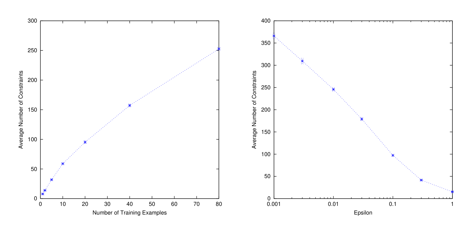{width=100%}

Figure 2 shows the number of constraints that are added to $S$ before convergence. The graph on the left-hand side shows the scaling with the number of training examples. As predicted by Theorem 18, the number of constraints is low. It appears to grow sub-linearly with the number of examples. The graph on the right-hand side shows how the number of constraints in the final $S$ changes with $\log(\varepsilon)$. The observed scaling appears to be better than suggested by the upper bound in Theorem 18. A good value for $\varepsilon$ is 0.1. We observed that larger values lead to worse prediction accuracy, while smaller values decrease efficiency while not providing further benefit.

: Table 5: Results for learning a weighted context-free grammar on the Penn Treebank.

\begin{tabular}{|l|c|c|c|c|c|c|c|c|c|c|c|c|}
\hline
 & \multicolumn{4}{c|}{Train} & \multicolumn{4}{c|}{Test} & \multicolumn{4}{c|}{Training Efficiency} \\
Method & Acc & Prec & Rec & $F_1$ & Acc & Prec & Rec & $F_1$ & CPU-h & \%SVM & Iter & Const \\
\hline
PCFG & 61.4 & 92.4 & 88.5 & 90.4 & 55.2 & 86.8 & 85.2 & 86.0 & 0 & N/A & N/A & N/A \\
$\text{SVM}_2$ & 66.3 & 92.8 & 91.2 & 92.0 & 58.9 & 85.3 & 87.2 & 86.2 & 1.2 & 81.6 & 17 & 7494 \\
$\text{SVM}_2^{\Delta s}$ & 62.2 & 93.9 & 90.4 & 92.1 & 58.9 & 88.9 & 88.1 & 88.5 & 3.4 & 10.5 & 12 & 8043 \\
$\text{SVM}_2^{\Delta m}$ & 63.5 & 93.9 & 90.8 & 92.3 & 58.3 & 88.7 & 88.1 & 88.4 & 3.5 & 18.0 & 16 & 7117 \\
\hline
\end{tabular}

5.4 Weighted Context-Free Grammars

We test the feasibility of our approach for learning a weighted context-free grammar (see Figure 1) on a subset of the Penn Treebank Wall Street Journal corpus. We consider the 4098 sentences of length at most 10 from sections F2-21 as the training set, and the 163 sentences of length at most 10 from F22 as the test set. Following the setup in Johnson (1998), we start based on the part-of-speech tags and learn a weighted grammar consisting of all rules that occur in the training data. To solve the argmax in line 6 of the algorithm, we use a modified version of the CKY parser of Mark Johnson.[^3]

[^3]: This software is available at http://www.cog.brown.edu/~mj/Software.htm.

The results are given in Table 5. They show micro-averaged precision, recall, and $F_1$ for the training and the test set. The first line shows the performance of the generative PCFG model using the maximum likelihood estimate (MLE) as computed by Johnson's implementation. The second line show the $\text{SVM}_2$ with zero-one loss, while the following lines give the results for the $F_1$-loss $\Delta(\mathbf{y}_i, \mathbf{y}) = (1 - F_1(\mathbf{y}_i, \mathbf{y}))$ using $\text{SVM}_2^{\Delta s}$ and $\text{SVM}_2^{\Delta m}$. All results are for $C = 1$ and $\varepsilon = 0.01$. All values of $C$ between $10^{-1}$ to $10^2$ gave comparable prediction performance. While the zero-one loss—which is also implicitly used in Perceptrons (Collins and Duffy, 2002a; Collins, 2002)—achieves better accuracy (i.e. predicting the complete tree correctly), the $F_1$-score is only marginally better compared to the PCFG model. However, optimizing the SVM for the $F_1$-loss gives substantially better $F_1$-scores, outperforming the PCFG substantially. The difference is significant according to a McNemar test on the $F_1$-scores. We conjecture that we can achieve further gains by incorporating more complex features into the grammar, which would be impossible or at best awkward to use in a generative PCFG model. Note that our approach can handle arbitrary models (e.g. with kernels and overlapping features) for which the argmax in line 6 can be computed. Experiments with such complex features were independently conducted by Taskar et al. (2004b) based on the algorithm in Taskar et al. (2004a). While their algorithm cannot optimize F1-score as the training loss, they report substantial gains from the use of complex features.

In terms of training time, Table 5 shows that the total number of constraints added to the working set is small. It is roughly twice the number of training examples in all cases. While the training is faster for the zero-one loss, the time for solving the QPs remains roughly comparable. The re-scaling formulations lose time mostly on the argmax in line 6 of the algorithm. This might be sped up, since we were using a rather naive algorithm in the experiments.

6. Conclusions

Section Summary: The authors introduce a maximum-margin method for learning to predict complex outputs such as structured objects or multiple interdependent variables, by modeling the task as a kernelized linear function over combined input-output features. This framework applies to problems including natural language parsing, sequence labeling, and multilabel classification. They further present a practical algorithm with proven polynomial convergence for many cases, demonstrate its effectiveness through experiments that often surpass conventional generative models, and note its flexibility to optimize custom loss functions and capture richer dependencies via kernels.

We presented a maximum-margin approach to learning functional dependencies for complex output spaces. In particular, we considered cases where the prediction is a structured object or where the prediction consists of multiple dependent variables. The key idea is to model the problem as a (kernelized) linear discriminant function over a joint feature space of inputs and outputs. We demonstrated that our approach is very general, covering problems from natural language parsing and label sequence learning to multilabel classification and classification with output features.

While the resulting learning problem can be exponential in size, we presented an algorithm for which we prove polynomial convergence for a large class of problems. We also evaluated the algorithm empirically on a broad range of applications. The experiments show that the algorithm is feasible in practice and that it produces promising results in comparison to conventional generative models. A key advantage of the algorithm is the flexibility to include different loss functions, making it possible to directly optimize the desired performance criterion. Furthermore, the ability to include kernels opens the opportunity to learn more complex dependencies compared to conventional, mostly linear models.

References

Section Summary: This section provides a bibliography of roughly three dozen academic papers and books cited throughout the document. The entries center on machine learning methods for handling structured data, such as support vector machines, sequence models, and ranking algorithms, along with their use in natural language processing and related optimization techniques. Most references come from conferences and journals in computer science from the late 1990s to the mid-2000s.

Y. Altun, I. Tsochantaridis, and T. Hofmann. Hidden Markov support vector machines. In Proceedings of the Twentieth International Conference on Machine Learning, 2003.

L. Cai and T. Hofmann. Hierarchical document categorization with support vector machines. In Proceedings of the ACM Thirteenth Conference on Information and Knowledge Management, 2004.

W. Cohen, R. Shapire, and Y. Singer. Learning to order things. Journal of Artificial Intelligence Research, 10:243–270, 1999.

M. Collins. Discriminative reranking for natural language parsing. In Proceedings of the Seventieth International Conference on Machine Learning, 2000.

M. Collins. Discriminative training methods for hidden Markov models: theory and experiments with perceptron algorithms. In Proceedings of the Conference on Empirical Methods in Natural Language Processing, 2002.

M. Collins and N. Duffy. Convolution kernels for natural language. In Advances in Neural Information Processing Systems 14, pages 625–632, 2002a.

M. Collins and N. Duffy. New ranking algorithms for parsing and tagging: kernels over discrete structures, and the voted perceptron. In Proceedings of the Fortieth Annual Meeting of the Association for Computational Linguistics, 2002b.

K. Crammer and Y. Singer. On the algorithmic implementation of multi-class kernel-based vector machines. Machine Learning Research, 2:265–292, 2001.

K. Crammer and Y. Singer. Pranking with ranking. In Advances in Neural Information Processing Systems 14, 2002.

R. Durbin, S. Eddy, A. Krogh, and G. Mitchison. Biological Sequence Analysis. Cambridge University Press, 1998.

G. D. Forney Jr. The Viterbi algorithm. Proceedings of the IEEE, 61:268–278, 1973.

M. Grötschel, L. Lovàtz, and A. Schrijver. The ellipsoid method and its consequences in combinatorial optimization. Combinatorica, 1(2):169–197, 1981.

S. Har-Peled, D. Roth, and D. Zimak. Constraint classification for multiclass classification and ranking. In Advances in Neural Information Processing Systems 14, 2002.

R. Herbrich, T. Graepel, and K. Obermayer. Large margin rank boundaries for ordinal regression. In Advances in Large Margin Classifiers. MIT Press, Cambridge, MA, 2000.

T. Hofmann, I. Tsochantaridis, and Y. Altun. Learning over structured output spaces via joint kernel functions. In Proceedings of the Sixth Kernel Workshop, 2002.

T. Joachims. Optimizing search engines using clickthrough data. In Proceedings of the ACM Conference on Knowledge Discovery and Data Mining, 2002.

T. Joachims. Learning to align sequences: A maximum-margin approach. Technical report, Cornell University, 2003.

T. Joachims. A support vector method for multivariate performance measures. In Proceedings of the Twenty-Second International Conference on Machine Learning, 2005.

M. Johnson. PCFG models of linguistic tree representations. Computational Linguistics, 24(4):613–632, 1998.

N. Karmarkar. A new polynomial-time algorithm for linear programming. Combinatorica, 4(4):373–396, 1984.

J. E. Kelley. The cutting-plane method for solving convex programs. Journal of the Society for Industrial Applied Mathematics, 8:703–712, 1960.

J. Lafferty, A. McCallum, and F. Pereira. Conditional random fields: Probabilistic models for segmenting and labeling sequence data. In Proceedings of the Eighteenth International Conference on Machine Learning, pages 282–289, 2001.

C. D. Manning and H. Schuetze. Foundations of Statistical Natural Language Processing. MIT Press, Cambridge, MA, 1999.

E. Ristad and P. Yianilos. Learning string edit distance. In Proceedings of the Seventeenth International Conference on Machine Learning, pages 287–295, 1997.

R. E. Schapire and Y. Singer. Boostexter: A boosting-based system for text categorization. Machine Learning, 39(2-3):135–168, 2000.

R. Schwarz and Y. L. Chow. The n-best algorithm: An efficient and exact procedure for finding the n most likely hypotheses. In Proceedings of the IEEE International Conference on Acoustics, Speech and Signal Processing, pages 81–84, 1990.

A. Smola and T. Hofmann. Exponential families for generative and discriminative estimation. Technical report, 2003.

B. Taskar, C. Guestrin, and D. Koller. Max-margin Markov networks. In Advances in Neural Information Processing Systems 16, 2004a.

B. Taskar, D. Klein, M. Collins, D. Koller, and C. Manning. Max-Margin parsing. In Proceedings of the Conference on Empirical Methods in Natural Language Processing, 2004b.

I. Tsochantaridis, T. Hofmann, T. Joachims, and Y. Altun. Support vector machine learning for interdependent and structured output spaces. In Proceedings of the Twenty-First International Conference on Machine Learning, 2004.

V. Vapnik. Statistical Learning Theory. Wiley and Sons Inc., New York, 1998.

J. Weston, O. Chapelle, A. Elisseeff, B. Schölkopf, and V. Vapnik. Kernel dependency estimation. In Advances in Neural Information Processing Systems 15, 2003.

J. Weston and C. Watkins. Multi-class support vector machines. Technical Report CSD-TR-98-04, Department of Computer Science, Royal Holloway, University of London, 1998.

D. H. Younger. Recognition and parsing of context-free languages in time $n^3$. Information and Control, 2(10):189–208, 1967.