Executive Summary: In the mid-20th century, scientists grappled with fundamental questions about the brain's ability to sense, store, and use information for recognition, learning, and decision-making. While sensory detection was somewhat understood, how the brain remembers experiences and applies them to new situations remained speculative. Two competing ideas dominated: one viewed memory as precise, coded replicas of stimuli, like snapshots in a computer; the other saw it as flexible connections between brain cells, forming pathways that link similar inputs to specific outputs without exact reconstructions. This debate was crucial amid rising interest in artificial intelligence and computing, as it promised insights into building machines that mimic human cognition, potentially revolutionizing fields like automation and psychology.

This document introduces the Perceptron, a theoretical model of a brain-like system designed to explore information storage and behavioral influence through probabilistic connections rather than rigid logic. Rosenblatt aimed to demonstrate how random neural networks could achieve learning and pattern recognition, drawing from biological inspirations like cell assemblies while avoiding the pitfalls of overly deterministic models.

The approach involved creating a simplified neural network architecture with three layers: sensory units that detect inputs (like light patterns on a retina), association units that process and connect signals randomly, and response units that output actions or decisions. Connections between units could strengthen or weaken based on activity and reinforcement, mimicking learning without predefined wiring. The model assumed modifiable cell strengths (called "value") and used probability theory to analyze performance, focusing on key parameters such as the number of connections per cell, activation thresholds, and system size. Analysis covered hypothetical experiments in two environments: a random "ideal" setup with unrelated stimuli, and a structured "differentiated" one with distinct classes (e.g., shapes like squares versus circles). Computer simulations on early machines like the IBM 704 validated the math, testing learning under repeated exposures without forcing outcomes.

The analysis revealed several core insights. First, in random environments, the Perceptron reliably associated specific stimuli with responses, achieving better-than-chance accuracy (around 50-70% initially, improving with repetitions), but performance degraded as more unrelated items were learned, and it showed no ability to generalize to new examples. Second, in structured settings with similar stimuli grouped by class, the system excelled: it discriminated classes with over 90% accuracy after thousands of trials, approaching near-perfect performance as the number of association cells grew (e.g., from 1,000 to 10,000 units boosted success rates by 20-30%). Generalization matched exact recall, meaning unseen but similar stimuli triggered correct responses at the same high rate. Third, enhancements like binary coding (breaking responses into independent "yes/no" features, such as "curved" or "straight") and contour-detecting input layers improved efficiency, allowing distinction of dozens of classes with fewer resources. Fourth, adding positive and negative reinforcement enabled trial-and-error learning, where errors refined connections faster than rewards alone. Finally, the system's memory was distributed across cells, making it resilient—removing some units caused only minor, broad declines rather than total failure for specific tasks.

These findings matter because they offer a principled alternative to earlier brain models, which often relied on unrealistic precision or failed biological tests like flexibility and fault tolerance. The Perceptron shows how random, adaptable networks can handle perceptual tasks like recognizing shapes or associating sounds with visuals, impacting costs and timelines in AI development by suggesting simple hardware could achieve robust intelligence. Unlike prior theories based on observed behavior (prone to circular reasoning), this one predicts outcomes from measurable physical traits, enhancing verifiability and generality across species or machines. It challenges coded-memory ideas by proving connections alone suffice for learning without stimulus reconstruction, potentially reshaping psychology and engineering. Deviations from expectations, like poor performance in random settings, highlight the need for environmental structure in real-world applications, such as training AI for consistent data.

Next steps include building physical Perceptrons for empirical testing, starting with basic photo-sensitive prototypes to validate discrimination tasks. Simulations should expand to multi-sensory inputs (e.g., combining vision and sound) and temporal sequences (e.g., motion detection) to broaden capabilities. For decision-makers, prioritize binary response designs for scalability, trading slight complexity for 2-3x efficiency in class recognition. If aiming for advanced uses like robotics, pilot integrations with feedback loops for sequential behaviors, but delay until abstractions like spatial relationships are addressed through layered extensions.

Key limitations include simplifications, such as all-or-nothing cell firing and no feedback until the final layer, which may not fully match real neurons; data gaps persist on exact biological correlates for "value" changes. The model struggles with abstract judgments, like comparing stimuli rather than identifying them directly, limiting it to concrete tasks. Confidence is strong in the mathematical predictions for basic learning (supported by simulations), but moderate for biological applicability—readers should view it as a promising framework needing lab validation before broad adoption.

The perceptron: A probabilistic model for information storage and organization in the brain[^1]

Frank Rosenblatt
Cornell Aeronautical Laboratory

[^1]: The development of this theory has been carried out at the Cornell Aeronautical Laboratory, Inc., under the sponsorship of the Office of Naval Research, Contract Nonr 2381(00). This article is primarily an adaptation of material reported in Ref. 15, which constitutes the first full report on the program.

If we are eventually to understand the capability of higher organisms for perceptual recognition, generalization, recall, and thinking, we must first have answers to three fundamental questions:

1. How is information about the physical world sensed, or detected, by the biological system?
2. In what form is information stored, or remembered?
3. How does information contained in storage, or in memory, influence recognition and behavior?

The first of these questions is in the province of sensory physiology, and is the only one for which appreciable understanding has been achieved. This article will be concerned primarily with the second and third questions, which are still subject to a vast amount of speculation, and where the few relevant facts currently supplied by neurophysiology have not yet been integrated into an acceptable theory.

With regard to the second question, two alternative positions have been maintained. The first suggests that storage of sensory information is in the form of coded representations or images, with some sort of one-to-one mapping between the sensory stimulus and the stored pattern. According to this hypothesis, if one understood the code or "wiring diagram" of the nervous system, one should, in principle, be able to discover exactly what an organism remembers by reconstructing the original sensory patterns from the "memory traces" which they have left, much as we might develop a photographic negative, or translate the pattern of electrical charges in the "memory" of a digital computer. This hypothesis is appealing in its simplicity and ready intelligibility, and a large family of theoretical brain models has been developed around the idea of a coded, representational memory (2, 3, 9, 14). The alternative approach, which stems from the tradition of British empiricism, hazards the guess that the images of stimuli may never really be recorded at all, and that the central nervous system simply acts as an intricate switching network, where retention takes the form of new connections, or pathways, between centers of activity. In many of the more recent developments of this position (Hebb's "cell assembly," and Hull's "cortical anticipatory goal response," for example) the "responses" which are associated to stimuli may be entirely contained within the CNS itself. In this case the response represents an "idea" rather than an action. The important feature of this approach is that there is never any simple mapping of the stimulus into memory, according to some code which would permit its later reconstruction. Whatever information is retained must somehow be stored as a preference for a particular response; i.e., the information is contained in connections or associations rather than topographic representations. (The term response, for the remainder of this presentation, should be understood to mean any distinguishable state of the organism, which may or may not involve externally detectable muscular activity. The activation of some nucleus of cells in the central nervous system, for example, can constitute a response, according to this definition.)

Corresponding to these two positions on the method of information retention, there exist two hypotheses with regard to the third question, the manner in which stored information exerts its influence on current activity. The "coded memory theorists" are forced to conclude that recognition of any stimulus involves the matching or systematic comparison of the contents of storage with incoming sensory patterns, in order to determine whether the current stimulus has been seen before, and to determine the appropriate response from the organism. The theorists in the empiricist tradition, on the other hand, have essentially combined the answer to the third question with their answer to the second: since the stored information takes the form of new connections, or transmission channels in the nervous system (or the creation of conditions which are functionally equivalent to new connections), it follows that the new stimuli will make use of these new pathways which have been created, automatically activating the appropriate response without requiring any separate process for their recognition or identification.

The theory to be presented here takes the empiricist, or "connectionist" position with regard to these questions. The theory has been developed for a hypothetical nervous system, or machine, called a perceptron. The perceptron is designed to illustrate some of the fundamental properties of intelligent systems in general, without becoming too deeply enmeshed in the special, and frequently unknown, conditions which hold for particular biological organisms. The analogy between the perceptron and biological systems should be readily apparent to the reader.

During the last few decades, the development of symbolic logic, digital computers, and switching theory has impressed many theorists with the functional similarity between a neuron and the simple on-off units of which computers are constructed, and has provided the analytical methods necessary for representing highly complex logical functions in terms of such elements. The result has been a profusion of brain models which amount simply to logical contrivances for performing particular algorithms (representing "recall," stimulus comparison, transformation, and various kinds of analysis) in response to sequences of stimuli—e.g., Rashevsky (14), McCulloch (10), McCulloch & Pitts (11), Culbertson (2), Kleene (8), and Minsky (13). A relatively small number of theorists, like Ashby (1) and von Neumann (17, 18), have been concerned with the problems of how an imperfect neural network, containing many random connections, can be made to perform reliably those functions which might be represented by idealized wiring diagrams. Unfortunately, the language of symbolic logic and Boolean algebra is less well suited for such investigations. The need for a suitable language for the mathematical analysis of events in systems where only the gross organization can be characterized, and the precise structure is unknown, has led the author to formulate the current model in terms of probability theory rather than symbolic logic.

The theorists referred to above were chiefly concerned with the question of how such functions as perception and recall might be achieved by a deterministic physical system of any sort, rather than how this is actually done by the brain. The models which have been produced all fail in some important respects (absence of equipotentiality, lack of neuroeconomy, excessive specificity of connections and synchronization requirements, unrealistic specificity of stimuli sufficient for cell firing, postulation of variables or functional features with no known neurological correlates, etc.) to correspond to a biological system. The proponents of this line of approach have maintained that, once it has been shown how a physical system of any variety might be made to perceive and recognize stimuli, or perform other brainlike functions, it would require only a refinement or modification of existing principles to understand the working of a more realistic nervous system, and to eliminate the shortcomings mentioned above. The writer takes the position, on the other hand, that these shortcomings are such that a mere refinement or improvement of the principles already suggested can never account for biological intelligence; a difference in principle is clearly indicated. The theory of statistical separability (Cf. 15), which is to be summarized here, appears to offer a solution in principle to all of these difficulties.

Those theorists—Hebb (7), Milner (12), Eccles (4), Hayek (6)—who have been more directly concerned with the biological nervous system and its activity in a natural environment, rather than with formally analogous machines, have generally been less exact in their formulations and far from rigorous in their analysis, so that it is frequently hard to assess whether or not the systems that they describe could actually work in a realistic nervous system, and what the necessary and sufficient conditions might be. Here again, the lack of an analytic language comparable in proficiency to the Boolean algebra of the network analysts has been one of the main obstacles. The contributions of this group should perhaps be considered as suggestions of what to look for and investigate, rather than as finished theoretical systems in their own right. Seen from this viewpoint, the most suggestive work, from the standpoint of the following theory, is that of Hebb and Hayek.

The position, elaborated by Hebb (7), Hayek (6), Uttley (16), and Ashby (1), in particular, upon which the theory of the perceptron is based, can be summarized by the following assumptions:

1. The physical connections of the nervous system which are involved in learning and recognition are not identical from one organism to another. At birth, the construction of the most important networks is largely random, subject to a minimum number of genetic constraints.
2. The original system of connected cells is capable of a certain amount of plasticity; after a period of neural activity, the probability that a stimulus applied to one set of cells will cause a response in some other set is likely to change, due to some relatively long-lasting changes in the neurons themselves.
3. Through exposure to a large sample of stimuli, those which are most "similar" (in some sense which must be defined in terms of the particular physical system) will tend to form pathways to the same sets of responding cells. Those which are markedly "dissimilar" will tend to develop connections to different sets of responding cells.
4. The application of positive and/or negative reinforcement (or stimuli which serve this function) may facilitate or hinder whatever formation of connections is currently in progress.
5. Similarity, in such a system, is represented at some level of the nervous system by a tendency of similar stimuli to activate the same sets of cells. Similarity is not a necessary attribute of particular formal or geometrical classes of stimuli, but depends on the physical organization of the perceiving system, an organization which evolves through interaction with a given environment. The structure of the system, as well as the ecology of the stimulus-environment, will affect, and will largely determine, the classes of "things" into which the perceptual world is divided.

THE ORGANIZATION OF A PERCEPTRON

Section Summary: A perceptron is a layered network designed to recognize patterns such as visual images. Light hits a grid of simple sensors that fire when sufficiently stimulated, and their signals travel through one or more stages of connecting cells whose wiring is largely random. The final layer contains response units that can reinforce their own active inputs or suppress competing ones, allowing the system to strengthen the pathways that lead to correct classifications.

The organization of a typical photoperceptron (a perceptron responding to optical patterns as stimuli) is shown in Fig. 1. The rules of its organization are as follows:

1. Stimuli impinge on a retina of sensory units (S-points), which are assumed to respond on an all-or-nothing basis, in some models, or with a pulse amplitude or frequency proportional to the stimulus intensity, in other models. In the models considered here, an all-or-nothing response will be assumed.
2. Impulses are transmitted to a set of association cells (A-units) in a "projection area" ($A_I$). This projection area may be omitted in some models, where the retina is connected directly to the association area ($A_{II}$).

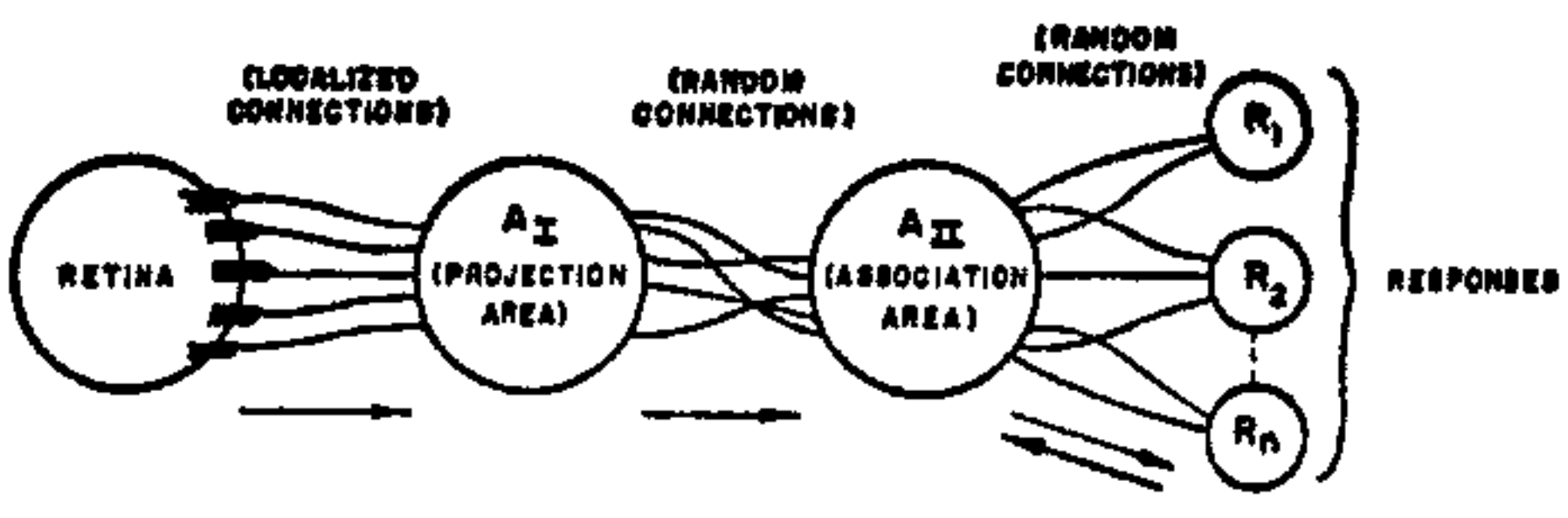
The cells in the projection area each receive a number of connections from the sensory points. The set of S-points transmitting impulses to a particular A-unit will be called the origin points of that A-unit. These origin points may be either excitatory or inhibitory in their effect on the A-unit. If the algebraic sum of excitatory and inhibitory impulse intensities is equal to or greater than the threshold ($\theta$) of the A-unit, then the A-unit fires, again on an all-or-nothing basis (or, in some models, which will not be considered here, with a frequency which depends on the net value of the impulses received). The origin points of the A-units in the projection area tend to be clustered or focalized, about some central point, corresponding to each A-unit. The number of origin points falls off exponentially as the retinal distance from the central point for the A-unit in question increases. (Such a distribution seems to be supported by physiological evidence, and serves an important functional purpose in contour detection.)

3. Between the projection area and the association area ($A_{II}$), connections are assumed to be random. That is, each A-unit in the $A_{II}$ set receives some number of fibers from origin points in the $A_I$ set, but these origin points are scattered at random throughout the projection area. Apart from their connection distribution, the $A_{II}$ units are identical with the $A_I$ units, and respond under similar conditions.
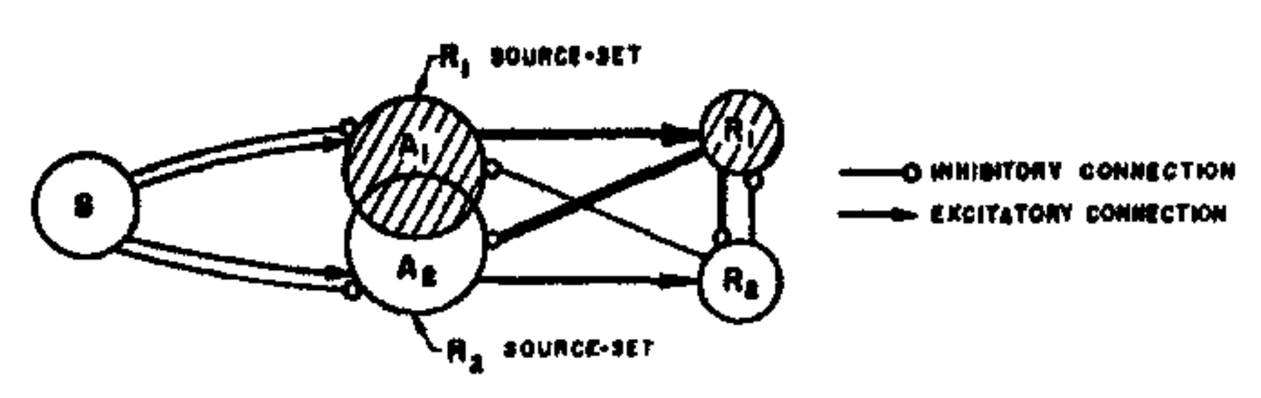
4. The "responses," $R_1, R_2, \dots, R_n$ are cells (or sets of cells) which respond in much the same fashion as the A-units. Each response has a typically large number of origin points located at random in the $A_{II}$ set. The set of A-units transmitting impulses to a particular response will be called the source-set for that response. (The source-set of a response is identical to its set of origin points in the A-system.) The arrows in Fig. 1 indicate the direction of transmission through the network. Note that up to $A_{II}$ all connections are forward, and there is no feedback. When we come to the last set of connections, between $A_{II}$ and the R-units, connections are established in both directions. The rule governing feedback connections, in most models of the perceptron, can be either of the following alternatives: (a) Each response has excitatory feedback connections to the cells in its own source-set, or (b) Each response has inhibitory feedback connections to the complement of its own source-set (i.e., it tends to prohibit activity in any association cells which do not transmit to it).

The first of these rules seems more plausible anatomically, since the R-units might be located in the same cortical area as their respective source-sets, making mutual excitation between the R-units and the A-units of the appropriate source-set highly probable. The alternative rule ($b$) leads to a more readily analyzed system, however, and will therefore be assumed for most of the systems to be evaluated here.

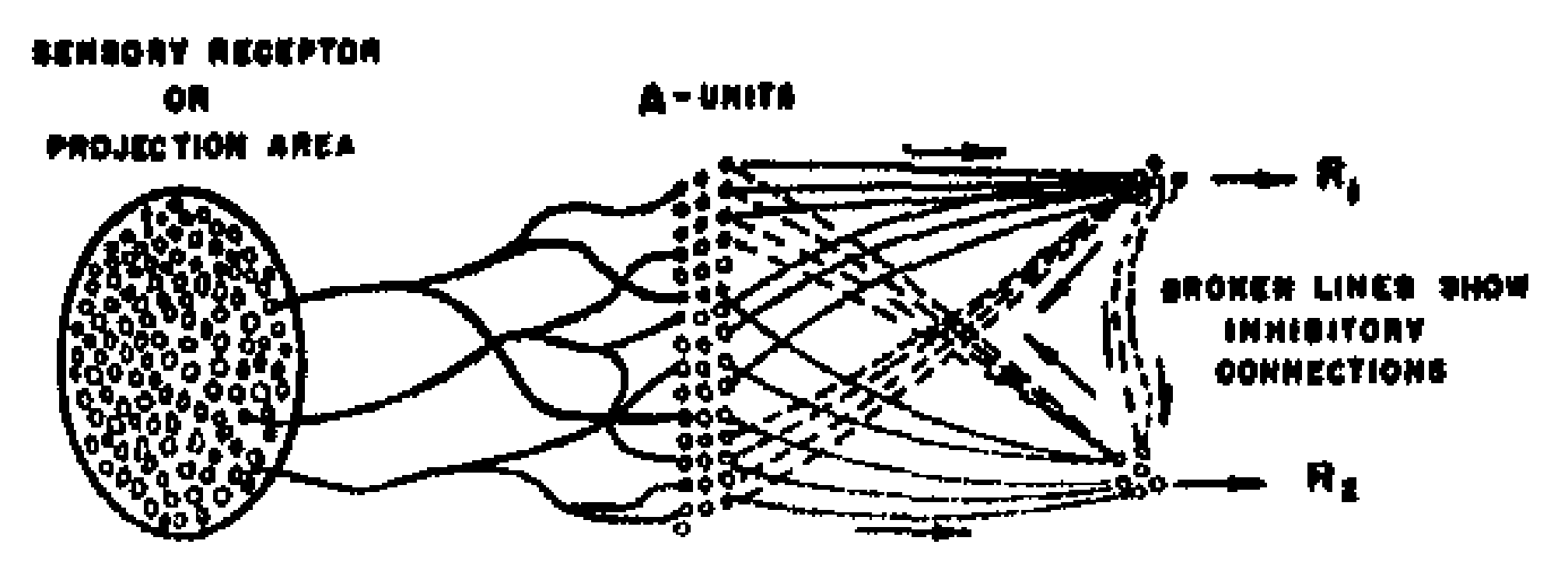
Figure 2 shows the organization of a simplified perceptron, which affords a convenient entry into the theory of statistical separability. After the theory has been developed for this simplified model, we will be in a better position to discuss the advantages of the system in Fig. 1. The feedback connections shown in Fig. 2 are inhibitory, and go to the complement of the source-set for the response from which they originate; consequently, this system is organized according to Rule $b$, above. The system shown here has only three stages, the first association stage having been eliminated. Each A-unit has a set of randomly located origin points in the retina. Such a system will form similarity concepts on the basis of coincident areas of stimuli, rather than by the similarity of contours or outlines. While such a system is at a disadvantage in many discrimination experiments, its capability is still quite impressive, as will be demonstrated presently. The system shown in Fig. 2 has only two responses, but there is clearly no limit on the number that might be included.

The responses in a system organized in this fashion are mutually exclusive. If $R_1$ occurs, it will tend to inhibit $R_2$, and will also inhibit the source-set for $R_2$. Likewise, if $R_2$ should occur, it will tend to inhibit $R_1$. If the total impulse received from all the A-units in one source-set is stronger or more frequent than the impulse received by the alternative (antagonistic) response, then the first response will tend to gain an advantage over the other, and will be the one which occurs. If such a system is to be capable of learning, then it must be possible to modify the A-units or their connections in such a way that stimuli of one class will tend to evoke a stronger impulse in the $R_1$ source-set than in the $R_2$ source-set, while stimuli of another (dissimilar) class will tend to evoke a stronger impulse in the $R_2$ source-set than in the $R_1$ source-set.

It will be assumed that the impulses delivered by each A-unit can be characterized by a value, $V$, which may be an amplitude, frequency, latency, or probability of completing transmission. If an A-unit has a high value, then all of its output impulses are considered to be more effective, more potent, or more likely to arrive at their endbulbs than impulses from an A-unit with a lower value. The value of an A-unit is considered to be a fairly stable characteristic, probably depending on the metabolic condition of the cell and the cell membrane, but it is not absolutely constant. It is assumed that, in general, periods of activity tend to increase a cell's value, while the value may decay (in some models) with inactivity. The most interesting models are those in which cells are assumed to compete for metabolic materials, the more active cells gaining at the expense of the less active cells. In such a system, if there is no activity, all cells will tend to remain in a relatively constant condition, and (regardless of activity) the net value of the system, taken in its entirety, will remain constant at all times. Three types of systems, which differ in their value dynamics, have been investigated quantitatively. Their principal logical features are compared in Table 1. In the alpha system, an active cell simply gains an increment of value for every impulse, and holds this gain indefinitely. In the beta system, each source-set is allowed a certain constant rate of gain, the increments being apportioned among the cells of the source-set in proportion to their activity. In the gamma system, active cells gain in value at the expense of the inactive cells of their source-set, so that the total value of a source-set is always constant.

: Table 1: Comparison of Logical Characteristics of $\alpha$, $\beta$, and $\gamma$ Systems.

\begin{tabular}{l|c|c|c}
\hline
 & \begin{tabular}[c]{@{}c@{}}$\alpha$-System\\ (Uncompensated\\ Gain System)\end{tabular} & \begin{tabular}[c]{@{}c@{}}$\beta$-System\\ (Constant Feed\\ System)\end{tabular} & \begin{tabular}[c]{@{}c@{}}$\gamma$-System\\ (Parasitic Gain\\ System)\end{tabular} \\ \hline
Total value-gain of source set per reinforcement & $N_{a_r}$ & $K$ & 0 \\ \hline
$\Delta V$ for A-units active for 1 unit of time & +1 & $K/N_{a_r}$ & +1 \\ \hline
\begin{tabular}[c]{@{}l@{}}$\Delta V$ for inactive A-units outside of domi-\\ nant set\end{tabular} & 0 & $K/N_{A_r}$ & 0 \\ \hline
$\Delta V$ for inactive A-units of dominant set & 0 & 0 & $\frac{-N_{a_r}}{N_{A_r} - N_{a_r}}$ \\ \hline
Mean value of A-system & \begin{tabular}[c]{@{}l@{}}Increases with number\\ of reinforcements\end{tabular} & \begin{tabular}[c]{@{}l@{}}Increases with\\ time\end{tabular} & Constant \\ \hline
\begin{tabular}[c]{@{}l@{}}Difference between mean values of\\ source-sets\end{tabular} & \begin{tabular}[c]{@{}l@{}}Proportional to differ-\\ ences of reinforce-\\ ment frequency\\ ($n_{sr_1} - n_{sr_2}$)\end{tabular} & 0 & 0 \\ \hline
\end{tabular}

Note: In the $\beta$ and $\gamma$ systems, the total value-change for any A-unit will be the sum of the $\Delta V

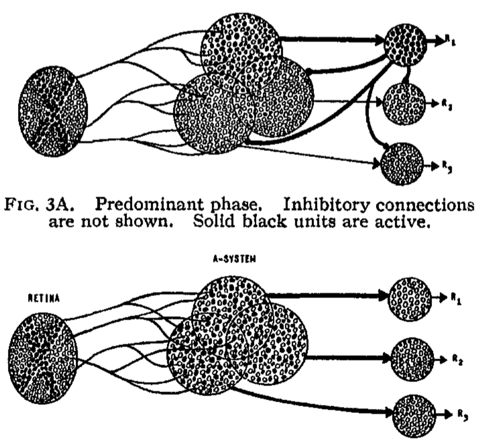
#39;s for all source-sets of which it is a member. $N_{a_r} = $ Number of active units in source-set $N_{A_r} = $ Total number of units in source-set $n_{sr_j} = $ Number of stimuli associated to response $r_j$ $K = $ Arbitrary constant

For purposes of analysis, it is convenient to distinguish two phases in the response of the system to a stimulus (Fig. 3). In the predominant phase, some proportion of A-units (represented by solid dots in the figure) responds to the stimulus, but the R-units are still inactive. This phase is transient, and quickly gives way to the postdominant phase, in which one of the responses becomes active, inhibiting activity in the complement of its own source-set, and thus preventing the occurrence of any alternative response. The response which happens to become dominant is initially random, but if the A-units are reinforced (i.e., if the active units are allowed to gain in value), then when the same stimulus is presented again at a later time, the same response will have a stronger tendency to recur, and learning can be said to have taken place.

ANALYSIS OF THE PREDOMINANT PHASE

Section Summary: The section analyzes fixed-threshold perceptrons, where A-units activate only when their net excitatory input reaches a set threshold, unlike models with graded responses. Two key probabilities—Pa, the fraction of A-units that fire for a given stimulus, and Pc, the chance that an A-unit activated by one stimulus will also fire for a second stimulus—dominate predictions of learning performance. These values depend on retinal size, the balance of excitatory and inhibitory connections, the threshold level, and the degree of overlap between stimuli; higher thresholds or more inhibition sharply reduce both, while Pc remains useful for distinguishing patterns even when stimuli share no points.

The perceptrons considered here will always assume a fixed threshold, $\theta$, for the activation of the A-units. Such a system will be called a fixed-threshold model, in contrast to a continuous transducer model, where the response of the A-unit is some continuous function of the impinging stimulus energy.

In order to predict the learning curves of a fixed-threshold perceptron, two variables have been found to be of primary importance. They are defined as follows:

$P_a =$ the expected proportion of A-units activated by a stimulus of a given size, $P_c =$ the conditional probability that an A-unit which responds to a given stimulus, $S_1$, will also respond to another given stimulus, $S_2$.

It can be shown (Rosenblatt, 15) that as the size of the retina is increased, the number of S-points ($N_s$) quickly ceases to be a significant parameter, and the values of $P_a$ and $P_c$ approach the value that they would have for a retina with infinitely many points. For a large retina, therefore, the equations are as follows:

$ P_a = \sum_{e = \theta}^x \sum_{i = \theta}^{\min(y, e - \theta)} P(e, i)\tag{1} $

where

$ P(e, i) = \binom{x}{e} R^e(1 - R)^{x-e} \times \binom{y}{i} R^i(1 - R)^{y-i} $

and $R =$ proportion of S-points activated by the stimulus $x =$ number of excitatory connections to each A-unit $y =$ number of inhibitory connections to each A-unit $\theta =$ threshold of A-units.

(The quantities $e$ and $i$ are the excitatory and inhibitory components of the excitation received by the A-unit from the stimulus. If the algebraic sum $a = e + i$ is equal to or greater than $\theta$, the A-unit is assumed to respond.)

$ P_c = \frac{1}{P_a} \sum_{e=0}^x \sum_{i=0}^y \sum_{l_e=0}^e \sum_{l_i=0}^i \sum_{g_e=0}^{x-e} \sum_{g_i=0}^{y-i} P(e, i, l_e, l_i, g_e, g_i)\tag{2} $

($e - i - l_e + l_i + g_e - g_i \geq \theta$)

where

$ \begin{aligned} P(e, i, l_e, l_i, g_e, g_i) = & \binom{x}{e} R^e(1 - R)^{x-e} \ & \times \binom{y}{i} R^i(1 - R)^{y-i} \ & \times \binom{e}{l_e} L^{l_e}(1 - L)^{e-l_e} \ & \times \binom{i}{l_i} L^{l_i}(1 - L)^{i-l_i} \ & \times \binom{x-e}{g_e} G^{g_e}(1 - G)^{x-e-g_e} \ & \times \binom{y-i}{g_i} G^{g_i}(1 - G)^{y-i-g_i} \end{aligned} $

and $L =$ proportion of the S-points illuminated by the first stimulus, $S_1$, which are not illuminated by $S_2$ $G =$ proportion of the residual S-set (left over from the first stimulus) which is included in the second stimulus ($S_2$).

The quantities $R, L,$ and $G$ specify the two stimuli and their retinal overlap. $l_e$ and $l_i$ are, respectively, the numbers of excitatory and inhibitory origin points "lost" by the A-unit when stimulus $S_1$ is replaced by $S_2$; $g_e$ and $g_i$ are the numbers of excitatory and inhibitory origin points "gained" when stimulus $S_1$ is replaced by $S_2$. The summations in Equation 2 are between the limits indicated, subject to the side condition $e - i - l_e + l_i + g_e - g_i \geq \theta$.

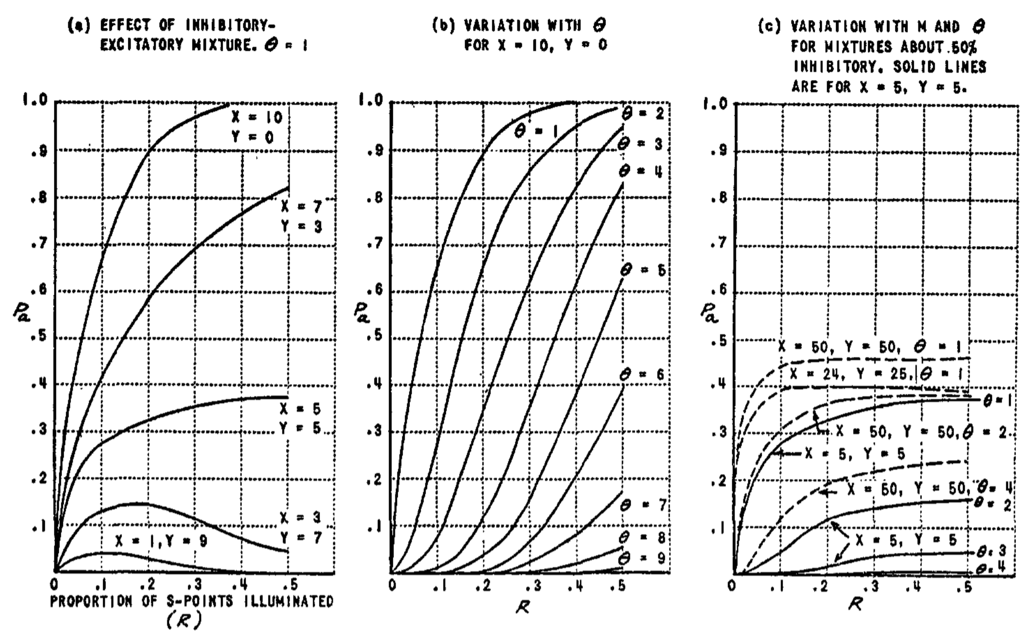
Some of the most important characteristics of $P_a$ are illustrated in Fig. 4, which shows $P_a$ as a function of the retinal area illuminated ($R$). Note that $P_a$ can be reduced in magnitude by either increasing the threshold, $\theta$, or by increasing the proportion of inhibitory connections ($y$). A comparison of Fig. 4b and 4c shows that if the excitation is about equal to the inhibition, the curves for $P_a$ as a function of $R$ are flattened out, so that there is little variation in $P_a$ for stimuli of different sizes. This fact is of great importance for systems which require $P_a$ to be close to an optimum value in order to perform properly.

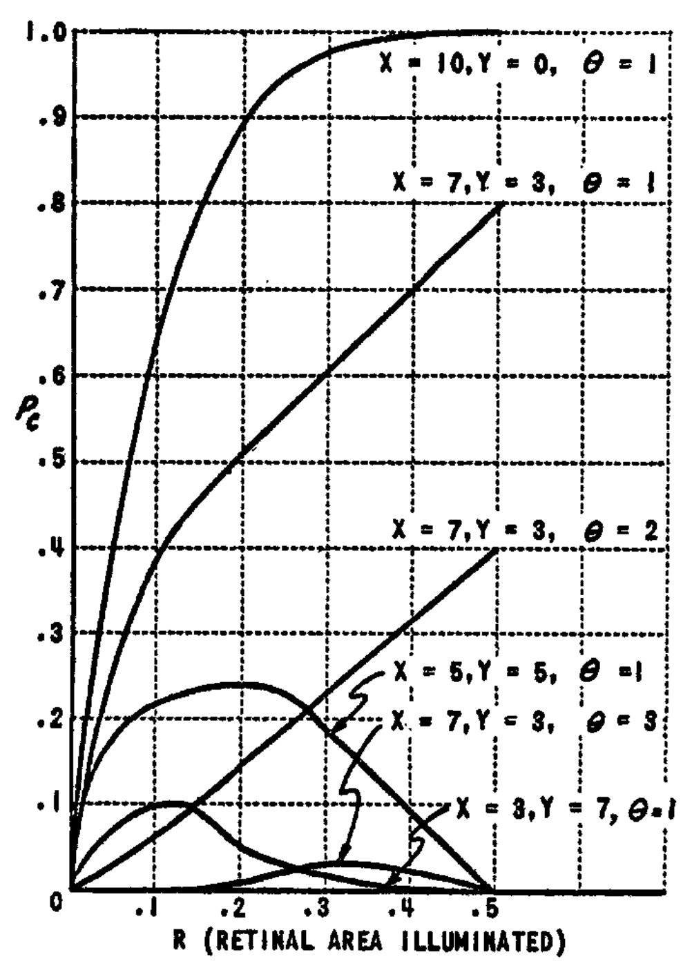
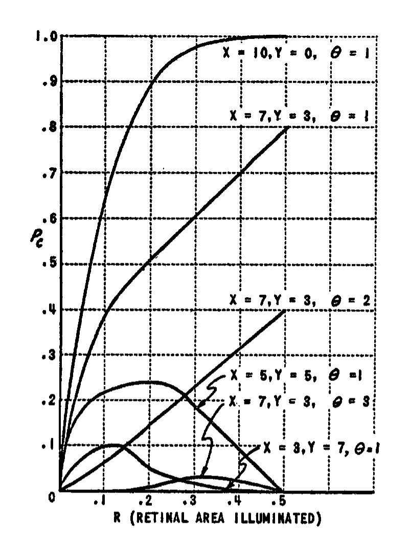
The behavior of $P_c$ is illustrated in Fig. 5 and 6. The curves in Fig. 5 can be compared with those for $P_a$ in Fig. 4. Note that as the threshold is increased, there is an even sharper reduction in the value of $P_c$ than was the case with $P_a$. $P_c$ also decreases as the proportion of inhibitory connections increases, as does $P_a$. Fig. 5, which is calculated for nonoverlapping stimuli, illustrates the fact that $P_c$ remains greater than zero even when the stimuli are completely disjunct, and illuminate no retinal points in common. In Fig. 6, the effect of varying amounts of overlap between the stimuli is shown. In all cases, the value of $P_c$ goes to unity as the stimuli approach perfect identity. For smaller stimuli (broken line curves), the value of $P_c$ is lower than for large stimuli. Similarly, the value is less for high thresholds than for low thresholds. The minimum value of $P_c$ will be equal to

$ P_{c_{\min}} = (1 - L)^x (1 - G)^y.\tag{3} $

In Fig. 6, $P_{c_{\min}}$ corresponds to the curve for $\theta = 10$. Note that under these conditions the probability that the A-unit responds to both stimuli ($P_c$) is practically zero, except for stimuli which are quite close to identity. This condition can be of considerable help in discrimination learning.

MATHEMATICAL ANALYSIS OF LEARNING IN THE PERCEPTRON

Section Summary: The section examines how perceptrons transition from widespread responses across many association units to a single dominant response, comparing systems that select based on average versus total input strength, with the former proving more robust to random variations. It outlines two evaluation methods—one measuring accurate recall of specific trained stimuli (via probability Pr) and another testing generalization to new examples from the same classes (via Pg)—both modeled by a shared approximate equation that integrates activation probabilities with a normal-curve adjustment for bias after repeated exposures. The analysis emphasizes how effective, non-overlapping units drive learning performance while common connections contribute no net advantage.

The response of the perceptron in the predominant phase, where some fraction of the A-units (scattered throughout the system) responds to the stimulus, quickly gives way to the postdominant response, in which activity is limited to a single source-set, the other sets being suppressed. Two possible systems have been studied for the determination of the "dominant" response, in the postdominant phase. In one (the mean-discriminating system, or $\mu$-system), the response whose inputs have the greatest mean value responds first, gaining a slight advantage over the others, so that it quickly becomes dominant. In the second case (the sum-discriminating system, or $\Sigma$-system), the response whose inputs have the greatest net value gains an advantage. In most cases, systems which respond to mean values have an advantage over systems which respond to sums, since the means are less influenced by random variations in $P_a$ from one source-set to another. In the case of the $\gamma$-system (see Table 1), however, the performance of the $\mu$-system and $\Sigma$-system become identical.

We have indicated that the perceptron is expected to learn, or to form associations, as a result of the changes in value that occur as a result of the activity of the association cells. In evaluating this learning, one of two types of hypothetical experiments can be considered. In the first case, the perceptron is exposed to some series of stimulus patterns (which might be presented in random positions on the retina) and is "forced" to give the desired response in each case. (This forcing of responses is assumed to be a prerogative of the experimenter. In experiments intended to evaluate trial-and-error learning, with more sophisticated perceptrons, the experimenter does not force the system to respond in the desired fashion, but merely applies positive reinforcement when the response happens to be correct, and negative reinforcement when the response is wrong.) In evaluating the learning which has taken place during this "learning series," the perceptron is assumed to be "frozen" in its current condition, no further value changes being allowed, and the same series of stimuli is presented again in precisely the same fashion, so that the stimuli fall on identical positions on the retina. The probability that the perceptron will show a bias towards the "correct" response (the one which has been previously reinforced during the learning series) in preference to any given alternative response is called $P_r$, the probability of correct choice of response between two alternatives.

In the second type of experiment, a learning series is presented exactly as before, but instead of evaluating the perceptron's performance using the same series of stimuli which were shown before, a new series is presented, in which stimuli may be drawn from the same classes that were previously experienced, but are not necessarily identical. This new test series is assumed to be composed of stimuli projected onto random retinal positions, which are chosen independently of the positions selected for the learning series. The stimuli of the test series may also differ in size or rotational position from the stimuli which were previously experienced. In this case, we are interested in the probability that the perceptron will give the correct response for the class of stimuli which is represented, regardless of whether the particular stimulus has been seen before or not. This probability is called $P_g$, the probability of correct generalization. As with $P_r$, $P_g$ is actually the probability that a bias will be found in favor of the proper response rather than any one alternative; only one pair of responses at a time is considered, and the fact that the response bias is correct in one pair does not mean that there may not be other pairs in which the bias favors the wrong response. The probability that the correct response will be preferred over all alternatives is designated $P_R$ or $P_G$.

In all cases investigated, a single general equation gives a close approximation to $P_r$ and $P_g$, if the appropriate constants are substituted. This equation is of the form:

$ P = P(N_{a_r} > 0) \cdot \Phi(Z)\tag{4} $

where

$ P(N_{a_r} > 0) = 1 - (1 - P_a)^{N_e} $

$\Phi(Z) = $ normal curve integral from $-\infty$ to $Z$

and

$ Z = \frac{c_1 n_{sr} + c_2}{\sqrt{c_3 n_{sr}^2 + c_4 n_{sr}}} $

If $R_1$ is the "correct" response, and $R_2$ is the alternative response under consideration, Equation 4 is the probability that $R_1$ will be preferred over $R_2$ after $n_{sr}$ stimuli have been shown for each of the two responses, during the learning period. $N_e$ is the number of "effective" A-units in each source-set; that is, the number of A-units in either source-set which are not connected in common to both responses. Those units which are connected in common contribute equally to both sides of the value balance, and consequently do not affect the net bias towards one response or the other. $N_{a_r}$ is the number of active units in a source-set, which respond to the test stimulus, $S_t$. $P(N_{a_r} > 0)$ is the probability that at least one of the $N_e$ effective units in the source-set of the correct response (designated, by convention, as the $R_1$ response) will be activated by the test stimulus, $S_t$.

In the case of $P_g$, the constant $c_2$ is always equal to zero, the other three constants being the same as for $P_r$. The values of the four constants depend on the parameters of the physical nerve net (the perceptron) and also on the organization of the stimulus environment.

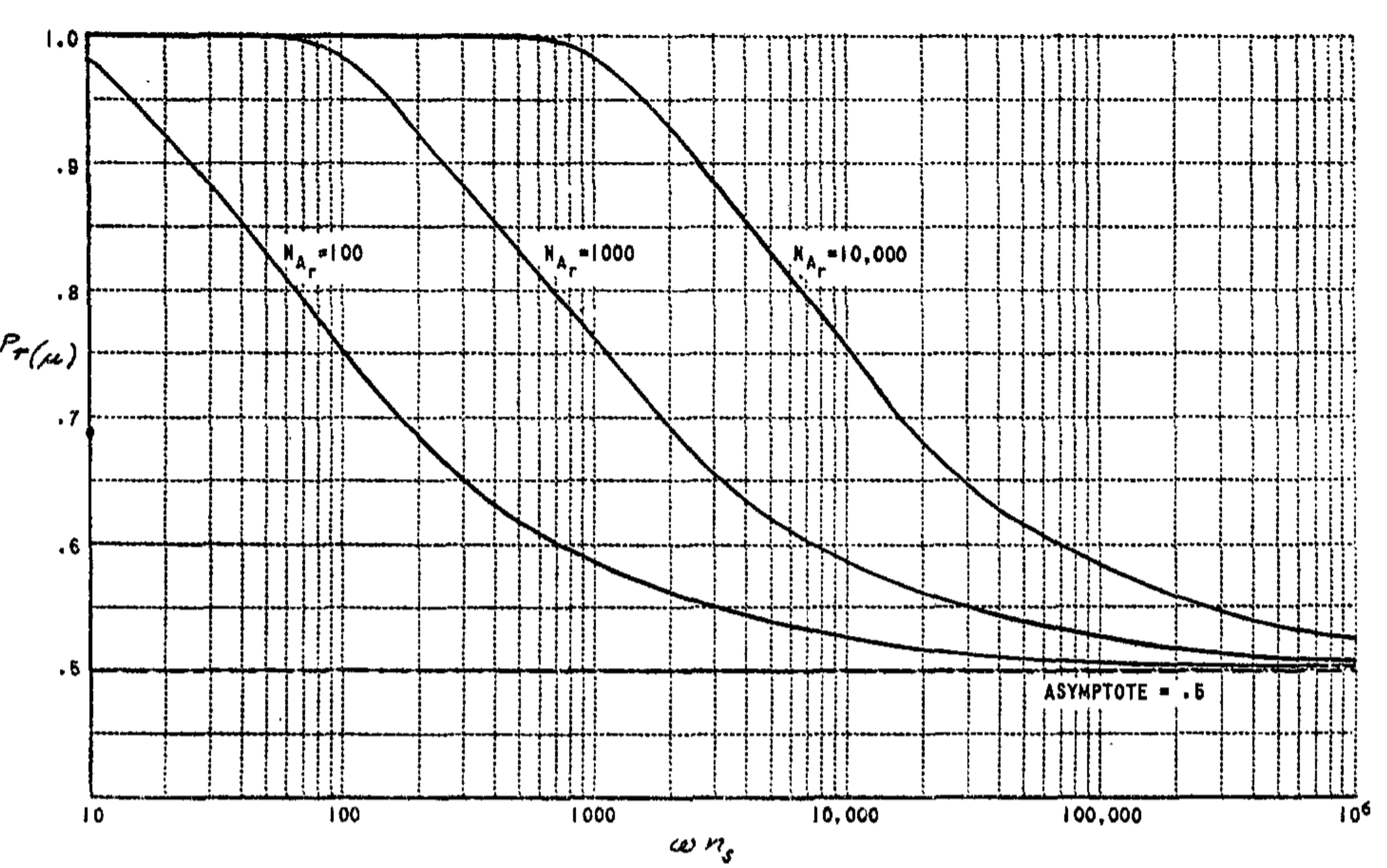
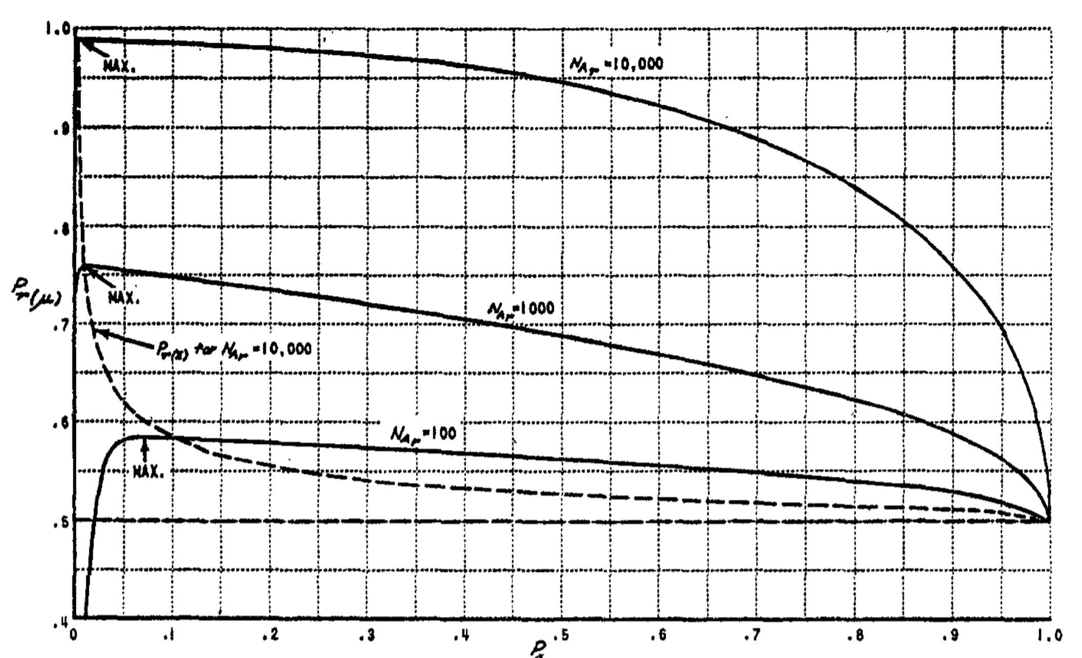
The simplest cases to analyze are those in which the perceptron is shown stimuli drawn from an "ideal environment," consisting of randomly placed points of illumination, where there is no attempt to classify stimuli according to intrinsic similarity. Thus, in a typical learning experiment, we might show the perceptron 1,000 stimuli made up of random collections of illuminated retinal points, and we might arbitrarily reinforce $R_1$ as the "correct" response for the first 500 of these, and $R_2$ for the remaining 500. This environment is "ideal" only in the sense that we speak of an ideal gas in physics; it is a convenient artifact for purposes of analysis, and does not lead to the best performance from the perceptron. In the ideal environment situation, the constant $c_1$ is always equal to zero, so that, in the case of $P_g$ (where $c_2$ is also zero), the value of $Z$ will be zero, and $P_g$ can never be any better than the random expectation of 0.5. The evaluation of $P_r$ for these conditions, however, throws some interesting light on the differences between the alpha, beta, and gamma systems (Table 1).

First consider the alpha system, which has the simplest dynamics of the three. In this system, whenever an A-unit is active for one unit of time, it gains one unit of value. We will assume an experiment, initially, in which $n_{sr}$ (the number of stimuli associated to each response) is constant for all responses. In this case, for the sum system,

$ \left. \begin{aligned} c_1 &= 0 \ c_2 &= (1 - P_a)N_e \ c_3 &= 2P_a \omega \ c_4 &\approx 0 \end{aligned} \right}\tag{5} $

where $\omega = $ the fraction of responses connected to each A-unit. If the source-sets are disjunct, $\omega = 1/N_R$, where $N_R$ is the number of responses in the system. For the $\mu$-system,

$ \left. \begin{aligned} c_1 &= 0 \ c_2 &= (1 - P_a)N_e \ c_3 &= 0 \ c_4 &= 2\omega \end{aligned} \right}\tag{6} $

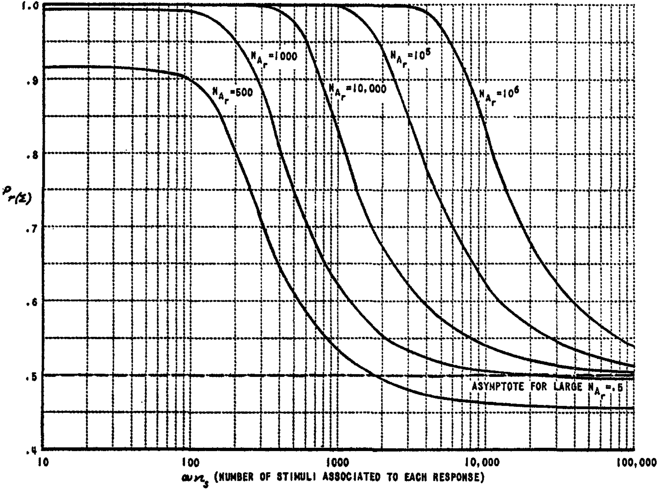
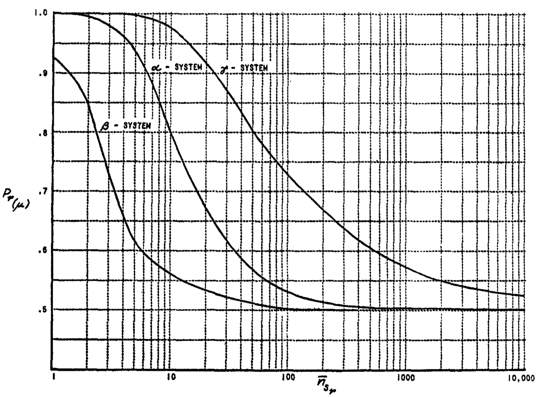
The reduction of $c_3$ to zero gives the $\mu$-system a definite advantage over the $\Sigma$-system. Typical learning curves for these systems are compared in Fig. 7 and 8. Figure 9 shows the effect of variations in $P_a$ upon the performance of the system.

If $n_{sr}$, instead of being fixed, is treated as a random variable, so that the number of stimuli associated to each response is drawn separately from some distribution, then the performance of the $\alpha$-system is considerably poorer than the above equations indicate. Under these conditions, the constants for the $\mu$-system are

$ \left. \begin{aligned} c_1 &= 0 \ c_2 &= 1 - P_a \ c_3 &= 2P_a^2 q^2 \left[ \frac{(\omega N_R - 1)^2}{N_R - 2} + 1 \right] \ c_4 &= \frac{2(1 - P_a)N_R}{(1 - \omega_c)N_A} \end{aligned} \right}\tag{7} $

where $q = $ ratio of $\sigma_{n_{sr}}$ to $\bar{n}_{sr}$ $N_R = $ number of responses in the system $N_A = $ number of A-units in the system $\omega_c = $ proportion of A-units common to $R_1$ and $R_2$.

For this equation (and any others in which $n_{sr}$ is treated as a random variable), it is necessary to define $n_{sr}$ in Equation 4 as the expected value of this variable, over the set of all responses.

For the $\beta$-system, there is an even greater deficit in performance, due to the fact that the net value continues to grow regardless of what happens to the system. The large net values of the subsets activated by a stimulus tend to amplify small statistical differences, causing an unreliable performance. The constants in this case (again for the $\mu$-system) are

$ \left. \begin{aligned} c_1 &= 0 \ c_2 &= (1 - P_a)N_e \ c_3 &= 2(P_a N_e q \omega N_R^2)^2 \ c_4 &= 2(1 - P_a)\omega N_R N_e \end{aligned} \right}\tag{8} $

In both the alpha and beta systems, performance will be poorer for the sum-discriminating model than for the mean-discriminating case. In the gamma-system, however, it can be shown that $P_r(\Sigma) = P_r(\mu)$; i.e., it makes no difference in performance whether the $\Sigma$-system or $\mu$-system is used. Moreover, the constants for the $\gamma$-system, with variable $n_{sr}$, are identical to the constants for the alpha $\mu$-system, with $n_{sr}$ fixed (Equation 6). This demonstrates the advantage of the $\gamma$-system.

Let us now replace the "ideal environment" assumptions with a model for a "differentiated environment," in which several distinguishable classes of stimuli are present (such as squares, circles, and triangles, or the letters of the alphabet). If we then design an experiment in which the stimuli associated to each response are drawn from a different class, then the learning curves of the perceptron are drastically altered. The most important difference is that the constant $c_1$ (the coefficient of $n_{sr}$ in the numerator of $Z$) is no longer equal to zero, so that Equation 4 now has a nonrandom asymptote. Moreover, in the form for $P_g$ (the probability of correct generalization), where $c_2 = 0$, the quantity $Z$ remains greater than zero, and $P_g$ actually approaches the same asymptote as $P_r$. Thus the equation for the perceptron's performance after infinite experience with each class of stimuli is identical for $P_r$ and $P_g$:

$ P_{r_\infty} = P_{g_\infty} = [1 - (1 - P_a)^{N_e}] \times \Phi\left(\frac{c_1}{\sqrt{c_3}}\right)\tag{9} $

This means that in the limit it makes no difference whether the perceptron has seen a particular test stimulus before or not; if the stimuli are drawn from a differentiated environment, the performance will be equally good in either case.

In order to evaluate the performance of the system in a differentiated environment, it is necessary to define the quantity $P_{C_{\alpha\beta}}$. This quantity is interpreted as the expected value of $P_c$ between pairs of stimuli drawn at random from classes $\alpha$ and $\beta$. In particular, $P_{C_{11}}$ is the expected value of $P_c$ between members of the same class, and $P_{C_{12}}$ is the expected value of $P_c$ between an $S_1$ stimulus drawn from Class 1 and an $S_2$ stimulus drawn from Class 2. $P_{C_{1x}}$ is the expected value of $P_c$ between members of Class 1 and stimuli drawn at random from all other classes in the environment.

If $P_{C_{11}} > P_a > P_{C_{12}}$, the limiting performance of the perceptron ($P_{g_\infty}$) will be better than chance, and learning of some response, $R_1$, as the proper "generalization response" for members of Class 1 should eventually occur. If the above inequality is not met, then improvement over chance performance may not occur, and the Class 2 response is likely to occur instead. It can be shown (15) that for most simple geometrical forms, which we ordinarily regard as "similar," the required inequality can be met, if the parameters of the system are properly chosen.

The equation for $P_r$, for the sum-discriminating version of an alpha-perceptron, in a differentiated environment where $n_{sr}$ is fixed for all responses, will have the following expressions for the four coefficients:

$ \left. \begin{aligned} c_1 &= P_A N_e(P_{C_{11}} - P_{C_{12}}) \ c_2 &= P_A N_e(1 - P_{C_{11}}) \ c_3 &= \sum_{r=1,2} P_A \omega \left{ \sum_{i} P_a(1 - P_a) N_e \right. \ &\quad \times [P_{C_{1r}}^2 + \sigma_s^2(P_{C_{1r}}) \ &\quad + \sigma_j^2(P_{C_{1r}}) + (\omega N_R - 1)^2 \ &\quad \times (P_{C_{1z}} + \sigma_s^2(P_{C_{1z}}) \ &\quad + \sigma_j^2(P_{C_{xz}})) + 2(\omega N_R - 1) \ &\quad \cdot (P_{C_{1r}} P_{C_{1x}})] + P_a^2 N_e^2 \ &\quad \times [\sigma_s^2(P_{C_{1r}}) + (\omega N_R - 1)^2 \ &\quad \cdot \sigma_s^2(P_{C_{1x}}) + 2(\omega N_R - 1) \epsilon] } \ c_4 &= \sum_{r=1,2} P_A N_e [P_{C_{1r}} - P_{C_{1r}}^2 \ &\quad - \sigma_s^2(P_{C_{1r}}) - \sigma_j^2(P_{C_{1r}}) \ &\quad + (\omega N_R - 1) (P_{C_{1x}} - P_{C_{1x}}^2 \ &\quad - \sigma_s^2(P_{C_{1x}}) - \sigma_j^2(P_{C_{1x}})) ] \end{aligned} \right}\tag{10} $

where $\sigma_s^2(P_{C_{1r}})$ and $\sigma_s^2(P_{C_{1x}})$ represent the variance of $P_{C_{1r}}$ and $P_{C_{1x}}$ measured over the set of possible test stimuli, $S_t$, and $\sigma_j^2(P_{C_{1r}})$ and $\sigma_j^2(P_{C_{1x}})$ represent the variance of $P_{C_{1r}}$ and $P_{C_{1x}}$ measured over the set of all A-units, $a_j$. $\epsilon = $ covariance of $P_{C_{1r}} P_{C_{1x}}$, which is assumed to be negligible.

The variances which appear in these expressions have not yielded, thus far, to a precise analysis, and can be treated as empirical variables to be determined for the classes of stimuli in question. If the sigma is set equal to half the expected value of the variable, in each case, a conservative estimate can be obtained. When the stimuli of a given class are all of the same shape, and uniformly distributed over the retina, the subscript $s$ variances are equal to zero. $P_g(\Sigma)$ will be represented by the same set of coefficients, except for $c_2$, which is equal to zero, as usual.

For the mean-discriminating system, the coefficients are:

$ \left. \begin{aligned} c_1 &= (P_{C_{11}} - P_{C_{12}}) \ c_2 &= (1 - P_{C_{11}}) \ c_3 &= \sum_{r=1,2} \left[ \frac{1}{P_a(N_e - 1)} - \frac{1}{N_e - 1} \right] \ &\quad \times [\sigma_j^2(P_{C_{1r}}) + (\omega N_R - 1)^2 \ &\quad \times \sigma_j^2(P_{C_{1x}})] + [\sigma_s^2(P_{C_{1r}}) \ &\quad + (\omega N_R - 1)^2 \sigma_s^2(P_{C_{1x}})] \ c_4 &= \sum_{r=1,2} \frac{1}{P_a N_e} [P_{C_{1r}} - P_{C_{1r}}^2 \ &\quad - \sigma_s^2(P_{C_{1r}}) - \sigma_j^2(P_{C_{1r}}) \ &\quad + (\omega N_R - 1)(P_{C_{1x}} - P_{C_{1x}}^2 \ &\quad - \sigma_s^2(P_{C_{1x}}) - \sigma_j^2(P_{C_{1x}}))] \end{aligned} \right}\tag{11} $

Some covariance terms, which are considered negligible, have been omitted here.

A set of typical learning curves for the differentiated environment model is shown in Fig. 11, for the mean-discriminating system. The parameters are based on measurements for a square-circle discrimination problem. Note that the curves for $P_r$ and $P_g$ both approach the same asymptotes, as predicted. The values of these asymptotes can be obtained by substituting the proper coefficients in Equation 9. As the number of association cells in the system increases, the asymptotic learning limit rapidly approaches unity, so that for a system of several thousand cells, the errors in performance should be negligible on a problem as simple as the one illustrated here.

As the number of responses in the system increases, the performance becomes progressively poorer, if every response is made mutually exclusive of all alternatives. One method of avoiding this deterioration (described in detail in Rosenblatt, 15) is through the binary coding of responses. In this case, instead of representing 100 different stimulus patterns by 100 distinct, mutually exclusive responses, a limited number of discriminating features is found, each of which can be independently recognized as being present or absent, and consequently can be represented by a single pair of mutually exclusive responses. Given an ideal set of binary characteristics (such as dark, light; tall, short; straight, curved; etc.), 100 stimulus classes could be distinguished by the proper configuration of only seven response pairs. In a further modification of the system, a single response is capable of denoting by its activity or inactivity the presence or absence of each binary characteristic. The efficiency of such coding depends on the number of independently recognizable "earmarks" that can be found to differentiate stimuli. If the stimulus can be identified only in its entirety and is not amenable to such analysis, then ultimately a separate binary response pair, or bit, is required to denote the presence or absence of each stimulus class (e.g., "dog" or "not dog"), and nothing has been gained over a system where all responses are mutually exclusive.

BIVALENT SYSTEMS

Section Summary: Bivalent systems allow active internal units to either gain or lose value depending on whether reinforcement is positive or negative, unlike earlier models where active units only increased in strength. This setup supports trial-and-error learning through external reward and punishment signals or through internal binary feedback that strengthens correct responses while weakening incorrect ones, which also reduces bias toward frequently occurring stimuli. Simulations and mathematical analysis show these systems reach high accuracy on multi-part responses, though versions relying on excitatory and inhibitory connections prove somewhat less efficient.

In all of the systems analyzed up to this point, the increments of value gained by an active A-unit, as a result of reinforcement or experience, have always been positive, in the sense that an active unit has always gained in its power to activate the responses to which it is connected. In the gamma-system, it is true that some units lose value, but these are always the inactive units, the active ones gaining in proportion to their rate of activity. In a bivalent system, two types of reinforcement are possible (positive and negative), and an active unit may either gain or lose in value, depending on the momentary state of affairs in the system. If the positive and negative reinforcement can be controlled by the application of external stimuli, they become essentially equivalent to "reward" and "punishment," and can be used in this sense by the experimenter. Under these conditions, a perceptron appears to be capable of trial-and-error learning. A bivalent system need not necessarily involve the application of reward and punishment, however. If a binary-coded response system is so organized that there is a single response or response-pair to represent each "bit," or stimulus characteristic that is learned, with positive feedback to its own source-set if the response is "on," and negative feedback (in the sense that active A-units will lose rather than gain in value) if the response is "off," then the system is still bivalent in its characteristics. Such a bivalent system is particularly efficient in reducing some of the bias effects (preference for the wrong response due to greater size or frequency of its associated stimuli) which plague the alternative systems.

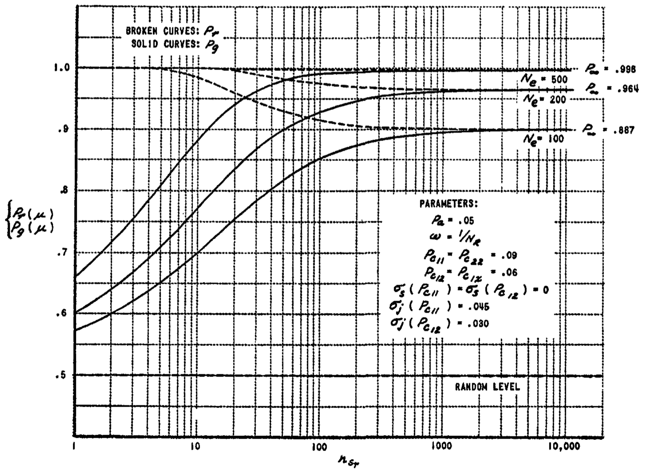
Several forms of bivalent systems have been considered (15, Chap. VII). The most efficient of these has the following logical characteristics. If the system is under a state of positive reinforcement, then a positive $\Delta V$ is added to the values of all active A-units in the source-sets of "on" responses, while a negative $\Delta V$ is added to the active units in the source-sets of "off" responses. If the system is currently under negative reinforcement, then a negative $\Delta V$ is added to all active units in the source-set of an "on" response, and a positive $\Delta V$ is added to active units in an "off" source-set. If the source-sets are disjunct (which is essential for this system to work properly), the equation for a bivalent $\gamma$-system has the same coefficients as the monovalent $\alpha$-system, for the $\mu$-case (Equation 11).

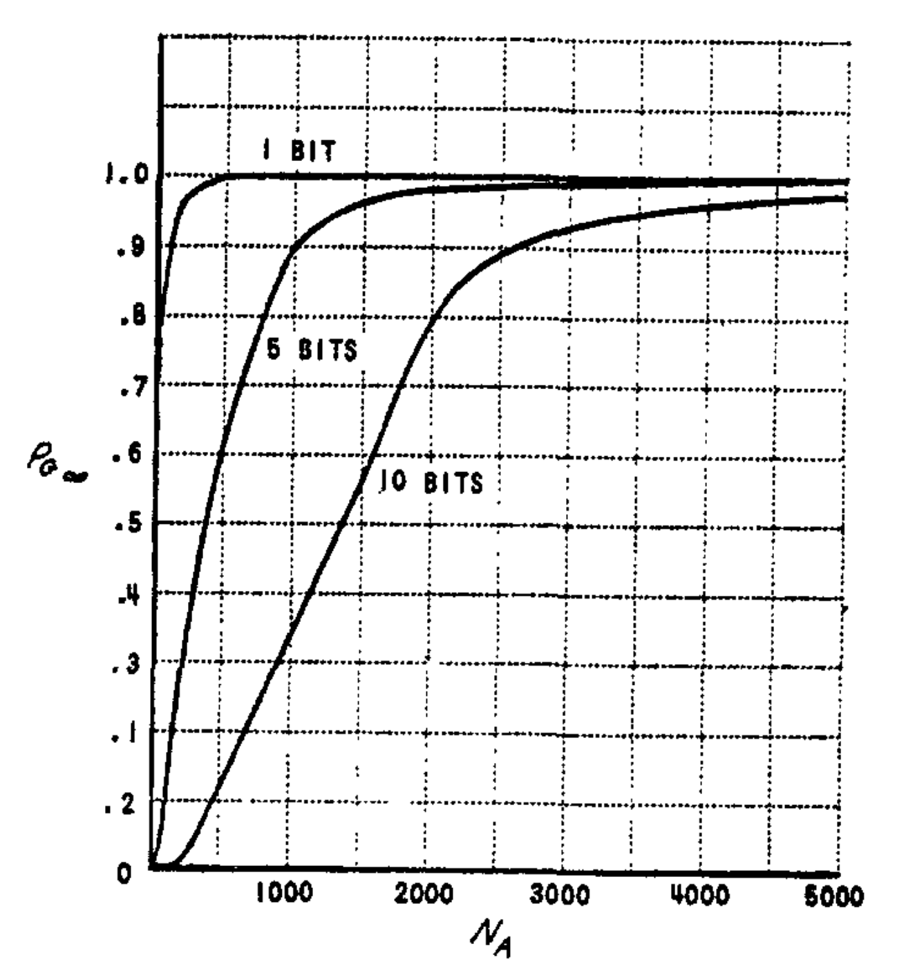
The performance curves for this system are shown in Fig. 12, where the asymptotic generalization probability attainable by the system is plotted for the same stimulus parameters that were used in Fig. 11. This is the probability that all bits in an $n$-bit response pattern will be correct. Clearly, if a majority of correct responses is sufficient to identify a stimulus correctly, the performance will be better than these curves indicate.

In a form of bivalent system which utilizes more plausible biological assumptions, A-units may be either excitatory or inhibitory in their effect on connected responses. A positive $\Delta V$ in this system corresponds to the incrementing of an excitatory unit, while a negative $\Delta V$ corresponds to the incrementing of an inhibitory unit. Such a system performs similarly to the one considered above, but can be shown to be less efficient.

Bivalent systems similar to those illustrated in Fig. 12 have been simulated in detail in a series of experiments with the IBM 704 computer at the Cornell Aeronautical Laboratory. The results have borne out the theory in all of its main predictions, and will be reported separately at a later time.

IMPROVED PERCEPTRONS AND SPONTANEOUS ORGANIZATION

Section Summary: The section explains how perceptrons can be enhanced to handle time-based patterns like motion or sound sequences, provided prior activity leaves a lingering trace in the system, and how spatially organizing input connections improves contour detection. It also describes a decay mechanism in the association units that enables spontaneous concept formation, allowing the device to separate dissimilar stimulus classes through random exposure and unguided reinforcement, as shown in computer simulations. While these features support basic pattern recognition, selective attention, and associative learning across senses, the system still struggles with abstract relationships and relative judgments.

The quantitative analysis of perceptron performance in the preceding sections has omitted any consideration of time as a stimulus dimension. A perceptron which has no capability for temporal pattern recognition is referred to as a "momentary stimulus perceptron." It can be shown (15) that the same principles of statistical separability will permit the perceptron to distinguish velocities, sound sequences, etc., provided the stimuli leave some temporarily persistent trace, such as an altered threshold, which causes the activity in the A-system at time $t$ to depend to some degree on the activity at time $t - 1$.

It has also been assumed that the origin points of A-units are completely random. It can be shown that by a suitable organization of origin points, in which the spatial distribution is constrained (as in the projection area origins shown in Fig. 1), the A-units will become particularly sensitive to the location of contours, and performance will be improved.

In a recent development, which we hope to report in detail in the near future, it has been proven that if the values of the A-units are allowed to decay at a rate proportional to their magnitude, a striking new property emerges: the perceptron becomes capable of "spontaneous" concept formation. That is to say, if the system is exposed to a random series of stimuli from two "dissimilar" classes, and all of its responses are automatically reinforced without any regard to whether they are "right" or "wrong," the system will tend towards a stable terminal condition in which (for each binary response) the response will be "1" for members of one stimulus class, and "0" for members of the other class; i.e., the perceptron will spontaneously recognize the difference between the two classes. This phenomenon has been successfully demonstrated in simulation experiments, with the 704 computer.

A perceptron, even with a single logical level of A-units and response units, can be shown to have a number of interesting properties in the field of selective recall and selective attention. These properties generally depend on the intersection of the source sets for different responses, and are elsewhere discussed in detail (15). By combining audio and photo inputs, it is possible to associate sounds, or auditory "names" to visual objects, and to get the perceptron to perform such selective responses as are designated by the command "Name the object on the left," or "Name the color of this stimulus."

The question may well be raised at this point of where the perceptron's capabilities actually stop. We have seen that the system described is sufficient for pattern recognition, associative learning, and such cognitive sets as are necessary for selective attention and selective recall. The system appears to be potentially capable of temporal pattern recognition, as well as spatial recognition, involving any sensory modality or combination of modalities. It can be shown that with proper reinforcement it will be capable of trial-and-error learning, and can learn to emit ordered sequences of responses, provided its own responses are fed back through sensory channels.

Does this mean that the perceptron is capable, without further modification in principle, of such higher order functions as are involved in human speech, communication, and thinking? Actually, the limit of the perceptron's capabilities seems to lie in the area of relative judgment, and the abstraction of relationships. In its "symbolic behavior," the perceptron shows some striking similarities to Goldstein's brain-damaged patients (5). Responses to definite, concrete stimuli can be learned, even when the proper response calls for the recognition of a number of simultaneous qualifying conditions (such as naming the color if the stimulus is on the left, the shape if it is on the right). As soon as the response calls for the recognition of a relationship between stimuli (such as "Name the object left of the square." or "Indicate the pattern that appeared before the circle."), however, the problem generally becomes excessively difficult for the perceptron. Statistical separability alone does not provide a sufficient basis for higher order abstraction. Some system, more advanced in principle than the perceptron, seems to be required at this point.

CONCLUSIONS AND EVALUATION

Section Summary: The theoretical analysis concludes that a randomly connected perceptron system can learn stimulus-response associations and generalize to new inputs in environments where stimuli fall into correlated classes, with accuracy improving as the number of association units grows and memory distributed across the network rather than localized. These abilities, along with features such as contour sensitivity and binary outputs, emerge directly from a handful of measurable physical parameters like connection counts, thresholds, and unit quantities. Compared with prior learning theories based mainly on fitting behavioral data, the model gains parsimony and verifiability by needing only one hypothetical construct whose physical basis can be tested independently.

The main conclusions of the theoretical study of the perceptron can be summarized as follows:

1. In an environment of random stimuli, a system consisting of randomly connected units, subject to the parametric constraints discussed above, can learn to associate specific responses to specific stimuli. Even if many stimuli are associated to each response, they can still be recognized with a better-than-chance probability, although they may resemble one another closely and may activate many of the same sensory inputs to the system.
2. In such an "ideal environment," the probability of a correct response diminishes towards its original random level as the number of stimuli learned increases.
3. In such an environment, no basis for generalization exists.
4. In a "differentiated environment," where each response is associated to a distinct class of mutually correlated, or "similar" stimuli, the probability that a learned association of some specific stimulus will be correctly retained typically approaches a better-than-chance asymptote as the number of stimuli learned by the system increases. This asymptote can be made arbitrarily close to unity by increasing the number of association cells in the system.
5. In the differentiated environment, the probability that a stimulus which has not been seen before will be correctly recognized and associated to its appropriate class (the probability of correct generalization) approaches the same asymptote as the probability of a correct response to a previously reinforced stimulus. This asymptote will be better than chance if the inequality $P_{C_{12}} < P_a < P_{C_{11}}$ is met, for the stimulus classes in question.
6. The performance of the system can be improved by the use of a contour-sensitive projection area, and by the use of a binary response system, in which each response, or "bit," corresponds to some independent feature or attribute of the stimulus.
7. Trial-and-error learning is possible in bivalent reinforcement systems.
8. Temporal organizations of both stimulus patterns and responses can be learned by a system which uses only an extension of the original principles of statistical separability, without introducing any major complications in the organization of the system.
9. The memory of the perceptron is distributed, in the sense that any association may make use of a large proportion of the cells in the system, and the removal of a portion of the association system would not have an appreciable effect on the performance of any one discrimination or association, but would begin to show up as a general deficit in all learned associations.
10. Simple cognitive sets, selective recall, and spontaneous recognition of the classes present in a given environment are possible. The recognition of relationships in space and time, however, seems to represent a limit to the perceptron's ability to form cognitive abstractions.

Psychologists, and learning theorists in particular, may now ask: "What has the present theory accomplished, beyond what has already been done in the quantitative theories of Hull, Bush and Mosteller, etc., or physiological theories such as Hebb's?" The present theory is still too primitive, of course, to be considered as a full-fledged rival of existing theories of human learning. Nonetheless, as a first approximation, its chief accomplishment might be stated as follows: For a given mode of organization ($\alpha, \beta$, or $\gamma; \Sigma$ or $\mu$; monovalent or bivalent) the fundamental phenomena of learning, perceptual discrimination, and generalization can be predicted entirely from six basic physical parameters, namely:

$x$: the number of excitatory connections per A-unit, $y$: the number of inhibitory connections per A-unit, $\theta$: the expected threshold of an A-unit, $\omega$: the proportion of R-units to which an A-unit is connected, $N_A$: the number of A-units in the system, and $N_R$: the number of R-units in the system.

$N_s$ (the number of sensory units) becomes important if it is very small. It is assumed that the system begins with all units in a uniform state of value; otherwise the initial value distribution would also be required. Each of the above parameters is a clearly defined physical variable, which is measurable in its own right, independently of the behavioral and perceptual phenomena which we are trying to predict.

As a direct consequence of its foundation on physical variables, the present system goes far beyond existing learning and behavior theories in three main points: parsimony, verifiability, and explanatory power and generality. Let us consider each of these points in turn.

1. Parsimony. Essentially all of the basic variables and laws used in this system are already present in the structure of physical and biological science, so that we have found it necessary to postulate only one hypothetical variable (or construct) which we have called V, the "value" of an association cell; this is a variable which must conform to certain functional characteristics which can clearly be stated, and which is assumed to have a potentially measurable physical correlate.
2. Verifiability. Previous quantitative learning theories, apparently without exception, have had one important characteristic in common: they have all been based on measurements of behavior, in specified situations, using these measurements (after theoretical manipulation) to predict behavior in other situations. Such a procedure, in the last analysis, amounts to a process of curve fitting and extrapolation, in the hope that the constants which describe one set of curves will hold good for other curves in other situations. While such extrapolation is not necessarily circular, in the strict sense, it shares many of the logical difficulties of circularity, particularly when used as an "explanation" of behavior. Such extrapolation is difficult to justify in a new situation, and it has been shown that if the basic constants and parameters are to be derived anew for any situation in which they break down empirically (such as change from white rats to humans), then the basic "theory" is essentially irrefutable, just as any successful curve-fitting equation is irrefutable. It has, in fact, been widely conceded by psychologists that there is little point in trying to "disprove" any of the major learning theories in use today, since by extension, or a change in parameters, they have all proved capable of adapting to any specific empirical data. This is epitomized in the increasingly common attitude that a choice of theoretical model is mostly a matter of personal aesthetic preference or prejudice, each scientist being entitled to a favorite model of his own. In considering this approach, one is reminded of a remark attributed to Kistiakowsky, that "given seven parameters, I could fit an elephant." This is clearly not the case with a system in which the independent variables, or parameters, can be measured independently of the predicted behavior. In such a system, it is not possible to "force" a fit to empirical data, if the parameters in current use should lead to improper results. In the current theory, a failure to fit a curve in a new situation would be a clear indication that either the theory or the empirical measurements are wrong. Consequently, if such a theory does hold up for repeated tests, we can be considerably more confident of its validity and of its generality than in the case of a theory which must be hand-tailored to meet each situation.
3. Explanatory power and generality. The present theory, being derived from basic physical variables, is not specific to any one organism or learning situation. It can be generalized in principle to cover any form of behavior in any system for which the physical parameters are known. A theory of learning, constructed on these foundations, should be considerably more powerful than any which has previously been proposed. It would not only tell us what behavior might occur in any known organism, but would permit the synthesis of behaving systems, to meet special requirements. Other learning theories tend to become increasingly qualitative as they are generalized. Thus a set of equations describing the effects of reward on T-maze learning in a white rat reduces simply to a statement that rewarded behavior tends to occur with increasing probability, when we attempt to generalize it from any species and any situation. The theory which has been presented here loses none of its precision through generality.

The theory proposed by Donald Hebb (7) attempts to avoid these difficulties of behavior-based models by showing how psychological functioning might be derived from neuro-physiological theory. In his attempt to achieve this, Hebb's philosophy of approach seems close to our own, and his work has been a source of inspiration for much of what has been proposed here. Hebb, however, has never actually achieved a model by which behavior (or any psychological data) can be predicted from the physiological system. His physiology is more a suggestion as to the sort of organic substrate which might underlie behavior, and an attempt to show the plausibility of a bridge between biophysics and psychology.

The present theory represents the first actual completion of such a bridge. Through the use of the equations in the preceding sections, it is possible to predict learning curves from neurological variables, and likewise, to predict neurological variables from learning curves. How well this bridge stands up to repeated crossings remains to be seen. In the meantime, the theory reported here clearly demonstrates the feasibility and fruitfulness of a quantitative statistical approach to the organization of cognitive systems. By the study of systems such as the perceptron, it is hoped that those fundamental laws of organization which are common to all information handling systems, machines and men included, may eventually be understood.

REFERENCES

Section Summary: This reference list compiles 18 books and journal articles, mostly published between 1938 and 1958, that address brain function, behavior, perception, and early ideas about machines modeling mental processes. The works come from fields such as neurophysiology, psychology, and mathematical biology, with several contributions appearing in edited volumes on automata and cerebral mechanisms. The section closes with the date the source paper was received.

1. ASHBY, W. R. Design for a brain. New York: Wiley, 1952.

2. CULBERTSON, J. T. Consciousness and behavior. Dubuque, Iowa: Wm. C. Brown, 1950.

3. CULBERTSON, J. T. Some uneconomical robots. In C. E. Shannon & J. McCarthy (Eds.), Automata studies. Princeton: Princeton Univer. Press, 1956. Pp. 99-116.

4. ECCLES, J. C. The neurophysiological basis of mind. Oxford: Clarendon, 1953.

5. GOLDSTEIN, K. Human nature in the light of psychopathology. Cambridge: Harvard Univer. Press, 1940.

6. HAYEK, F. A. The sensory order. Chicago: Univer. Chicago Press, 1952.

7. HEBB, D. O. The organization of behavior. New York: Wiley, 1949.

8. KLEENE, S. C. Representation of events in nerve nets and finite automata. In C. E. Shannon & J. McCarthy (Eds.), Automata studies. Princeton: Princeton Univer. Press, 1956. Pp. 3-41.

9. KÖHLER, W. Relational determination in perception. In L. A. Jeffress (Ed.), Cerebral mechanisms in behavior. New York: Wiley, 1951. Pp. 200-243.

10. MCCULLOCH, W. S. Why the mind is in the head. In L. A. Jeffress (Ed.), Cerebral mechanisms in behavior. New York: Wiley, 1951. Pp. 42-111.

11. MCCULLOCH, W. S., & PITTS, W. A logical calculus of the ideas immanent in nervous activity. Bull. math. Biophysics, 1943, 5, 115-133.

12. MILNER, P. M. The cell assembly: Mark II. Psychol. Rev., 1957, 64, 242-252.

13. MINSKY, M. L. Some universal elements for finite automata. In C. E. Shannon & J. McCarthy (Eds.), Automata studies. Princeton: Princeton Univer. Press, 1956. Pp. 117-128.

14. RASHEVSKY, N. Mathematical biophysics. Chicago: Univer. Chicago Press, 1938.

15. ROSENBLATT, F. The perceptron: A theory of statistical separability in cognitive systems. Buffalo: Cornell Aeronautical Laboratory, Inc. Rep. No. VG-1196-G-1, 1958.

16. UTTLEY, A. M. Conditional probability machines and conditioned reflexes. In C. E. Shannon & J. McCarthy (Eds.), Automata studies. Princeton: Princeton Univer. Press, 1956. Pp. 253-275.

17. VON NEUMANN, J. The general and logical theory of automata. In L. A. Jeffress (Ed.), Cerebral mechanisms in behavior. New York: Wiley, 1951. Pp. 1-41.

18. VON NEUMANN, J. Probabilistic logics and the synthesis of reliable organisms from unreliable components. In C. E. Shannon & J. McCarthy (Eds.), Automata studies. Princeton: Princeton Univer. Press, 1956. Pp. 43-98.

(Received April 23, 1958)