Algorithms for Hyper-Parameter Optimization

James Bergstra
The Rowland Institute
Harvard University
[email protected]

Rémi Bardenet
Laboratoire de Recherche en Informatique
Université Paris-Sud
[email protected]

Yoshua Bengio
Dépt. d’Informatique et Recherche Opérationelle
Université de Montréal
[email protected]

Balázs Kégl
Linear Accelerator Laboratory
Université Paris-Sud, CNRS
[email protected]

Abstract

Several recent advances to the state of the art in image classification benchmarks have come from better configurations of existing techniques rather than novel approaches to feature learning. Traditionally, hyper-parameter optimization has been the job of humans because they can be very efficient in regimes where only a few trials are possible. Presently, computer clusters and GPU processors make it possible to run more trials and we show that algorithmic approaches can find better results. We present hyper-parameter optimization results on tasks of training neural networks and deep belief networks (DBNs). We optimize hyper-parameters using random search and two new greedy sequential methods based on the expected improvement criterion. Random search has been shown to be sufficiently efficient for learning neural networks for several datasets, but we show it is unreliable for training DBNs. The sequential algorithms are applied to the most difficult DBN learning problems from [1] and find significantly better results than the best previously reported. This work contributes novel techniques for making response surface models $P(y|x)$ in which many elements of hyper-parameter assignment ($x$) are known to be irrelevant given particular values of other elements.

Executive Summary: The paper addresses the challenge of tuning hyper-parameter configurations for complex machine learning models such as deep belief networks, which can involve up to 32 variables including discrete, continuous, and conditional choices. Manual tuning by experts has long been the standard approach, yet it is slow, difficult to reproduce, and increasingly mismatched to modern hardware that supports many more trials. The work evaluates whether algorithmic methods can locate better configurations than either manual search or simple random sampling on established image-classification benchmarks.

The authors set out to compare random search against two new sequential model-based optimization procedures that use an expected-improvement criterion to propose successive trials. One procedure builds a hierarchical Gaussian-process surrogate; the other uses a tree-structured Parzen estimator that models the conditional density of promising configurations. Both methods were run on the two hardest datasets from an earlier manual study, with a budget of 200 trials each, and the resulting models were evaluated on held-out test data.

Random search matched or slightly exceeded the performance of the original manual search on several datasets when allowed a comparable number of trials. On the two most difficult tasks, however, the sequential algorithms produced clear gains. The Parzen-estimator method reached 14.1 % test error on the convex dataset (versus 18.6 % for manual search and 19.0 % for random search) and 44.6 % on the rotated-background-images task (versus 47.4 % and 50.5 %, respectively). The Gaussian-process method performed between the manual baseline and the Parzen estimator. Both sequential procedures completed their 200-trial searches in roughly 24 hours of wall-clock time on five GPUs.

These results indicate that automated hyper-parameter search can reliably surpass expert manual tuning on realistic, high-dimensional problems and that the gains are large enough to matter for benchmark performance. The availability of an open-source implementation of the stronger of the two methods removes a practical barrier to wider adoption.

The main limitations are that the experiments focus on deep belief networks and that the sequential procedures can be misled by an inaccurate surrogate model, although no such failure occurred in the reported runs. Overall, the evidence supports replacing or augmenting manual tuning with these algorithmic approaches whenever sufficient compute is available.

1 Introduction

Section Summary: Complex machine learning models like deep belief networks often involve dozens of hyperparameters whose tuning is difficult and somewhat arbitrary, making results hard to reproduce and progress more of an art than a science. The paper shows that systematic hyperparameter search, rather than new modeling ideas alone, can drive major gains in performance, and that the search space itself can be described as a generative process over tree-structured choices mixing discrete, ordinal, and continuous variables. It reports that simply drawing random configurations from this process already rivals careful manual tuning, while sequential automatic methods outperform both.

Models such as Deep Belief Networks (DBNs) [2], stacked denoising autoencoders [3], convolutional networks [4], as well as classifiers based on sophisticated feature extraction techniques have from ten to perhaps fifty hyper-parameters, depending on how the experimenter chooses to parametrize the model, and how many hyper-parameters the experimenter chooses to fix at a reasonable default. The difficulty of tuning these models makes published results difficult to reproduce and extend, and makes even the original investigation of such methods more of an art than a science.

Recent results such as [5], [6], and [7] demonstrate that the challenge of hyper-parameter optimization in large and multilayer models is a direct impediment to scientific progress. These works have advanced state of the art performance on image classification problems by more concerted hyper-parameter optimization in simple algorithms, rather than by innovative modeling or machine learning strategies. It would be wrong to conclude from a result such as [5] that feature learning is useless. Instead, hyper-parameter optimization should be regarded as a formal outer loop in the learning process. A learning algorithm, as a functional from data to classifier (taking classification problems as an example), includes a budgeting choice of how many CPU cycles are to be spent on hyper-parameter exploration, and how many CPU cycles are to be spent evaluating each hyper-parameter choice (i.e. by tuning the regular parameters). The results of [5] and [7] suggest that with current generation hardware such as large computer clusters and GPUs, the optimal allocation of CPU cycles includes more hyper-parameter exploration than has been typical in the machine learning literature.

Hyper-parameter optimization is the problem of optimizing a loss function over a graph-structured configuration space. In this work we restrict ourselves to tree-structured configuration spaces. Configuration spaces are tree-structured in the sense that some leaf variables (e.g. the number of hidden units in the 2nd layer of a DBN) are only well-defined when node variables (e.g. a discrete choice of how many layers to use) take particular values. Not only must a hyper-parameter optimization algorithm optimize over variables which are discrete, ordinal, and continuous, but it must simultaneously choose which variables to optimize.

In this work we define a configuration space by a generative process for drawing valid samples. Random search is the algorithm of drawing hyper-parameter assignments from that process and evaluating them. Optimization algorithms work by identifying hyper-parameter assignments that could have been drawn, and that appear promising on the basis of the loss function's value at other points. This paper makes two contributions: 1) Random search is competitive with the manual optimization of DBNs in [1], and 2) Automatic sequential optimization outperforms both manual and random search.

Section 2 covers sequential model-based optimization, and the expected improvement criterion. Section 3 introduces a Gaussian Process based hyper-parameter optimization algorithm. Section 4 introduces a second approach based on adaptive Parzen windows. Section 5 describes the problem of DBN hyper-parameter optimization, and shows the efficiency of random search. Section 6 shows the efficiency of sequential optimization on the two hardest datasets according to random search. The paper concludes with discussion of results and concluding remarks in Section 7 and Section 8.

2 Sequential Model-based Global Optimization

Section Summary: Sequential Model-Based Global Optimization (SMBO) methods address problems where directly evaluating an objective or fitness function is too slow or costly by instead building a cheaper surrogate model of that function from past observations. In each step the algorithm optimizes a chosen criterion on the surrogate, such as expected improvement over the best value seen so far, to decide where to evaluate the true function next, then updates the model with the new result. The paper focuses on two new ways to construct the surrogate from data—a hierarchical Gaussian process and a tree-structured Parzen estimator—while using expected improvement as the selection criterion.

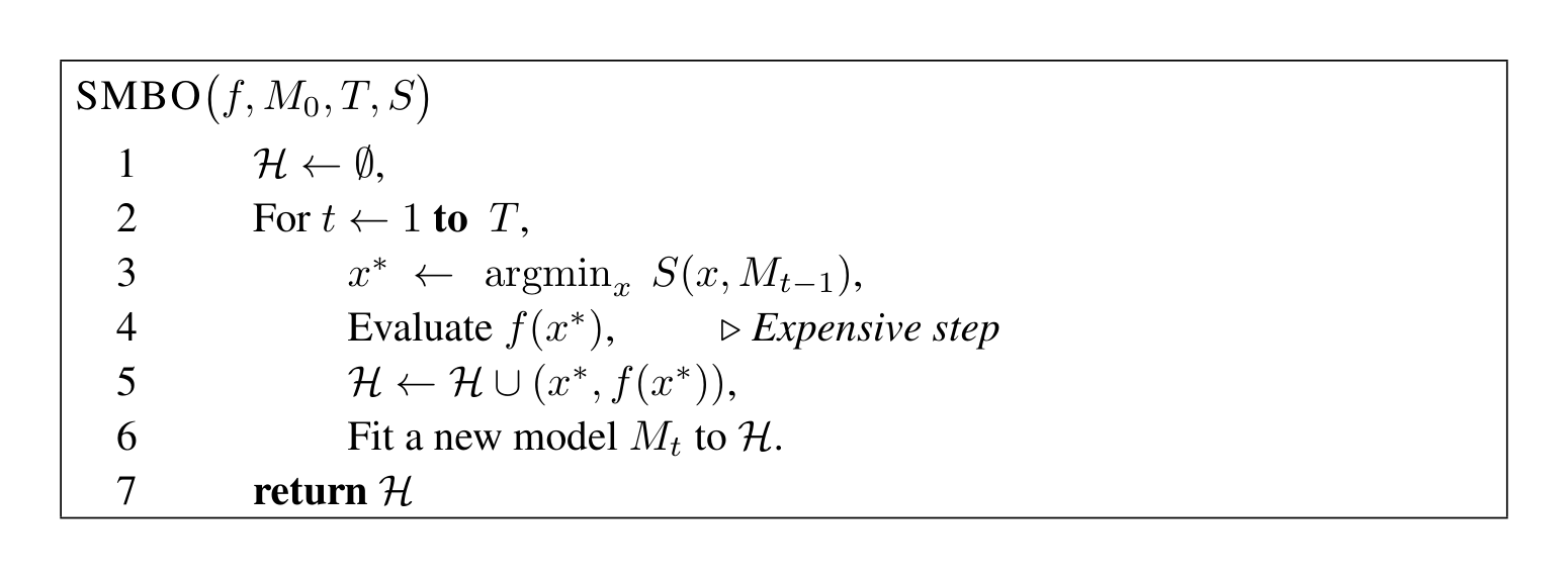
Sequential Model-Based Global Optimization (SMBO) algorithms have been used in many applications where evaluation of the fitness function is expensive [8, 9]. In an application where the true fitness function $f : \mathcal{X} \rightarrow \mathbb{R}$ is costly to evaluate, model-based algorithms approximate $f$ with a surrogate that is cheaper to evaluate. Typically the inner loop in an SMBO algorithm is the numerical optimization of this surrogate, or some transformation of the surrogate. The point $x^*$ that maximizes the surrogate (or its transformation) becomes the proposal for where the true function $f$ should be evaluated. This active-learning-like algorithm template is summarized in Figure 1. SMBO algorithms differ in what criterion they optimize to obtain $x^*$ given a model (or surrogate) of $f$, and in they model $f$ via observation history $\mathcal{H}$.

The algorithms in this work optimize the criterion of Expected Improvement (EI) [10]. Other criteria have been suggested, such as Probability of Improvement and Expected Improvement [10], minimizing the Conditional Entropy of the Minimizer [11], and the bandit-based criterion described in [12]. We chose to use the EI criterion in our work because it is intuitive, and has been shown to work well in a variety of settings. We leave the systematic exploration of improvement criteria for future work. Expected improvement is the expectation under some model $M$ of $f : \mathcal{X} \rightarrow \mathbb{R}^N$ that $f(x)$ will exceed (negatively) some threshold $y^*$:

$ \text{EI}{y^*}(x) := \int{-\infty}^{\infty} \max(y^* - y, 0) p_M(y|x) dy.\tag{1} $

The contribution of this work is two novel strategies for approximating $f$ by modeling $\mathcal{H}$: a hierarchical Gaussian Process and a tree-structured Parzen estimator. These are described in Section 3 and Section 4 respectively.

3 The Gaussian Process Approach (GP)

Section Summary: Gaussian Processes serve as a flexible statistical model for approximating an unknown loss function during hyperparameter tuning, since they update their predictions and uncertainty estimates analytically after each new observation and naturally balance promising regions against unexplored ones through the expected-improvement criterion. To locate the next point to evaluate, the method optimizes this criterion with a hybrid evolutionary search that applies CMA-ES to continuous parameters and binomial sampling to discrete ones, restarting the search multiple times from promising locations. Because many hyperparameters are only meaningful for certain model architectures, separate independent GPs are placed over logically grouped subsets of parameters arranged in a tree structure.

Gaussian Processes have long been recognized as a good method for modeling loss functions in model-based optimization literature [13]. Gaussian Processes (GPs, [14]) are priors over functions that are closed under sampling, which means that if the prior distribution of $f$ is believed to be a GP with mean 0 and kernel $k$, the conditional distribution of $f$ knowing a sample $\mathcal{H} = (x_i, f(x_i))_{i=1}^n$ of its values is also a GP, whose mean and covariance function are analytically derivable. GPs with generic mean functions can in principle be used, but it is simpler and sufficient for our purposes to only consider zero mean processes. We do this by centering the function values in the considered data sets. Modelling e.g. linear trends in the GP mean leads to undesirable extrapolation in unexplored regions during SMBO [15].

The above mentioned closedness property, along with the fact that GPs provide an assessment of prediction uncertainty incorporating the effect of data scarcity, make the GP an elegant candidate for both finding candidate $x^*$ (Figure 1, step 3) and fitting a model $M_t$ (Figure 1, step 6). The runtime of each iteration of the GP approach scales cubically in $|\mathcal{H}|$ and linearly in the number of variables being optimized, however the expense of the function evaluations $f(x^*)$ typically dominate even this cubic cost.

3.1 Optimizing EI in the GP

We model $f$ with a GP and set $y^*$ to the best value found after observing $\mathcal{H}$: $y^* = \min{f(x_i), 1 \leq i \leq n}$. The model $p_M$ in (1) is then the posterior GP knowing $\mathcal{H}$. The EI function in (1) encapsulates a compromise between regions where the mean function is close to or better than $y^*$ and under-explored regions where the uncertainty is high.

EI functions are usually optimized with an exhaustive grid search over the input space, or a Latin Hypercube search in higher dimensions. However, some information on the landscape of the EI criterion can be derived from simple computations [16]: 1) it is always non-negative and zero at training points from $\mathcal{D}$, 2) it inherits the smoothness of the kernel $k$, which is in practice often at least once differentiable, and noticeably, 3) the EI criterion is likely to be highly multi-modal, especially as the number of training points increases. The authors of [16] used the preceding remarks on the landscape of EI to design an evolutionary algorithm with mixture search, specifically aimed at optimizing EI, that is shown to outperform exhaustive search for a given budget in EI evaluations. We borrow here their approach and go one step further. We keep the Estimation of Distribution (EDA, [17]) approach on the discrete part of our input space (categorical and discrete hyper-parameters), where we sample candidate points according to binomial distributions, while we use the Covariance Matrix Adaptation - Evolution Strategy (CMA-ES, [18]) for the remaining part of our input space (continuous hyper-parameters). CMA-ES is a state-of-the-art gradient-free evolutionary algorithm for optimization on continuous domains, which has been shown to outperform the Gaussian search EDA. Notice that such a gradient-free approach allows non-differentiable kernels for the GP regression. We do not take on the use of mixtures in [16], but rather restart the local searches several times, starting from promising places. The use of tesselations suggested by [16] is prohibitive here, as our task often means working in more than 10 dimensions, thus we start each local search at the center of mass of a simplex with vertices randomly picked among the training points.

Finally, we remark that all hyper-parameters are not relevant for each point. For example, a DBN with only one hidden layer does not have parameters associated to a second or third layer. Thus it is not enough to place one GP over the entire space of hyper-parameters. We chose to group the hyper-parameters by common use in a tree-like fashion and place different independent GPs over each group. As an example, for DBNs, this means placing one GP over common hyper-parameters, including categorical parameters that indicate what are the conditional groups to consider, three GPs on the parameters corresponding to each of the three layers, and a few 1-dimensional GPs over individual conditional hyper-parameters, like ZCA energy (see Table 1 for DBN parameters).

4 Tree-structured Parzen Estimator Approach (TPE)

Section Summary: The Tree-structured Parzen Estimator (TPE) is an alternative strategy for hyper-parameter search that models the probability of different configurations given their observed performance, rather than modeling performance given a configuration. It represents the space of possible settings through a hierarchical generative process and replaces the original priors with simple non-parametric densities, such as mixtures of truncated Gaussians or re-weighted categorical distributions, built separately from the better and worse observed results. By choosing a performance threshold that splits these two groups, the method directly maximizes expected improvement by favoring new points that are more probable under the density of good results, while scaling linearly with the number of observations and dimensions.

Anticipating that our hyper-parameter optimization tasks will mean high dimensions and small fitness evaluation budgets, we now turn to another modeling strategy and EI optimization scheme for the SMBO algorithm. Whereas the Gaussian-process based approach modeled $p(y|x)$ directly, this strategy models $p(x|y)$ and $p(y)$.

Recall from the introduction that the configuration space $\mathcal{X}$ is described by a graph-structured generative process (e.g. first choose a number of DBN layers, then choose the parameters for each). The tree-structured Parzen estimator (TPE) models $p(x|y)$ by transforming that generative process, replacing the distributions of the configuration prior with non-parametric densities. In the experimental section, we will see that the configuration space is described using uniform, log-uniform, quantized log-uniform, and categorical variables. In these cases, the TPE algorithm makes the following replacements: uniform $\rightarrow$ truncated Gaussian mixture, log-uniform $\rightarrow$ exponentiated truncated Gaussian mixture, categorical $\rightarrow$ re-weighted categorical. Using different observations ${x^{(1)}, \dots, x^{(k)}}$ in the non-parametric densities, these substitutions represent a learning algorithm that can produce a variety of densities over the configuration space $\mathcal{X}$. The TPE defines $p(x|y)$ using two such densities:

$ p(x|y) = \begin{cases} \ell(x) & \text{if } y < y^* \ g(x) & \text{if } y \ge y^*, \end{cases}\tag{2} $

where $\ell(x)$ is the density formed by using the observations ${x^{(i)}}$ such that corresponding loss $f(x^{(i)})$ was less than $y^*$ and $g(x)$ is the density formed by using the remaining observations. Whereas the GP-based approach favoured quite an aggressive $y^*$ (typically less than the best observed loss), the TPE algorithm depends on a $y^*$ that is larger than the best observed $f(x)$ so that some points can be used to form $\ell(x)$. The TPE algorithm chooses $y^*$ to be some quantile $\gamma$ of the observed $y$ values, so that $p(y < y^*) = \gamma$, but no specific model for $p(y)$ is necessary. By maintaining sorted lists of observed variables in $\mathcal{H}$, the runtime of each iteration of the TPE algorithm can scale linearly in $|\mathcal{H}|$ and linearly in the number of variables (dimensions) being optimized.

4.1 Optimizing EI in the TPE algorithm

The parametrization of $p(x, y)$ as $p(y)p(x|y)$ in the TPE algorithm was chosen to facilitate the optimization of EI.

$ \text{EI}{y^*}(x) = \int{-\infty}^{y^*} (y^* - y) p(y|x) dy = \int_{-\infty}^{y^*} (y^* - y) \frac{p(x|y)p(y)}{p(x)} dy\tag{3} $

By construction, $\gamma = p(y < y^*)$ and $p(x) = \int_{\mathbb{R}} p(x|y)p(y)dy = \gamma \ell(x) + (1 - \gamma)g(x)$. Therefore

$ \int_{-\infty}^{y^*} (y^* - y)p(x|y)p(y)dy = \ell(x) \int_{-\infty}^{y^*} (y^* - y)p(y)dy = \gamma y^* \ell(x) - \ell(x) \int_{-\infty}^{y^*} p(y)dy, $

so that finally $\text{EI}{y^*}(x) = \frac{\gamma y^* \ell(x) - \ell(x) \int{-\infty}^{y^*} p(y)dy}{\gamma \ell(x) + (1 - \gamma)g(x)} \propto \left( \gamma + \frac{g(x)}{\ell(x)}(1 - \gamma) \right)^{-1}$. This last expression shows that to maximize improvement we would like points $x$ with high probability under $\ell(x)$ and low probability under $g(x)$. The tree-structured form of $\ell$ and $g$ makes it easy to draw many candidates according to $\ell$ and evaluate them according to $g(x)/\ell(x)$. On each iteration, the algorithm returns the candidate $x^*$ with the greatest EI.

4.2 Details of the Parzen Estimator

The models $\ell(x)$ and $g(x)$ are hierarchical processes involving discrete-valued and continuous-valued variables. The Adaptive Parzen Estimator yields a model over $\mathcal{X}$ by placing density in the vicinity of $K$ observations $\mathcal{B} = {x^{(1)}, \dots, x^{(K)}} \subset \mathcal{H}$. Each continuous hyper-parameter was specified by a uniform prior over some interval $(a, b)$, or a Gaussian, or a log-uniform distribution. The TPE substitutes an equally-weighted mixture of that prior with Gaussians centered at each of the $x^{(i)} \in \mathcal{B}$. The standard deviation of each Gaussian was set to the greater of the distances to the left and right neighbor, but clipped to remain in a reasonable range. In the case of the uniform, the points $a$ and $b$ were considered to be potential neighbors. For discrete variables, supposing the prior was a vector of $N$ probabilities $p_i$, the posterior vector elements were proportional to $N p_i + C_i$ where $C_i$ counts the occurrences of choice $i$ in $\mathcal{B}$. The log-uniform hyper-parameters were treated as uniforms in the log domain.

: Table 1: Distribution over DBN hyper-parameters for random sampling. Options separated by "or" such as pre-processing (and including the random seed) are weighted equally. Symbol $U$ means uniform, $\mathcal{N}$ means Gaussian-distributed, and $\log U$ means uniformly distributed in the log-domain. CD (also known as CD-1) stands for contrastive divergence, the algorithm used to initialize the layer parameters of the DBN.

\begin{tabular}{llll}
\multicolumn{2}{c}{\textbf{Whole model}} & \multicolumn{2}{c}{\textbf{Per-layer}} \\
Parameter & Prior & Parameter & Prior \\
\hline
pre-processing & raw or ZCA & n. hidden units & $\log U(128, 4096)$ \\
ZCA energy & $U(.5, 1)$ & $W$ init & $U(-a, a)$ or $\mathcal{N}(0, a^2)$ \\
random seed & 5 choices & $a$ & algo A or B (see text) \\
classifier learn rate & $\log U(0.001, 10)$ & algo A coef & $U(.2, 2)$ \\
classifier anneal start & $\log U(100, 10^4)$ & CD epochs & $\log U(1, 10^4)$ \\
classifier $\ell_2$-penalty & $0$ or $\log U(10^{-7}, 10^{-4})$ & CD learn rate & $\log U(10^{-4}, 1)$ \\
n. layers & 1 to 3 & CD anneal start & $\log U(10, 10^4)$ \\
batch size & 20 or 100 & CD sample data & yes or no \\
\end{tabular}

5 Random Search for Hyper-Parameter Optimization in DBNs

Section Summary: This section evaluates random search as a simple method for tuning the many hyperparameters of deep belief networks, comparing it directly to the careful manual search used in earlier work. By sampling from a broader space of possible network designs and training settings, the approach found that just 32 random trials could often match the performance achieved by human-guided grid search on several standard datasets. On more challenging datasets, however, random search either plateaued below the manual results or improved too slowly, leading the authors to explore more efficient sequential optimization techniques next.

One simple, but recent step toward formalizing hyper-parameter optimization is the use of random search [5]. [19] showed that random search was much more efficient than grid search for optimizing the parameters of one-layer neural network classifiers. In this section, we evaluate random search for DBN optimization, compared with the sequential grid-assisted manual search carried out in [1].

We chose the prior listed in Table 1 to define the search space over DBN configurations. The details of the datasets, the DBN model, and the greedy layer-wise training procedure based on CD are provided in [1]. This prior corresponds to the search space of [1] except for the following differences: (a) we allowed for ZCA pre-processing [20], (b) we allowed for each layer to have a different size, (c) we allowed for each layer to have its own training parameters for CD, (d) we allowed for the possibility of treating the continuous-valued data as either as Bernoulli means (more theoretically correct) or Bernoulli samples (more typical) in the CD algorithm, and (e) we did not discretize the possible values of real-valued hyper-parameters. These changes expand the hyper-parameter search problem, while maintaining the original hyper-parameter search space as a subset of the expanded search space.

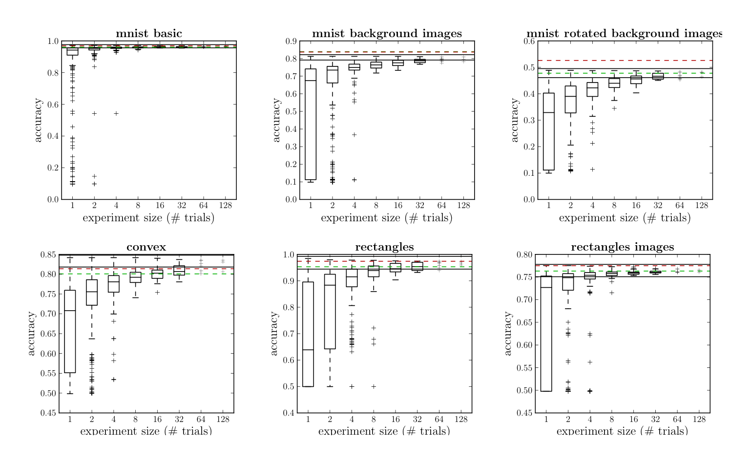
The results of this preliminary random search are in Figure 2. Perhaps surprisingly, the result of manual search can be reliably matched with 32 random trials for several datasets. The efficiency of random search in this setting is explored further in [21]. Where random search results match human performance, it is not clear from Figure 2 whether the reason is that it searched the original space as efficiently, or that it searched a larger space where good performance is easier to find. But the objection that random search is somehow cheating by searching a larger space is backward – the search space outlined in Table 1 is a natural description of the hyper-parameter optimization problem, and the restrictions to that space by [1] were presumably made to simplify the search problem and make it tractable for grid-search assisted manual search. Critically, both methods train DBNs on the same datasets.

The results in Figure 2 indicate that hyper-parameter optimization is harder for some datasets. For example, in the case of the "MNIST rotated background images" dataset (MRBI), random sampling appears to converge to a maximum relatively quickly (best models among experiments of 32 trials show little variance in performance), but this plateau is lower than what was found by manual search. In another dataset (convex), the random sampling procedure exceeds the performance of manual search, but is slow to converge to any sort of plateau. There is considerable variance in generalization when the best of 32 models is selected. This slow convergence indicates that better performance is probably available, but we need to search the configuration space more efficiently to find it. The remainder of this paper explores sequential optimization strategies for hyper-parameter optimization for these two datasets: convex and MRBI.

6 Sequential Search for Hyper-Parameter Optimization in DBNs

Section Summary: The section describes experiments using Gaussian process and tree-structured Parzen estimator models to guide sequential hyper-parameter search for deep belief networks, after first validating the Gaussian process method against plain random sampling on a smaller multilayer perceptron task. Both model-based approaches were initialized with the same thirty random trials and then proposed new configurations for up to two hundred evaluations, with the Parzen estimator proving faster and ultimately finding lower error rates on the convex and MRBI image-classification problems. The searches were executed asynchronously across multiple GPUs by using a temporary “constant liar” value for pending results in the Gaussian process case and by simply ignoring recent proposals in the Parzen estimator case, trading some statistical efficiency for reduced wall-clock time.

We validated our GP approach of Section 3.1 by comparing with random sampling on the Boston Housing dataset, a regression task with 506 points made of 13 scaled input variables and a scalar regressed output. We trained a Multi-Layer Perceptron (MLP) with 10 hyper-parameters, including learning rate, $\ell_1$ and $\ell_2$ penalties, size of hidden layer, number of iterations, whether a PCA pre-processing was to be applied, whose energy was the only conditional hyper-parameter [22]. Our results are depicted in Figure 3. The first 30 iterations were made using random sampling, while from the 30th on, we differentiated the random samples from the GP approach trained on the updated history. The experiment was repeated 20 times. Although the number of points is particularly small compared to the dimensionality, the surrogate modelling approach finds noticeably better points than random, which supports the application of SMBO approaches to more ambitious tasks and datasets.

Applying the GP to the problem of optimizing DBN performance, we allowed 3 random restarts to the CMA+ES algorithm per proposal $x^*$, and up to 500 iterations of conjugate gradient method in fitting the length scales of the GP. The squared exponential kernel [14] was used for every node. The CMA-ES part of GPs dealt with boundaries using a penalty method, the binomial sampling part dealt with it by nature. The GP algorithm was initialized with 30 randomly sampled points in $\mathcal{H}$. After 200 trials, the prediction of a point $x^*$ using this GP took around 150 seconds.

For the TPE-based algorithm, we chose $\gamma = 0.15$ and picked the best among 100 candidates drawn from $\ell(x)$ on each iteration as the proposal $x^*$. After 200 trials, the prediction of a point $x^*$ using this TPE algorithm took around 10 seconds. TPE was allowed to grow past the initial bounds used with for random sampling in the course of optimization, whereas the GP and random search were restricted to stay within the initial bounds throughout the course of optimization. The TPE algorithm was also initialized with the same 30 randomly sampled points as were used to seed the GP.

6.1 Parallelizing Sequential Search

Both the GP and TPE approaches were actually run asynchronously in order to make use of multiple compute nodes and to avoid wasting time waiting for trial evaluations to complete. For the GP approach, the so-called constant liar approach was used: each time a candidate point $x^*$ was proposed, a fake fitness evaluation equal to the mean of the $y

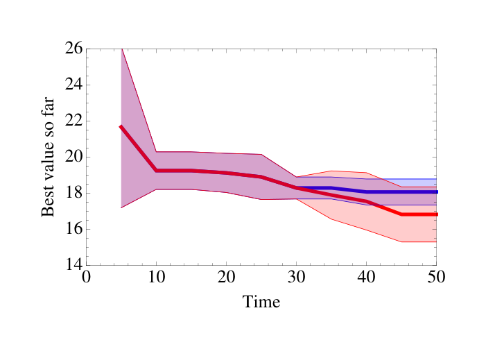
: Table 2: The test set classification error of the best model found by each search algorithm on each problem. Each search algorithm was allowed up to 200 trials. The manual searches used 82 trials for convex and 27 trials MRBI.

\begin{tabular}{lll}
& \textbf{convex} & \textbf{MRBI} \\
\hline
TPE & $\mathbf{14.13 \pm 0.30\,\%}$ & $\mathbf{44.55 \pm 0.44\%}$ \\
GP & $16.70 \pm 0.32\%$ & $47.08 \pm 0.44\%$ \\
Manual & $18.63 \pm 0.34\%$ & $47.39 \pm 0.44\%$ \\
Random & $18.97 \pm 0.34\,\%$ & $50.52 \pm 0.44\%$ \\
\end{tabular}

Runtime per trial was limited to 1 hour of GPU computation regardless of whether execution was on a GTX 285, 470, 480, or 580. The difference in speed between the slowest and fastest machine was roughly two-fold in theory, but the actual efficiency of computation depended also on the load of the machine and the configuration of the problem (the relative speed of the different cards is different in different hyper-parameter configurations). With the parallel evaluation of up to five proposals from the GP and TPE algorithms, each experiment took about 24 hours of wall time using five GPUs.

7 Discussion

Section Summary: The algorithms tested here, especially TPE, produced models that matched or surpassed both random search and careful manual tuning on the two datasets, reaching lower error rates with a comparable number of trials. Several factors may explain TPE’s edge over the Gaussian process approach, such as differences in how each models the relationship between settings and performance, though further experiments would be needed to confirm this. At the same time, these sequential methods can still underperform random search if their internal models are poorly chosen or lead the search toward local rather than global improvements.

The trajectories ($\mathcal{H}$) constructed by each algorithm up to 200 steps are illustrated in Figure 4, and compared with random search and the manual search carried out in [1]. The generalization scores of the best models found using these algorithms and others are listed in Table 2. On the convex dataset (2-way classification), both algorithms converged to a validation score of 13% error. In generalization, TPE's best model had 14.1% error and GP's best had 16.7%. TPE's best was significantly better than both manual search (19%) and random search with 200 trials (17%). On the MRBI dataset (10-way classification), random search was the worst performer (50% error), the GP approach and manual search approximately tied (47% error), while the TPE algorithm found a new best result (44% error). The models found by the TPE algorithm in particular are better than previously found ones on both datasets. The GP and TPE algorithms were slightly less efficient than manual search: GP and EI identified performance on par with manual search within 80 trials, the manual search of [1] used 82 trials for convex and 27 trials for MRBI.

There are several possible reasons for why the TPE approach outperformed the GP approach in these two datasets. Perhaps the inverse factorization of $p(x|y)$ is more accurate than the $p(y|x)$ in the Gaussian process. Perhaps, conversely, the exploration induced by the TPE's lack of accuracy turned out to be a good heuristic for search. Perhaps the hyper-parameters of the GP approach itself were not set to correctly trade off exploitation and exploration in the DBN configuration space. More empirical work is required to test these hypotheses. Critically though, all four SMBO runs matched or exceeded both random search and a careful human-guided search, which are currently the state of the art methods for hyper-parameter optimization.

The GP and TPE algorithms work well in both of these settings, but there are certainly settings in which these algorithms, and in fact SMBO algorithm in general, would not be expected to do well. Sequential optimization algorithms work by leveraging structure in observed $(x, y)$ pairs. It is possible for SMBO to be arbitrarily bad with a bad choice of $p(y|x)$. It is also possible to be slower than random sampling at finding a global optimum with a apparently good $p(y|x)$, if it extracts structure in $\mathcal{H}$ that leads only to a local optimum.

8 Conclusion

Section Summary: This paper presents two algorithms for automatically tuning the many settings of complex machine learning models such as deep belief networks. In tests on two difficult datasets, the methods matched or beat both human experts and simple random searches by exploring a flexible 32-variable space, and they produced new top results in just a day of computation on a few GPUs. The authors argue that such tools make experiments easier to reproduce and allow researchers to study more elaborate models, and they have released one of the algorithms as open-source software.

This paper has introduced two sequential hyper-parameter optimization algorithms, and shown them to meet or exceed human performance and the performance of a brute-force random search in two difficult hyper-parameter optimization tasks involving DBNs. We have relaxed standard constraints (e.g. equal layer sizes at all layers) on the search space, and fall back on a more natural hyper-parameter space of 32 variables (including both discrete and continuous variables) in which many variables are sometimes irrelevant, depending on the value of other parameters (e.g. the number of layers). In this 32-dimensional search problem, the TPE algorithm presented here has uncovered new best results on both of these datasets that are significantly better than what DBNs were previously believed to achieve. Moreover, the GP and TPE algorithms are practical: the optimization for each dataset was done in just 24 hours using five GPU processors. Although our results are only for DBNs, our methods are quite general, and extend naturally to any hyper-parameter optimization problem in which the hyper-parameters are drawn from a measurable set.

We hope that our work may spur researchers in the machine learning community to treat the hyper-parameter optimization strategy as an interesting and important component of all learning algorithms. The question of "How well does a DBN do on the convex task?" is not a fully specified, empirically answerable question – different approaches to hyper-parameter optimization will give different answers. Algorithmic approaches to hyper-parameter optimization make machine learning results easier to disseminate, reproduce, and transfer to other domains. The specific algorithms we have presented here are also capable, at least in some cases, of finding better results than were previously known. Finally, powerful hyper-parameter optimization algorithms broaden the horizon of models that can realistically be studied; researchers need not restrict themselves to systems of a few variables that can readily be tuned by hand.

The TPE algorithm presented in this work, as well as parallel evaluation infrastructure, is available as BSD-licensed free open-source software, which has been designed not only to reproduce the results in this work, but also to facilitate the application of these and similar algorithms to other hyper-parameter optimization problems.[^1]

[^1]: "Hyperopt" software package: https://github.com/jaberg/hyperopt

Acknowledgements

This work was supported by the National Science and Engineering Research Council of Canada, Compute Canada, and by the ANR-2010-COSI-002 grant of the French National Research Agency. GPU implementations of the DBN model were provided by Theano [23].

References

Section Summary: This section consists of a numbered bibliography with 23 entries, primarily academic papers and a few books or theses on machine learning topics. The references cover areas such as deep neural networks, unsupervised feature learning, algorithm configuration and optimization methods like Gaussian processes, and supporting tools for scientific computing. They span publications from the late 1990s through 2012, drawing from conferences like ICML and NIPS as well as journals in the field.

[1] H. Larochelle, D. Erhan, A. Courville, J. Bergstra, and Y. Bengio. An empirical evaluation of deep architectures on problems with many factors of variation. In ICML 2007, pages 473–480, 2007.

[2] G. E. Hinton, S. Osindero, and Y. Teh. A fast learning algorithm for deep belief nets. Neural Computation, 18:1527–1554, 2006.

[3] P. Vincent, H. Larochelle, I. Lajoie, Y. Bengio, and P. A. Manzagol. Stacked denoising autoencoders: Learning useful representations in a deep network with a local denoising criterion. Machine Learning Research, 11:3371–3408, 2010.

[4] Y. LeCun, L. Bottou, Y. Bengio, and P. Haffner. Gradient-based learning applied to document recognition. Proceedings of the IEEE, 86(11):2278–2324, November 1998.

[5] Nicolas Pinto, David Doukhan, James J. DiCarlo, and David D. Cox. A high-throughput screening approach to discovering good forms of biologically inspired visual representation. PLoS Comput Biol, 5(11):e1000579, 11 2009.

[6] A. Coates, H. Lee, and A. Ng. An analysis of single-layer networks in unsupervised feature learning. NIPS Deep Learning and Unsupervised Feature Learning Workshop, 2010.

[7] A. Coates and A. Y. Ng. The importance of encoding versus training with sparse coding and vector quantization. In Proceedings of the Twenty-eighth International Conference on Machine Learning (ICML-11), 2010.

[8] F. Hutter. Automated Configuration of Algorithms for Solving Hard Computational Problems. PhD thesis, University of British Columbia, 2009.

[9] F. Hutter, H. Hoos, and K. Leyton-Brown. Sequential model-based optimization for general algorithm configuration. In LION-5, 2011. Extended version as UBC Tech report TR-2010-10.

[10] D.R. Jones. A taxonomy of global optimization methods based on response surfaces. Journal of Global Optimization, 21:345–383, 2001.

[11] J. Villemonteix, E. Vazquez, and E. Walter. An informational approach to the global optimization of expensive-to-evaluate functions. Journal of Global Optimization, 2006.

[12] N. Srinivas, A. Krause, S. Kakade, and M. Seeger. Gaussian process optimization in the bandit setting: No regret and experimental design. In ICML, 2010.

[13] J. Mockus, V. Tiesis, and A. Zilinskas. The application of Bayesian methods for seeking the extremum. In L.C.W. Dixon and G.P. Szego, editors, Towards Global Optimization, volume 2, pages 117–129. North Holland, New York, 1978.

[14] C.E. Rasmussen and C. Williams. Gaussian Processes for Machine Learning.

[15] D. Ginsbourger, D. Dupuy, A. Badea, L. Carraro, and O. Roustant. A note on the choice and the estimation of kriging models for the analysis of deterministic computer experiments. 25:115–131, 2009.

[16] R. Bardenet and B. Kégl. Surrogating the surrogate: accelerating Gaussian Process optimization with mixtures. In ICML, 2010.

[17] P. Larrañaga and J. Lozano, editors. Estimation of Distribution Algorithms: A New Tool for Evolutionary Computation. Springer, 2001.

[18] N. Hansen. The CMA evolution strategy: a comparing review. In J.A. Lozano, P. Larrañaga, I. Inza, and E. Bengoetxea, editors, Towards a new evolutionary computation. Advances on estimation of distribution algorithms, pages 75–102. Springer, 2006.

[19] J. Bergstra and Y. Bengio. Random search for hyper-parameter optimization. The Learning Workshop (Snowbird), 2011.

[20] A. Hyvärinen and E. Oja. Independent component analysis: Algorithms and applications. Neural Networks, 13(4–5):411–430, 2000.

[21] J. Bergstra and Y. Bengio. Random search for hyper-parameter optimization. JMLR, 2012. Accepted.

[22] C. Bishop. Neural networks for pattern recognition. 1995.

[23] J. Bergstra, O. Breuleux, F. Bastien, P. Lamblin, R. Pascanu, G. Desjardins, J. Turian, and Y. Bengio. Theano: a CPU and GPU math expression compiler. In Proceedings of the Python for Scientific Computing Conference (SciPy), June 2010.