An Introduction to the Kalman Filter

Greg WelchGary Bishop

article1995University of North Carolina at Chapel Hill Technical Report 95-0416,252 citations

Explains the mechanics of discrete and extended Kalman filters by pairing accessible mathematical derivations with a concrete, step-by-step numerical example.

Listen

The document introduces the Kalman filter as a practical computational tool for estimating the state of a process from noisy measurements. First published in 1960, the method gained wide use in navigation and control once digital computers made recursive calculations routine. The core challenge it addresses is estimating unknown quantities in real time when only incomplete or noisy observations are available and when running a full batch solution on all past data is impractical.

The authors set out to supply a clear, self-contained derivation and explanation of the basic discrete Kalman filter, its extension to nonlinear problems, and a worked numerical example that shows how the equations behave.

They derive the filter from the goal of minimizing posterior error covariance, present the resulting time-update and measurement-update equations in matrix form, and illustrate their use on a simple scalar problem of estimating a fixed random voltage from fifty noisy readings. The same structure is then generalized to the extended Kalman filter by linearizing the process and measurement models with Jacobian matrices at each step.

The analysis shows that the filter converges reliably once the measurement-noise covariance R is known and the process-noise covariance Q is chosen to reflect model uncertainty. In the example, setting R to its true value produced an estimate whose variance settled near 0.0002 after fifty steps; increasing R by a factor of one hundred slowed response and reduced estimate variance, while decreasing R had the opposite effect. The extended form preserves the same predictor-corrector cycle but approximates optimality through local linearization.

These results matter because the recursive structure allows real-time state estimation on modest hardware without storing or reprocessing all prior data, a decisive advantage for autonomous navigation, tracking, and sensor fusion. Proper tuning of Q and R directly trades off tracking speed against smoothness, giving designers explicit control over performance.

The paper recommends measuring R from off-line samples of the sensor, selecting Q to inject realistic process uncertainty, and, when dynamics change, allowing Q to vary during operation. For strongly nonlinear problems the extended filter remains usable, yet users should verify observability; divergence occurs quickly if measurements do not adequately constrain the state. Further work is advisable to test the filter on the target hardware with actual sensor statistics before deployment.

The derivations rest on assumptions of Gaussian white noise and either linear or locally linear models. The single scalar example is deliberately simple; performance on higher-dimensional or poorly observable systems is not demonstrated. The authors note that the extended filter is an approximation whose error statistics are no longer exactly Gaussian after nonlinear transformations.

University of North Carolina at Chapel Hill real number filtering problems efficient computation Kalman filter extended Kalman filter discrete Kalman filter

Welch et al (1995).pdf

Book: Introduction to Probability, Charles M. Grinstead et al. (1997). Mastering the rules of probability and random variables from this textbook is essential for understanding the stochastic noise models underpinning the discrete Kalman filter.
Book: Mathematics for Machine Learning, Garrett Thomas. A firm grasp of matrix operations, orthogonal projections, and linear transformations from this linear algebra review is required to follow the algebraic derivations of the Kalman update equations.

No sufficiently relevant recommendations were found.

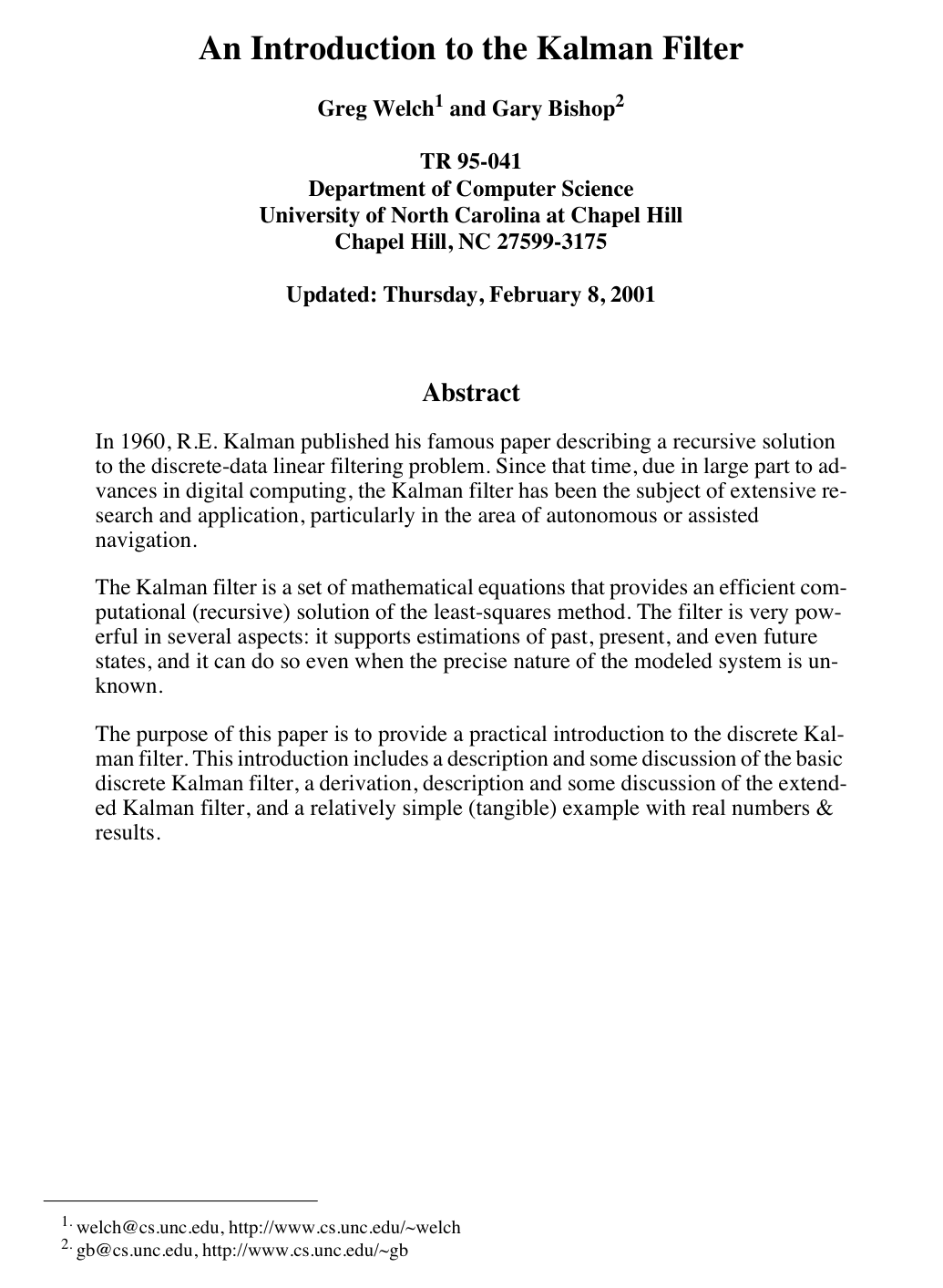
Cover for An Introduction to the Kalman Filter

Abstract

In 1960, R.E. Kalman published his famous paper describing a recursive solution to the discrete-data linear filtering problem. Since that time, due in large part to advances in digital computing, the Kalman filter has been the subject of extensive research and application, particularly in the area of autonomous or assisted navigation.

The Kalman filter is a set of mathematical equations that provides an efficient computational (recursive) solution of the least-squares method. The filter is very powerful in several aspects: it supports estimations of past, present, and even future states, and it can do so even when the precise nature of the modeled system is unknown.

The purpose of this paper is to provide a practical introduction to the discrete Kalman filter. This introduction includes a description and some discussion of the basic discrete Kalman filter, a derivation, description and some discussion of the extended Kalman filter, and a relatively simple (tangible) example with real numbers & results.

Topics

real number filtering problems efficient computation unscented kalman filter

Keywords

Kalman filter extended Kalman filter discrete Kalman filter Kalman gain linear filtering measurement update equations measurement noise covariance optimal estimation stochastic difference equation estimate error covariance

1 The Discrete Kalman Filter
*The Process to be Estimated*
*The Computational Origins of the Filter*
*The Probabilistic Origins of the Filter*
*The Discrete Kalman Filter Algorithm*
Filter Parameters and Tuning
2 The Extended Kalman Filter (EKF)
*The Process to be Estimated*
The Computational Origins of the Filter
3 A Kalman Filter in Action: Estimating a Random Constant
*The Process Model*
The Filter Equations and Parameters
*The Simulations*
References

Knowls

Knowl 1 — Discrete Kalman Filter Predict-Correct Algorithm
algorithm
The discrete Kalman filter maintains the conditional mean $\hat{x}_k$ (state estimate) and error covariance $P_k = \mathbb{E}[(x_k - \hat{x}_k)(x_k - \hat{x}_k)^T]$ through alternating time update (prediction) and measurement update (correction) steps.
Input: Initial state estimate $\hat{x}_0$ , initial error covariance $P_0$ , process model matrices $A$ and $B$ , control inputs $u_k$ , process noise covariance $Q$ , measurement matrix $H$ , measurement noise covariance $R$ , sequence of measurements $z_k$ for $k = 1, 2, \dots$
Output: A posteriori state estimates $\hat{x}_k$ and error covariances $P_k$ for each step $k$
for $k = 1, 2, \dots$ do
    Time Update (Predict):
         $\hat{x}_k^- = A \hat{x}_{k-1} + B u_k$
         $P_k^- = A P_{k-1} A^T + Q$
    Measurement Update (Correct):
         $K_k = P_k^- H^T (H P_k^- H^T + R)^{-1}$
         $\hat{x}_k = \hat{x}_k^- + K_k (z_k - H \hat{x}_k^-)$
         $P_k = (I - K_k H) P_k^-$
    return $\hat{x}_k, P_k$
Here, $\hat{x}_k^-$ and $P_k^-$ denote the a priori state estimate and error covariance at step $k$ prior to incorporating measurement $z_k$ ; $K_k \in \mathbb{R}^{n \times m}$ is the Kalman gain; $z_k - H \hat{x}_k^-$ is the measurement innovation (residual); and $I$ is the $n \times n$ identity matrix.
Knowl 2 — Discrete Linear Process and Measurement System Model
model/method
The discrete linear Kalman filter estimates an $n$ -dimensional state vector $x_k \in \mathbb{R}^n$ at discrete time step $k$ governed by a linear stochastic difference equation with measurement $z_k \in \mathbb{R}^m$ :

$x_k = A x_{k-1} + B u_k + w_{k-1}$

$z_k = H x_k + v_k$

where:
- $A$ is an $n \times n$ state transition matrix relating the state at step $k-1$ to the state at step $k$ in the absence of control input or process noise.
- $B$ is an $n \times l$ control-input matrix relating the optional control vector $u_k \in \mathbb{R}^l$ to the state $x_k$ .
- $H$ is an $m \times n$ measurement matrix relating the state $x_k$ to the measurement $z_k$ .
- $w_k \in \mathbb{R}^n$ is the process noise vector, assumed to be white, zero-mean Gaussian noise with covariance matrix $Q \in \mathbb{R}^{n \times n}$ , i.e., $p(w) \sim \mathcal{N}(0, Q)$ .
- $v_k \in \mathbb{R}^m$ is the measurement noise vector, assumed to be white, zero-mean Gaussian noise with covariance matrix $R \in \mathbb{R}^{m \times m}$ , i.e., $p(v) \sim \mathcal{N}(0, R)$ .
- The random noise vectors $w_k$ and $v_k$ are assumed mutually independent.
Knowl 3 — Extended Kalman Filter Estimation Algorithm
algorithm
The Extended Kalman Filter (EKF) approximates optimal non-linear state estimation by linearizing non-linear process dynamics $f$ and measurement functions $h$ around the current state estimates at each time step.
Input: Initial state estimate $\hat{x}_0$ , initial error covariance $P_0$ , non-linear state transition function $f$ , non-linear measurement function $h$ , control inputs $u_k$ , process noise covariance $Q_k$ , measurement noise covariance $R_k$ , sequence of measurements $z_k$ for $k = 1, 2, \dots$
Output: A posteriori state estimates $\hat{x}_k$ and error covariances $P_k$ for each step $k$
for $k = 1, 2, \dots$ do
    Time Update (Predict):
         $\hat{x}_k^- = f(\hat{x}_{k-1}, u_k, 0)$
        Compute Jacobians $A_k = \frac{\partial f}{\partial x}(\hat{x}_{k-1}, u_k, 0)$ and $W_k = \frac{\partial f}{\partial w}(\hat{x}_{k-1}, u_k, 0)$
         $P_k^- = A_k P_{k-1} A_k^T + W_k Q_{k-1} W_k^T$
    Measurement Update (Correct):
        Compute Jacobians $H_k = \frac{\partial h}{\partial x}(\hat{x}_k^-, 0)$ and $V_k = \frac{\partial h}{\partial v}(\hat{x}_k^-, 0)$
         $K_k = P_k^- H_k^T (H_k P_k^- H_k^T + V_k R_k V_k^T)^{-1}$
         $\hat{x}_k = \hat{x}_k^- + K_k (z_k - h(\hat{x}_k^-, 0))$
         $P_k = (I - K_k H_k) P_k^-$
    return $\hat{x}_k, P_k$
Here, $\hat{x}_k^-$ and $P_k^-$ denote the a priori state estimate and error covariance; $K_k$ is the Kalman gain; $z_k - h(\hat{x}_k^-, 0)$ is the non-linear measurement residual; and $I$ is the identity matrix.
Knowl 4 — Non-linear System Formulation and Linearization for the Extended Kalman Filter
model/method
When a discrete-time controlled process or its measurement relationship is non-linear, the process is governed by non-linear stochastic difference equations:

$x_k = f(x_{k-1}, u_k, w_{k-1})$

$z_k = h(x_k, v_k)$

where $x_k \in \mathbb{R}^n$ is the state vector, $z_k \in \mathbb{R}^m$ is the measurement vector, $u_k \in \mathbb{R}^l$ is the control input, $w_k \sim \mathcal{N}(0, Q_k)$ is zero-mean process noise, and $v_k \sim \mathcal{N}(0, R_k)$ is zero-mean measurement noise.

Linearization is performed around the current estimates using first-order Taylor approximations via Jacobian matrices:

$A_{k[i, j]} = \frac{\partial f_{[i]}}{\partial x_{[j]}}(\hat{x}_{k-1}, u_k, 0)$

$W_{k[i, j]} = \frac{\partial f_{[i]}}{\partial w_{[j]}}(\hat{x}_{k-1}, u_k, 0)$

$H_{k[i, j]} = \frac{\partial h_{[i]}}{\partial x_{[j]}}(\hat{x}_k^-, 0)$

$V_{k[i, j]} = \frac{\partial h_{[i]}}{\partial v_{[j]}}(\hat{x}_k^-, 0)$

where $\hat{x}_{k-1}$ is the a posteriori state estimate from step $k-1$ , and $\hat{x}_k^- = f(\hat{x}_{k-1}, u_k, 0)$ is the a priori state estimate at step $k$ evaluated with zero process noise.
Knowl 5 — Asymptotic Behavior of the Kalman Gain with Error Covariances
theoretical result
The Kalman gain $K_k$ at time step $k$ is given by:

$K_k = P_k^- H^T (H P_k^- H^T + R)^{-1}$

where $P_k^-$ is the a priori state error covariance matrix, $H$ is the measurement matrix, and $R$ is the measurement noise covariance matrix.

The gain balances reliance between the model prediction and the measurement innovation with the following limiting behaviors:
- As the measurement error covariance approaches zero ( $R \to 0$ ), the Kalman gain satisfies:
$\lim_{R \to 0} K_k = H^{-1}$

(assuming $H$ is invertible), meaning the filter places full weight on the actual measurement $z_k$ and ignores the predicted measurement $H \hat{x}_k^-$ .
- As the a priori estimate error covariance approaches zero ( $P_k^- \to 0$ ), the Kalman gain satisfies:
$\lim_{P_k^- \to 0} K_k = 0$

meaning the filter places zero weight on the measurement innovation and relies completely on the time update model prediction.
Knowl 6 — Non-Gaussian Distribution Distortion in Extended Kalman Filtering
limitation
A fundamental limitation of the Extended Kalman Filter (EKF) is that probability distributions (or probability density functions) of random state variables no longer remain Gaussian (normal) after undergoing non-linear transformations $f(\cdot)$ and $h(\cdot)$ .

Consequently, the EKF is an ad hoc state estimator that only approximates the optimal Bayesian conditional probability update via first-order Taylor series linearization. If the system is highly non-linear or if there is no one-to-one mapping between measurement $z_k$ and state $x_k$ via $h$ across measurements (making the process unobservable), the filter may rapidly diverge.
Knowl 7 — Experimental Setup for Scalar Random Constant Estimation
experimental setup
A discrete Kalman filter is evaluated on estimating a scalar constant voltage $x_k \in \mathbb{R}$ governed by:

$x_k = x_{k-1} + w_k$

$z_k = x_k + v_k$

with constant scalar parameters $A = 1$ , control input $u = 0$ , measurement relation $H = 1$ , and process noise covariance $Q = 10^{-5}$ .

The true scalar constant is fixed to $x = -0.37727\text{ V}$ . A sequence of 50 discrete measurements $z_k$ is simulated by corrupting the true value with zero-mean white Gaussian noise with standard deviation $\sigma_v = 0.1\text{ V}$ (true measurement variance $R = \sigma_v^2 = 0.01\text{ V}^2$ ). The filter is initialized with prior state estimate guess $\hat{x}_0 = 0\text{ V}$ and initial error covariance $P_0 = 1\text{ V}^2$ .
Knowl 8 — Convergence and Responsiveness Under Varying Measurement Noise Covariance
empirical result
In the 50-iteration scalar constant estimation simulation ( $x = -0.37727\text{ V}$ , true noise variance $R_{\text{true}} = 0.01\text{ V}^2$ , $Q = 10^{-5}$ , initial estimate $\hat{x}_0 = 0$ , $P_0 = 1$ ):
1. Nominal Tuning ( $R = 0.01$ ): With the filter configured with the true measurement error variance $R = 0.01\text{ V}^2$ , the error covariance $P_k$ converges monotonically from $P_0 = 1$ to approximately $0.0002\text{ V}^2$ by the 50th iteration, achieving a balanced trade-off between responsiveness to measurements and estimate variance reduction.
2. High Measurement Covariance ( $R = 1$ ): When the filter is parameterized with $R = 1\text{ V}^2$ (100 times larger than the true variance), the filter trusts incoming measurements significantly less, yielding a slower response and a smoother estimate curve with lower estimate variance.
3. Low Measurement Covariance ( $R = 0.0001$ ): When parameterized with $R = 0.0001\text{ V}^2$ (100 times smaller than the true variance), the filter rapidly incorporates noisy measurements, resulting in high responsiveness but substantially increased estimate variance.

Coverage note — No substantial contributed material was omitted; the tutorial's foundational derivations, discrete linear formulation, extended non-linear formulation, limitations, and empirical constant estimation experiment are fully represented.

References

1.Brown, R. G. and P. Y. C. Hwang. 1992. Introduction to Random Signals and Applied Kalman Filtering, Second Edition, John Wiley & Sons, Inc.
2.Gelb, A. 1974. Applied Optimal Estimation, MIT Press, Cambridge, MA.
3.Grewal, Mohinder S., and Angus P. Andrews (1993). Kalman Filtering Theory and Practice. Upper Saddle River, NJ USA, Prentice Hall.
4.Jacobs, O. L. R. 1993. Introduction to Control Theory, 2nd Edition. Oxford University Press.
5.Julier, Simon and Jeffrey Uhlman. “A General Method of Approximating Nonlinear Transformations of Probability Distributions,” Robotics Research Group, Department of Engineering Science, University of Oxford [cited 14 November 1995]. Available from http://www.robots.ox.ac.uk/~siju/work/publications/Unscented.zip. Also see: “A New Approach for Filtering Nonlinear Systems” by S. J. Julier, J. K. Uhlmann, and H. F. Durrant-Whyte, Proceedings of the 1995 American Control Conference, Seattle, Washington, Pages:1628-1632. Available from http://www.robots.ox.ac.uk/~siju/work/publications/ACC95_pr.zip. Also see Simon Julier's home page at http://www.robots.ox.ac.uk/~siju/.
6.Kalman, R. E. 1960. “A New Approach to Linear Filtering and Prediction Problems,” Transaction of the ASME—Journal of Basic Engineering, pp. 35-45 (March 1960).
7.Lewis, Richard. 1986. Optimal Estimation with an Introduction to Stochastic Control Theory, John Wiley & Sons, Inc.
8.Maybeck, Peter S. 1979. Stochastic Models, Estimation, and Control, Volume 1, Academic Press, Inc.
9.Sorenson, H. W. 1970. “Least-Squares estimation: from Gauss to Kalman,” IEEE Spectrum, vol. 7, pp. 63-68, July 1970.

Citation

MLA

Welch, G., and G. Bishop. An Introduction to the Kalman Filter. CiteSeer X (The Pennsylvania State University), vol. 1, no. 4, 1995, pp. 1–6, http://citeseerx.ist.psu.edu/viewdoc/summary?doi=10.1.1.705.3475.

APA

Welch, G., & Bishop, G. (1995). An Introduction to the Kalman Filter. In CiteSeer X (The Pennsylvania State University) (Vol. 1, Issue 4, pp. 1–16). http://citeseerx.ist.psu.edu/viewdoc/summary?doi=10.1.1.705.3475

Chicago

Welch, G., and G. Bishop. 1995. An Introduction to the Kalman Filter. In CiteSeer X (The Pennsylvania State University), vol. 1. no. 4. http://citeseerx.ist.psu.edu/viewdoc/summary?doi=10.1.1.705.3475.

Harvard

Welch, G. and Bishop, G. (1995) An Introduction to the Kalman Filter, CiteSeer X (The Pennsylvania State University), pp. 1–16. Available at: http://citeseerx.ist.psu.edu/viewdoc/summary?doi=10.1.1.705.3475.

Vancouver

1. Welch G, Bishop G (1995) An Introduction to the Kalman Filter. CiteSeer X (The Pennsylvania State University) 1:1–16

BibTeX

@book{welch1995introduction,
  title = {An Introduction to the Kalman Filter},
  author = {Welch, Greg and Bishop, Gary},
  year = {1995},
  booktitle = {CiteSeer X (The Pennsylvania State University)},
  volume = {1},
  number = {4},
  pages = {1-16},
  url = {http://citeseerx.ist.psu.edu/viewdoc/summary?doi=10.1.1.705.3475}
}

Metadata:DOI registry

Access the Paper

This paper is available from its original source. Click below to access the PDF.

Open PDF

An Introduction to the Kalman Filter

Abstract

Topics

Keywords

Table of Contents

Knowls

Knowl 1 — Discrete Kalman Filter Predict-Correct Algorithm

Knowl 2 — Discrete Linear Process and Measurement System Model

Knowl 3 — Extended Kalman Filter Estimation Algorithm

Knowl 4 — Non-linear System Formulation and Linearization for the Extended Kalman Filter

Knowl 5 — Asymptotic Behavior of the Kalman Gain with Error Covariances

Knowl 6 — Non-Gaussian Distribution Distortion in Extended Kalman Filtering

Knowl 7 — Experimental Setup for Scalar Random Constant Estimation

Knowl 8 — Convergence and Responsiveness Under Varying Measurement Noise Covariance

References

Citation

BibTeX

Access the Paper