FlowNet 2.0: Evolution of Optical Flow Estimation with Deep Networks

Eddy IlgNikolaus MayerTonmoy SaikiaMargret KeuperAlexey DosovitskiyThomas Brox

article2016CVPR3,421 citations

Introduces a stacked deep learning architecture that integrates intermediate image warping, small-motion sub-networks, and phased training schedules, cutting optical flow estimation error by more than 50% while achieving real-time speeds up to 140 frames per second.

Listen

The paper introduces FlowNet 2.0, a family of convolutional networks that substantially advances end-to-end learning for optical flow estimation. Earlier work had shown that optical flow could be cast as a supervised learning problem, yet the original FlowNet still trailed classical variational methods, especially on small displacements and real-world video. The authors set out to close that gap while preserving the speed advantage of feed-forward networks.

They addressed the problem through three coordinated changes: a curriculum-style training schedule that first uses a simple synthetic dataset of flying chairs and then fine-tunes on a more realistic three-dimensional dataset; repeated stacking of networks that warp the second image by the current flow estimate before feeding it forward; and a specialized sub-network, together with a small fusion stage, that focuses on sub-pixel motion. All variants were trained on publicly released synthetic data and evaluated on the standard Sintel, KITTI, and Middlebury benchmarks as well as on downstream tasks such as motion segmentation and action recognition.

The resulting networks cut endpoint error by more than half relative to the original FlowNet while remaining only marginally slower. The best configuration matches or exceeds the accuracy of the leading variational methods on Sintel and KITTI yet runs at 8–140 frames per second on a single GPU, depending on the chosen width and depth. Performance on real video improves markedly, producing smoother fields, sharper motion boundaries, and greater robustness to compression artifacts and homogeneous regions. On motion segmentation and action recognition the learned flow yields results comparable to the best traditional methods while operating orders of magnitude faster.

These gains demonstrate that carefully scheduled supervised training and iterative refinement inside a feed-forward architecture can replace expensive optimization loops without sacrificing accuracy. Practitioners can therefore select a speed–accuracy operating point from the FlowNet 2.0 family for real-time applications that previously required offline processing. Further gains will most likely come from domain-specific fine-tuning on target video distributions and from modest architectural adjustments that reduce residual noise on very small motions. The main remaining uncertainty is how well the networks generalize to entirely novel scene types not represented in the current synthetic training mixtures; additional labeled real-world data would reduce that risk.

University of Freiburg optical flow computation optical flow estimation variational methods optical flow estimation FlowNet architecture large displacement optical flow

arXiv: 1612.01925 lmb-freiburg/flownet2

Paper: FlowNet: Learning Optical Flow with Convolutional Networks, Philipp Fischer et al. (2015). FlowNet established the foundational deep learning framework and synthetic datasets for end-to-end optical flow estimation that FlowNet 2.0 directly builds upon and refines.

Paper: RAFT: Recurrent All-Pairs Field Transforms for Optical Flow, Zachary Teed et al. (2020). RAFT continues the evolution of deep learning for optical flow by replacing stacked warping architectures with recurrent all-pairs field transforms for superior accuracy and generalization.

Cover for FlowNet 2.0: Evolution of Optical Flow Estimation with Deep Networks

Abstract

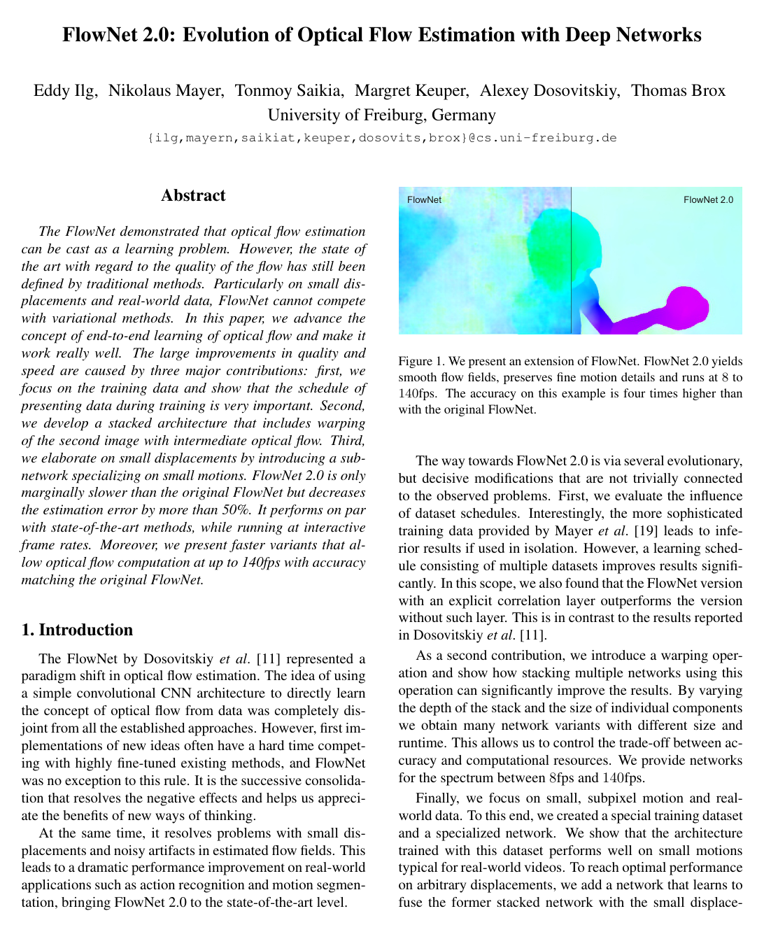
The FlowNet demonstrated that optical flow estimation can be cast as a learning problem. However, the state of the art with regard to the quality of the flow has still been defined by traditional methods. Particularly on small displacements and real-world data, FlowNet cannot compete with variational methods. In this paper, we advance the concept of end-to-end learning of optical flow and make it work really well. The large improvements in quality and speed are caused by three major contributions: first, we focus on the training data and show that the schedule of presenting data during training is very important. Second, we develop a stacked architecture that includes warping of the second image with intermediate optical flow. Third, we elaborate on small displacements by introducing a sub-network specializing on small motions. FlowNet 2.0 is only marginally slower than the original FlowNet but decreases the estimation error by more than 50%. It performs on par with state-of-the-art methods, while running at interactive frame rates. Moreover, we present faster variants that allow optical flow computation at up to 140fps with accuracy matching the original FlowNet.

Topics

optical flow computation optical flow estimation variational methods estimation method optical flow algorithm network architecture optical flow methods stereo matching

Keywords

optical flow estimation FlowNet architecture large displacement optical flow iterative flow field refinement deep matching motion estimation fusion network motion segmentation

1. Introduction
2. Related Work
3. Dataset Schedules
4. Stacking Networks
4.1. Stacking Two Networks for Flow Refinement
4.2. Stacking Multiple Diverse Networks
5. Small Displacements
5.1. Datasets
5.2. Small Displacement Network and Fusion
6. Experiments
6.1. Speed and Performance on Public Benchmarks
6.2. Qualitative Results
6.3. Performance on Motion Segmentation and Action Recognition
7. Conclusions
Acknowledgements
References
1. Video
2. Dataset Schedules: KITTI2015 Results
3. Recurrently Stacking Networks with the Same Weights
4. Small Displacements
4.1. The ChairsSDHom Dataset
4.2. Fine-Tuning FlowNet2-CSS-ft-sd
4.3. Network Architectures
5. Evaluation
5.1. Intermediate Results in Stacked Networks
5.2. Speed and Performance on KITTI2012
5.3. Motion Segmentation
5.4. Qualitative results on KITTI2015
6. Warping Layer
6.1. Definitions and Bilinear Interpolation
6.2. Forward Pass
6.3. Backward Pass

Knowls

Knowl 1 — FlowNet 2.0 Overall Architecture and Fusion Pipeline
model/method
The FlowNet 2.0 architecture integrates deep learning pipelines specialized for both large and small displacement regimes through a learned fusion mechanism:
1. Large Displacement Branch (FlowNet2-CSS-ft-sd): Consists of a three-network cascade (one FlowNetC feature correlation network followed by two FlowNetS encoder-decoder networks). Each subsequent network receives the first image $I_1$ , the second image $I_2$ , the previous flow estimate $\mathbf{w}_i = (u_i, v_i)^\top$ , the warped second image $\tilde{I}_{2,i}$ , and the absolute brightness error $e_i = \|\tilde{I}_{2,i} - I_1\|$ . This stack is fine-tuned on a combination of FlyingThings3D and ChairsSDHom data with down-weighted large displacements to preserve large-motion handling while improving small-motion accuracy.
2. Small Displacement Branch (FlowNet2-SD): A modified FlowNetS architecture specialized for subpixel motions and smooth flow fields. It processes concatenated input images $(I_1, I_2)$ with stride-1 convolutions at the initial layer, deeper initial layers composed of $3\times 3$ kernels instead of $7\times 7$ and $5\times 5$ kernels, and additional convolution layers interleaved between upconvolutions.
3. Fusion Network: Merges the flow predictions from the large displacement branch and the small displacement branch. It takes an 11-channel input at full image resolution consisting of:
  - The reference image $I_1$ (3 channels),
  - The flow estimate from FlowNet2-CSS-ft-sd (2 channels),
  - The flow estimate from FlowNet2-SD (2 channels),
  - The magnitudes of both flow estimates (2 channels),
  - The per-pixel squared Euclidean photoconsistency errors $\|\tilde{I}_{2} - I_1\|^2$ for both flow fields (2 channels).
The fusion network contracts the spatial resolution by a factor of 4 via two stride-2 pooling/convolution stages and expands back with skip connections to the full image resolution, producing crisp motion boundaries and selecting the appropriate flow regime per pixel.
Knowl 2 — Iterative Flow Refinement via Network Stacking with Warping
model/method
Optical flow estimation accuracy is refined by stacking multiple convolutional networks sequentially. Rather than computing optical flow in a single pass, subsequent networks compute residual corrections to an initial estimate.

Let $I_1, I_2: \Omega \to \mathbb{R}^3$ be a pair of input images on the pixel domain $\Omega \subset \mathbb{R}^2$ . The first network in the stack predicts an initial flow field $\mathbf{w}_1 = (u_1, v_1)^\top$ . For any subsequent stage $i+1$ , the second image $I_2$ is warped according to the current cumulative flow estimate $\mathbf{w}_i$ via bilinear interpolation: $\tilde{I}_{2,i}(\mathbf{x}) = I_2(\mathbf{x} + \mathbf{w}_i(\mathbf{x}))$

The $(i+1)$ -th network is provided with a concatenated multi-channel input composed of:
- The reference image $I_1$ ,
- The original target image $I_2$ ,
- The current flow estimate $\mathbf{w}_i$ ,
- The warped target image $\tilde{I}_{2,i}$ ,
- The absolute brightness error map $e_i(\mathbf{x}) = \|\tilde{I}_{2,i}(\mathbf{x}) - I_1(\mathbf{x})\|$ .
To prevent the stacked model from overfitting to the training distribution, the stack is trained sequentially (step-by-step): the parameters of stage $1, \dots, i$ are kept fixed while training stage $i+1$ . Stacking networks with warping consistently improves endpoint error across benchmarks, whereas stacking networks without warping degrades cross-dataset generalization.
Knowl 3 — Differentiable Image Warping Layer and Analytical Gradients
equation
Let $I: \mathbb{R}^2 \to \mathbb{R}^C$ be an image or feature map with $C$ channels defined on integer grid coordinates $\mathcal{R} \subset \mathbb{Z}^2$ , and let $\mathbf{w}(\mathbf{x}) = (u(\mathbf{x}), v(\mathbf{x}))^\top$ denote a continuous 2D flow field at pixel location $\mathbf{x} = (x, y)^\top$ .

Define subpixel offset coefficients: $\theta_x = x - \lfloor x \rfloor, \quad \bar{\theta}_x = 1 - \theta_x, \quad \theta_y = y - \lfloor y \rfloor, \quad \bar{\theta}_y = 1 - \theta_y$

The continuous bilinearly interpolated image $\tilde{I}(\mathbf{x})$ is defined as: $\tilde{I}(x, y) = \bar{\theta}_x \bar{\theta}_y I(\lfloor x \rfloor, \lfloor y \rfloor) + \theta_x \bar{\theta}_y I(\lceil x \rceil, \lfloor y \rfloor) + \bar{\theta}_x \theta_y I(\lfloor x \rfloor, \lceil y \rceil) + \theta_x \theta_y I(\lceil x \rceil, \lceil y \rceil)$

The forward warping operation $J_{I, \mathbf{w}}(\mathbf{x})$ evaluates $\tilde{I}$ at target coordinates $(p, q)^\top = \mathbf{x} + \mathbf{w}(\mathbf{x})$ : $J_{I, \mathbf{w}}(\mathbf{x}) = \begin{cases} \tilde{I}(\mathbf{x} + \mathbf{w}(\mathbf{x})) & \text{if } \mathbf{x} + \mathbf{w}(\mathbf{x}) \in \mathcal{R} \\ 0 & \text{otherwise} \end{cases}$

During backpropagation, the derivative of channel $c$ of the warped output $J_c(\mathbf{x})$ with respect to the input intensity $I_c(\mathbf{x}')$ at integer location $\mathbf{x}' = (x', y')^\top$ is: $\frac{\partial J_c(\mathbf{x})}{\partial I_c(\mathbf{x}')} = \bar{\theta}_p \bar{\theta}_q \delta(\lfloor p \rfloor = x')\delta(\lfloor q \rfloor = y') + \theta_p \bar{\theta}_q \delta(\lceil p \rceil = x')\delta(\lfloor q \rfloor = y') + \bar{\theta}_p \theta_q \delta(\lfloor p \rfloor = x')\delta(\lceil q \rceil = y') + \theta_p \theta_q \delta(\lceil p \rceil = x')\delta(\lceil q \rceil = y')$ where $\delta(\cdot)$ is the indicator function ( $\{0, 1\}$ ).

The derivative of the warped image with respect to the horizontal displacement component $u(\mathbf{x}')$ is non-zero only when $\mathbf{x} = \mathbf{x}'$ and $(p, q)^\top \in \mathcal{R}$ : $\frac{\partial J(\mathbf{x})}{\partial u(\mathbf{x}')} = \delta(\mathbf{x} = \mathbf{x}') \left[ -\bar{\theta}_q I(\lfloor p \rfloor, \lfloor q \rfloor) + \bar{\theta}_q I(\lceil p \rceil, \lfloor q \rfloor) - \theta_q I(\lfloor p \rfloor, \lceil q \rceil) + \theta_q I(\lceil p \rceil, \lceil q \rceil) \right]$ Directional derivatives are used at non-differentiable points where $p$ or $q$ are exact integers. The derivative with respect to $v(\mathbf{x}')$ is computed analogously along the vertical coordinate.

Knowl 4 — Curriculum Learning with Dataset Schedules (Chairs to Things3D)

model/method

The order in which synthetic training datasets are presented to optical flow neural networks dictates convergence quality and generalization capability.

Training schedules are defined as follows:

$S_{\text{short}}$ : 600k iterations with initial learning rate $1 \times 10^{-4}$ , divided by 2 every 100k iterations after 300k iterations.
$S_{\text{long}}$ : 1.2M iterations following the same multi-step decay profile.
$S_{\text{fine}}$ : Fine-tuning schedule with smaller learning rates starting at $1 \times 10^{-5}$ .

Architecture	Datasets	$S_{\text{short}}$	$S_{\text{long}}$	$S_{\text{fine}}$
FlowNetS	Chairs	4.45	-	-
FlowNetS	Chairs	-	4.24	4.21
FlowNetS	Things3D	-	5.07	4.50
FlowNetS	mixed (Chairs + Things3D)	-	4.52	4.10
FlowNetS	Chairs $\to$ Things3D	-	4.24	3.79
FlowNetC	Chairs	3.77	-	-
FlowNetC	Chairs $\to$ Things3D	-	3.58	3.04

Average Endpoint Error (AEE) evaluated on Sintel train clean.

Key findings:

Training on the realistic 3D synthetic dataset (FlyingThings3D) alone yields inferior accuracy compared to training on the simplistic 2D planar dataset (FlyingChairs).
The optimal schedule (Chairs $\to$ Things3D) presents FlyingChairs first with $S_{\text{long}}$ and subsequently fine-tunes on FlyingThings3D with $S_{\text{fine}}$ . This sequence prevents the network from learning spurious 3D lighting/motion priors before mastering basic color matching.
Under identical training conditions, FlowNetC (with correlation layer) consistently outperforms FlowNetS (3.04 vs. 3.79 AEE on Sintel clean).

Knowl 5 — Small Displacement Specialization: FlowNet2-SD and ChairsSDHom Dataset
model/method
Standard optical flow CNNs perform poorly on real-world datasets characterized by small and subpixel displacements (e.g., UCF101, where most pixel displacements are under 1 pixel), producing noisy and fragmented flow estimates.

To overcome this, two dedicated components are introduced:
1. ChairsSDHom Dataset: A synthetic dataset created by rendering 3D chair models against static, weakly textured, monochromatic, or subtle color-gradient backgrounds. Displacements are sampled from a distribution matching the UCF101 subpixel regime. The static featureless backgrounds introduce a prior that penalizes spurious motion hallucinated in low-texture regions (addressing the aperture problem).
2. FlowNet2-SD Architecture: A specialized encoder-decoder CNN with structural changes tailored for small motions:
  - Stride 1 in the initial convolution layer (conv0), preserving spatial resolution early.
  - Replacement of large $7\times 7$ and $5\times 5$ filters with cascades of smaller $3\times 3$ convolutions to increase effective depth without loss of detail.
  - Additional convolutional layers (rconv5 through rconv0) interleaved between upconvolutions to filter noise and enforce spatial smoothness.
  - Training with an endpoint error loss non-linearity $(\text{EPE})^{0.4}$ to disproportionately penalize small-magnitude flow inaccuracies.

Knowl 6 — Speed-Accuracy Trade-Offs and Channel Scaling in Stacked FlowNets

data/table

Network depth and layer width can be traded off systematically to build optical flow estimators spanning interactive to real-time execution speeds. Reduced-width architectures (denoted by lower-case letters s and c) scale the number of feature channels across all layers by a factor of $3/8$ .

	Number of Cascaded Networks in Stack
Stack Architecture	1	2	3	4
Architecture `s`	`s`	`ss`	`sss`	-
Runtime (ms)	7ms	14ms	20ms	-
EPE (Sintel clean)	4.55	3.22	3.12	-
Architecture `S`	`S`	`SS`	-	-
Runtime (ms)	18ms	37ms	-	-
EPE (Sintel clean)	3.79	2.56	-	-
Architecture `c`	`c`	`cs`	`css`	`csss`
Runtime (ms)	17ms	24ms	31ms	36ms
EPE (Sintel clean)	3.62	2.65	2.51	2.49
Architecture `C`	`C`	`CS`	`CSS`	-
Runtime (ms)	33ms	51ms	69ms	-
EPE (Sintel clean)	3.04	2.20	2.10	-

Average Endpoint Error (EPE) on Sintel train clean and inference forward pass runtime measured on an Nvidia GTX 1080.

Key structural insights:

Cascading two smaller networks outperforms a single full-sized network while reducing computational runtime and parameter count: FlowNet2-ss (11M parameters, 14ms, 3.22 EPE) outperforms FlowNet2-S (38M parameters, 18ms, 3.79 EPE); FlowNet2-cs (11M parameters, 24ms, 2.65 EPE) outperforms FlowNet2-C (38M parameters, 33ms, 3.04 EPE).
FlowNet2-s runs at 140 frames per second (7ms) while matching the accuracy of the original FlowNet model.

Knowl 7 — Public Benchmark Optical Flow Estimation Performance

data/table

Quantitative performance of FlowNet 2.0 models compared against state-of-the-art traditional variational, matching-based, and deep learning optical flow methods across public benchmarks.

Method	Sintel clean (AEE)		Sintel final (AEE)		KITTI 2012 (AEE)	KITTI 2015 (Fl-all)	Middlebury (AEE)	Runtime (ms)
	train	test	train	test	test	test	test	GPU
EpicFlow	2.27	4.12	3.56	6.29	3.8	27.10%	0.39	-
DeepFlow	2.66	5.38	3.57	7.21	5.8	29.18%	0.42	-
FlowFields	1.86	3.75	3.06	5.81	3.5	-	0.33	-
PCA-Flow	4.04	6.83	5.18	8.65	6.2	-	-	-
FlowNetS	4.50	6.96	5.45	7.52	-	-	-	18ms
FlowNetC	4.31	6.85	5.87	8.51	-	-	-	32ms
FlowNet2-s	4.55	-	5.21	-	-	-	-	7ms
FlowNet2-ss	3.22	-	3.85	-	-	-	-	14ms
FlowNet2-css	2.51	-	3.54	-	-	-	-	31ms
FlowNet2-CSS	2.10	-	3.23	-	-	-	-	69ms
FlowNet2	2.02	3.96	3.14	6.02	-	-	0.52	123ms
FlowNet2-ft-sintel	(1.45)	4.16	(2.01)	5.74	-	-	-	123ms
FlowNet2-ft-kitti	3.43	-	4.66	-	1.8	11.48%	-	123ms

AEE: Average Endpoint Error. Fl-all: Percentage of outlier pixels with endpoint error $\ge 3$ px and $\ge 5\%$ . In parentheses: results evaluated on training sets used for fine-tuning.

FlowNet 2.0 reduces estimation error by $>50\%$ over the original FlowNet models while performing on par with state-of-the-art variational methods (e.g., EpicFlow, FlowFields) at interactive frame rates. Fine-tuning on target domain data (FlowNet2-ft-kitti) yields top-ranked accuracy on KITTI 2012 (1.8 AEE) and KITTI 2015 (11.48% Fl-all).

Knowl 8 — Downstream Performance on Motion Segmentation and Action Recognition
empirical result
The utility of optical flow representations generated by FlowNet 2.0 was evaluated on two downstream computer vision tasks:
1. Motion Segmentation (FBMS-59 dataset): Long-term point trajectories are computed from estimated flow fields and segmented via minimum cost multicuts. Flow fields from the original FlowNetS fail completely ( $56.87\%$ F-measure, 3 extracted objects out of 62) due to noisy trajectories that cause optimization failure. FlowNet2 achieves state-of-the-art trajectory segmentation ( $79.92\%$ F-measure, 32 extracted objects out of 65 on the training set; $76.72\%$ F-measure on the test set), matching or exceeding traditional methods like DeepFlow ( $80.18\%$ ) and FlowFields ( $79.70\%$ ) while executing orders of magnitude faster.
2. Action Recognition (UCF101 dataset): Temporal stream CNNs of a two-stream action recognition network were trained on stacks of 5 consecutive optical flow fields. While FlowNetS achieves only $55.27\%$ classification accuracy, FlowNet2 reaches $79.51\%$ , performing on par with traditional LDOF ( $79.91\%$ ) and EpicFlow ( $78.90\%$ ).
Knowl 9 — Inefficacy of Recurrent Weight Sharing in Stacked Flow Refinement
empirical result
When constructing multi-stage iterative flow refinement pipelines, sharing weights across stacked refinement stages (recurrent application of the refinement network Net2) does not improve performance compared to using independent parameters per stage.

Evaluating recurrent configurations on the FlyingChairs test set after an initial bootstrap network Net1:
- Net1 + 1xNet2 (baseline, separate weights): EPE = 2.93
- Net1 + 2xNet2 (shared weights, un-tuned): EPE = 2.95
- Net1 + 3xNet2 (shared weights, un-tuned): EPE = 3.04
- Net1 + 3xNet2 (shared weights, fine-tuned for 100k iterations): EPE = 2.85
Repeatedly applying the same refinement network with tied weights provides negligible improvement. In contrast, stacking networks with distinct weights allows each stage to specialize in different scales and error residual distributions without increasing execution time.

Coverage note — Omitted were minor implementation details of external baselines from related work (such as OpenCV LDOF parameter flags and Windows-specific EPPM runtime configurations) and specific per-sequence color-scale visualizations from supplementary videos, as they do not constitute contributions of this paper.

References

1.A. Ahmadi and I. Patras. Unsupervised convolutional neural networks for motion estimation. In 2016 IEEE International Conference on Image Processing (ICIP), 2016.
2.C. Bailer, B. Taetz, and D. Stricker. Flow fields: Dense correspondence fields for highly accurate large displacement optical flow estimation. In IEEE International Conference on Computer Vision (ICCV), 2015.
3.C. Bailer, K. Varanasi, and D. Stricker. CNN based patch matching for optical flow with thresholded hinge loss. arXiv pre-print, arXiv:1607.08064, Aug. 2016.
4.L. Bao, Q. Yang, and H. Jin. Fast edge-preserving patch-match for large displacement optical flow. In IEEE Conference on Computer Vision and Pattern Recognition (CVPR), 2014.
5.Y. Bengio, J. Louradour, R. Collobert, and J. Weston. Curriculum learning. In International Conference on Machine Learning (ICML), 2009.
6.T. Brox, A. Bruhn, N. Papenberg, and J. Weickert. High accuracy optical flow estimation based on a theory for warping. In European Conference on Computer Vision (ECCV), 2004.
7.T. Brox and J. Malik. Large displacement optical flow: descriptor matching in variational motion estimation. IEEE Transactions on Pattern Analysis and Machine Intelligence (TPAMI), 33(3):500–513, 2011.
8.D. J. Butler, J. Wulff, G. B. Stanley, and M. J. Black. A naturalistic open source movie for optical flow evaluation. In European Conference on Computer Vision (ECCV).
9.J. Carreira, P. Agrawal, K. Fragkiadaki, and J. Malik. Human pose estimation with iterative error feedback. In IEEE Conference on Computer Vision and Pattern Recognition (CVPR), June 2016.
10.Y. Chen and T. Pock. Trainable nonlinear reaction diffusion: A flexible framework for fast and effective image restoration. IEEE Transactions on Pattern Analysis and Machine Intelligence (TPAMI), PP(99):1–1, 2016.
11.A. Dosovitskiy, P. Fischer, E. Ilg, P. Häusser, C. Hazırbaș, V. Golkov, P. v.d. Smagt, D. Cremers, and T. Brox. Flownet: Learning optical flow with convolutional networks. In IEEE International Conference on Computer Vision (ICCV), 2015.
12.J. Elman. Learning and development in neural networks: The importance of starting small. Cognition, 48(1):71–99, 1993.
13.D. Gadot and L. Wolf. Patchbatch: A batch augmented loss for optical flow. In IEEE Conference on Computer Vision and Pattern Recognition (CVPR), 2016.
14.F. Güney and A. Geiger. Deep discrete flow. In Asian Conference on Computer Vision (ACCV), 2016.
15.M. Keuper, B. Andres, and T. Brox. Motion trajectory segmentation via minimum cost multicuts. In IEEE International Conference on Computer Vision (ICCV), 2015.
16.T. Kroeger, R. Timofte, D. Dai, and L. V. Gool. Fast optical flow using dense inverse search. In European Conference on Computer Vision (ECCV), 2016.
17.B. D. Lucas and T. Kanade. An iterative image registration technique with an application to stereo vision. In Proceedings of the 7th International Joint Conference on Artificial Intelligence (IJCAI).
18.A. Newell, K. Yang, and J. Deng. Stacked hourglass networks for human pose estimation. In European Conference on Computer Vision (ECCV), 2016.
19.N.Mayer, E.Ilg, P.Häusser, P.Fischer, D.Cremers, A.Dosovitskiy, and T.Brox. A large dataset to train convolutional networks for disparity, optical flow, and scene flow estimation. In IEEE Conference on Computer Vision and Pattern Recognition (CVPR), 2016.
20.P. Ochs, J. Malik, and T. Brox. Segmentation of moving objects by long term video analysis. IEEE Transactions on Pattern Analysis and Machine Intelligence (TPAMI), 36(6):1187 – 1200, Jun 2014.
21.A. Ranjan and M. J. Black. Optical Flow Estimation using a Spatial Pyramid Network. arXiv pre-print, arXiv:1611.00850, Nov. 2016.
22.J. Revaud, P. Weinzaepfel, Z. Harchaoui, and C. Schmid. Epicflow: Edge-preserving interpolation of correspondences for optical flow. In IEEE Conference on Computer Vision and Pattern Recognition (CVPR), 2015.
23.B. Romera-Paredes and P. H. S. Torr. Recurrent instance segmentation. In European Conference on Computer Vision (ECCV), 2016.
24.M. Savva, A. X. Chang, and P. Hanrahan. Semantically-Enriched 3D Models for Common-sense Knowledge (Workshop on Functionality, Physics, Intentionality and Causality). In IEEE Conference on Computer Vision and Pattern Recognition (CVPR), 2015.
25.K. Simonyan and A. Zisserman. Two-stream convolutional networks for action recognition in videos. In International Conference on Neural Information Processing Systems (NIPS), 2014.
26.K. Soomro, A. R. Zamir, and M. Shah. UCF101: A dataset of 101 human actions classes from videos in the wild. arXiv pre-print, arXiv:1212.0402, Jan. 2013.
27.N. Sundaram, T. Brox, and K. Keutzer. Dense point trajectories by gpu-accelerated large displacement optical flow. In European Conference on Computer Vision (ECCV), 2010.
28.T.Brox and J.Malik. Object segmentation by long term analysis of point trajectories. In European Conference on Computer Vision (ECCV), 2010.
29.D. Teney and M. Hebert. Learning to extract motion from videos in convolutional neural networks. arXiv pre-print, arXiv:1601.07532, Feb. 2016.
30.J. Thewlis, S. Zheng, P. H. Torr, and A. Vedaldi. Fully-trainable deep matching. In British Machine Vision Conference (BMVC), 2016.
31.D. Tran, L. Bourdev, R. Fergus, L. Torresani, and M. Paluri. Deep end2end voxel2voxel prediction (the 3rd workshop on deep learning in computer vision). In IEEE Conference on Computer Vision and Pattern Recognition (CVPR), 2016.
32.P. Weinzaepfel, J. Revaud, Z. Harchaoui, and C. Schmid. Deepflow: Large displacement optical flow with deep matching. In IEEE International Conference on Computer Vision (ICCV), 2013.
33.J. Wulff and M. J. Black. Efficient sparse-to-dense optical flow estimation using a learned basis and layers. In IEEE Conference on Computer Vision and Pattern Recognition (CVPR), 2015.
34.J. J. Yu, A. W. Harley, and K. G. Derpanis. Back to basics: Unsupervised learning of optical flow via brightness constancy and motion smoothness. arXiv pre-print, arXiv:1608.05842, Sept. 2016.

Citation

MLA

Ilg, E., et al. “FlowNet 2.0: Evolution of Optical Flow Estimation with Deep Networks”. arXiv, 2016, http://arxiv.org/abs/1612.01925v1.

APA

Ilg, E., Mayer, N., Saikia, T., Keuper, M., Dosovitskiy, A., & Brox, T. (2016). FlowNet 2.0: Evolution of Optical Flow Estimation with Deep Networks. arXiv. http://arxiv.org/abs/1612.01925v1

Chicago

Ilg, E., N. Mayer, T. Saikia, M. Keuper, A. Dosovitskiy, and T. Brox. 2016. “FlowNet 2.0: Evolution of Optical Flow Estimation with Deep Networks”. arXiv. http://arxiv.org/abs/1612.01925v1.

Harvard

Ilg, E. et al. (2016) “FlowNet 2.0: Evolution of Optical Flow Estimation with Deep Networks”, arXiv [Preprint]. Available at: http://arxiv.org/abs/1612.01925v1.

Vancouver

1. Ilg E, Mayer N, Saikia T, Keuper M, Dosovitskiy A, Brox T (2016) FlowNet 2.0: Evolution of Optical Flow Estimation with Deep Networks. arXiv

BibTeX

@article{ilg2016flownet,
  title = {FlowNet 2.0: Evolution of Optical Flow Estimation with Deep Networks},
  author = {Ilg, Eddy and Mayer, Nikolaus and Saikia, Tonmoy and Keuper, Margret and Dosovitskiy, Alexey and Brox, Thomas},
  year = {2016},
  journal = {arXiv},
  url = {http://arxiv.org/abs/1612.01925v1},
  eprint = {1612.01925}
}

Metadata:arXiv

Source Code

This paper has an official code repository available. Click below to access the source code.

View Repository

Access the Paper

This paper is available from its original source. Click below to access the PDF.

Open PDF

License: IEEE

FlowNet 2.0: Evolution of Optical Flow Estimation with Deep Networks

Abstract

Topics

Keywords

Table of Contents

Knowls

Knowl 1 — FlowNet 2.0 Overall Architecture and Fusion Pipeline

Knowl 2 — Iterative Flow Refinement via Network Stacking with Warping

Knowl 3 — Differentiable Image Warping Layer and Analytical Gradients