Unsupervised Time-Series Representation Learning with Iterative Bilinear Temporal-Spectral Fusion

Ling YangShenda Hong

article2022ICML171 citations

Proposes an unsupervised time-series representation framework that combines instance-level dropout augmentation with iterative bilinear fusion between time and frequency domains to capture global context and achieve state-of-the-art performance across classification, forecasting, and anomaly detection.

Listen

Time-series data is essential for decision-making across high-stakes domains such as clinical healthcare, financial markets, industrial operations, and weather forecasting. However, real-world time-series data often lacks manual labels or annotations, making supervised machine learning difficult and expensive to deploy. While unsupervised representation learning offers a solution by training models on unlabelled data, existing methods rely on time-slicing techniques that disrupt global patterns and ignore critical frequency information, leading to degraded performance in complex and long-term settings.

The article demonstrates and evaluates a novel unsupervised learning framework, Bilinear Temporal-Spectral Fusion, designed to learn high-quality representations from unlabelled time-series data. The primary objective is to prove that combining full-sequence temporal data with frequency spectrum analysis significantly outperforms current state-of-the-art unsupervised and supervised models across diverse real-world applications.

The authors evaluated the framework across extensive benchmark datasets covering three major tasks: classification (e.g., human activity recognition, sleep staging, and cardiac monitoring), forecasting (energy and weather time series over short and long horizons up to 720 time steps), and anomaly detection (industrial water treatment plants and spacecraft telemetry). Instead of slicing sequences into isolated segments, the proposed approach applies a standard 10% dropout across the entire series to preserve global context and uses Fast Fourier Transforms alongside iterative aggregation modules to fuse temporal and frequency features.

The findings show that the proposed framework consistently delivers state-of-the-art performance across all evaluated tasks. In classification benchmarks, it achieved higher accuracy and precision-recall scores than leading methods, reaching 94.63% accuracy on human activity recognition compared to 88.32% for the best existing baseline. In long-term forecasting, the framework reduced error rates substantially, cutting Mean Squared Error by 30% to over 50% compared to competing baselines at extended horizons. In anomaly detection across five complex industrial datasets, it achieved the highest F1 scores, outperforming even fully supervised alternatives. Furthermore, ablation analyses confirmed that fusing temporal and frequency domains boosted cross-domain alignment to 96.60%, compared to roughly 30% in prior approaches.

These results indicate that organizations can achieve superior predictive accuracy, operational forecasting, and fault detection without the high costs, delays, and labor of manual data labelling. By reliably capturing both long-range dependencies and fine-grained frequency dynamics, the framework reduces the risk of false alarms in critical infrastructure monitoring and improves long-term planning accuracy.

Organizations handling extensive sequential data should consider adopting whole-sequence temporal-frequency fusion architectures over legacy segment-based models, particularly when deploying automated anomaly detection or long-horizon forecasting systems. Technical teams should conduct pilot evaluations on domain-specific telemetry to optimize hyperparameters, such as dropout rates and fusion iterations, before full deployment.

Confidence in these findings is reinforced by extensive empirical validations across diverse public datasets. However, decision-makers should account for potential boundary conditions, including the computational overhead of iterative cross-domain transformations on resource-constrained edge hardware and the sensitivity of the model to extreme noise levels in specialized industrial environments.

Peking University anomaly detection classification contrastive learning Iterative bilinear temporal-spectral fusion Unsupervised time-series representation learning Temporal-spectral relations

Yang et al (2022).pdf

Paper: TS2Vec: Towards Universal Representation of Time Series, Zhihan Yue et al. (2022). TS2Vec establishes the hierarchical contrastive time-series representation approach that BTSF’s discussion of prior methods and its proposed alternative are best understood against.

No sufficiently relevant recommendations were found.

Cover for Unsupervised Time-Series Representation Learning with Iterative Bilinear Temporal-Spectral Fusion

Abstract

Unsupervised/self-supervised time series representation learning is a challenging problem because of its complex dynamics and sparse annotations. Existing works mainly adopt the framework of contrastive learning with the time-based augmentation techniques to sample positives and negatives for contrastive training. Nevertheless, they mostly use segment-level augmentation derived from time slicing, which may bring about sampling bias and incorrect optimization with false negatives due to the loss of global context. Besides, they all pay no attention to incorporate the spectral information in feature representation. In this paper, we propose a unified framework, namely Bilinear Temporal-Spectral Fusion (BTSF). Specifically, we firstly utilize the instance-level augmentation with a simple dropout on the entire time series for maximally capturing long-term dependencies. We devise a novel iterative bilinear temporal-spectral fusion to explicitly encode the affinities of abundant time-frequency pairs, and iteratively refines representations in a fusion-and-squeeze manner with Spectrum-to-Time (S2T) and Time-to-Spectrum (T2S) Aggregation modules. We firstly conducts downstream evaluations on three major tasks for time series including classification, forecasting and anomaly detection. Experimental results shows that our BTSF consistently significantly outperforms the state-of-the-art methods.

Topics

anomaly detection classification contrastive learning optimization representation learning supervised machine learning unsupervised learning method time frequency domain

Keywords

Iterative bilinear temporal-spectral fusion Unsupervised time-series representation learning Temporal-spectral relations Contrastive learning

1. Introduction
2. Related Work
3. The Proposed Method
3.1. Instance-level Augmentation Technique
3.2. Iterative Bilinear Temporal-Spectral Fusion
3.3. Effectiveness of the Proposed BTSF
4. Experiments
5. Analysis
6. Conclusion
Acknowledgement
References
A. More ablation studies
B. Datasets descriptions and more experiments
B.1. Classification
B.2. Forecasting
B.3. Anomaly detection

Knowls

Knowl 1 — BTSF iteratively fuses temporal and spectral representations
model/method
Bilinear Temporal-Spectral Fusion (BTSF) represents a multivariate time series in both the time and frequency domains, then repeatedly exchanges information between the two representations. For an augmented series, BTSF applies a fast Fourier transform (FFT) to obtain its spectral signal. An encoder built from dilated causal convolutions produces temporal features $F_t\in\mathbb{R}^{m\times d}$ , and an encoder built from 1D convolutional blocks produces spectral features $F_s\in\mathbb{R}^{n\times d}$ . The encoders end with max pooling to support inputs of different lengths.

For temporal location $i$ and spectral location $j$ , BTSF forms the channel-wise outer product $F_t(i)^T F_s(j)$ , which records their pairwise feature affinities. Summing over all location pairs gives the pooled bilinear feature $F_t^T F_s$ . BTSF then uses Spectrum-to-Time (S2T) and Time-to-Spectrum (T2S) aggregation modules to refine the temporal and spectral features, respectively, and recomputes the bilinear feature. S2T aggregates spectral information for temporal features before exchanging information along the temporal axis; T2S performs the corresponding operation from the temporal domain to the spectral domain. Both modules use convolutional operations, including bidirectional causal convolutions and nonlinearities. Repeating this fusion-and-refinement loop produces the final fused representation.
Knowl 2 — Whole-series dropout constructs instance-level contrastive views
model/method
BTSF uses the entire input series rather than time-sliced segments to make contrastive examples. Given a series $x$ , it independently applies standard dropout twice to obtain an anchor view $x^{anc}=\operatorname{Dropout}(x)$ and a positive view $x^{pos}=\operatorname{Dropout}(x)$ . For a multivariate input, series from other variables are sampled as negative examples. The paper uses dropout rate $0.1$ in its main experiments.

The intended effect is to preserve global temporal context while making two different views of the same series, reducing the sampling bias and potential false positives or false negatives associated with segment-level sampling. The paper presents this augmentation as applicable to both non-stationary and periodic series.
Knowl 3 — Low-rank bilinear fusion produces the joint representation
model/method
To reduce the storage cost of a full bilinear representation, BTSF factorizes a temporal-spectral interaction matrix $W\in\mathbb{R}^{m\times n}$ as $W=UV^T$ , where $U\in\mathbb{R}^{m\times l}$ , $V\in\mathbb{R}^{n\times l}$ , and the output rank $l$ is small relative to the feature dimension. The resulting bilinear feature is $(U^T F_t)\circ(V^T F_s)\in\mathbb{R}^{l\times d}$ , where $\circ$ is elementwise multiplication. The paper reports that this reduces feature-storage complexity from $O(d^2)$ for the naive bilinear feature to $O(ld)$ .

BTSF combines the projected temporal features, projected spectral features, and low-rank bilinear feature, then applies an elementwise sigmoid to obtain the joint representation. In notation with projection matrices $P_t\in\mathbb{R}^{m\times l}$ and $P_s\in\mathbb{R}^{n\times l}$ , this is $f=\sigma(P_t^T F_t+P_s^T F_s+(U^T F_t)\circ(V^T F_s))\in\mathbb{R}^{l\times d}$ . The representation is vectorized for contrastive training.
Knowl 4 — Contrastive training attracts dropout views and separates other variables
model/method
BTSF trains on contrastive tuples consisting of an anchor view $f^{anc}$ , a positive view $f^{pos}$ from the same time series, and negative representations $f^{neg}$ from other variables in the same multivariate input. Before comparison, representations are vectorized and $\ell_2$ -normalized; similarity is their inner product, and $\tau$ is a temperature parameter. The stated objective is

$\mathcal{L}=\mathbb{E}_{X\sim P_{data}}\left[-\log\left(\frac{\operatorname{sim}(f^{anc},f^{pos})}{\tau}\right)+\mathbb{E}_{x^{neg}\sim X}\log\left(\frac{\operatorname{sim}(f^{anc},f^{neg})}{\tau}\right)\right].$

Here $X\in\mathbb{R}^{D\times T}$ is a multivariate series with $D$ variables and length $T$ , and the negative-sample expectation is over other variable series in $X$ . The paper describes this objective as bringing positive representations together and distinguishing negatives; its selected temperature in the main experiments is $\tau=0.05$ .
Knowl 5 — BTSF improves classification across the reported benchmarks
empirical result
For classification, the paper evaluates representations using a linear classifier and reports accuracy and area under the precision-recall curve (AUPRC). On HAR, BTSF obtains $94.63\pm0.14$ accuracy and $0.99\pm0.01$ AUPRC, compared with the strongest listed unsupervised result, TNC, at $88.32\pm0.12$ and $0.94\pm0.01$ ; the supervised comparator scores $92.03\pm2.48$ and $0.98\pm0.00$ . On Sleep-EDF, BTSF scores $87.45\pm0.54$ accuracy and $0.79\pm0.74$ AUPRC, versus the supervised model's $83.41\pm1.44$ and $0.78\pm0.52$ . On ECG Waveform, BTSF scores $85.14\pm0.38$ accuracy and $0.68\pm0.01$ AUPRC, versus $84.81\pm0.28$ and $0.67\pm0.01$ for the supervised model.

The paper also reports $99.01\pm0.12$ accuracy and $0.99\pm0.06$ AUPRC on Epileptic Seizure Prediction. On an additional collection of classification benchmarks, BTSF has average accuracy $82.0$ and average rank $1.2$ , compared with average accuracies of $74.8$ for TST, $72.5$ for Rocket, and $74.2$ for the supervised comparator. The authors further report an average rank of about $1.3$ on the UCR archive.
Knowl 6 — BTSF has the lowest reported forecasting errors across four datasets
empirical result
For forecasting, the learned representations feed a linear regression decoder with an $L_2$ penalty; MSE and MAE are calculated on normalized time series. Across the four datasets and all five prediction horizons in the reported comparison, BTSF has the lowest MSE and MAE among the listed methods (supervised, SRL, CPC, TS-TCC, TNC, and BTSF). The following are BTSF's exact MSE/MAE pairs, in horizon order $24,48,168,336,720$ :
- ETTh1: $0.541/0.519$ , $0.613/0.524$ , $0.640/0.532$ , $0.864/0.689$ , $0.993/0.712$ .
- ETTh2: $0.663/0.557$ , $1.245/0.897$ , $2.669/1.393$ , $1.954/1.093$ , $2.566/1.276$ .
- ETTm1: $0.302/0.342$ , $0.395/0.387$ , $0.438/0.399$ , $0.675/0.429$ , $0.721/0.643$ .
- Weather: $0.324/0.369$ , $0.366/0.427$ , $0.543/0.477$ , $0.568/0.487$ , $0.601/0.522$ .
The comparison includes short and long prediction horizons. The paper emphasizes the advantage on longer sequences and attributes it to retaining global context and learning temporal-spectral interactions.
Knowl 7 — BTSF leads the reported anomaly-detection comparisons
empirical result
For anomaly detection, the paper adds a decoder to reconstruct the input and identifies a point as anomalous when its reconstruction error exceeds a predefined threshold. It reports F1 on five multivariate datasets, comparing BTSF with supervised, SRL, CPC, TS-TCC, and TNC methods. BTSF obtains the highest F1 in every listed comparison: SWaT, $0.914$ (next highest, supervised, $0.901$ ); WADI, $0.653$ (supervised, $0.649$ ); SMD, $0.972$ (supervised, $0.958$ ); SMAP, $0.863$ (supervised, $0.842$ ); and MSL, $0.957$ (supervised, $0.945$ ). These results are reported under the paper's reconstruction-based evaluation setup.
Knowl 8 — Ablations identify dropout and iterative bilinear fusion as key components
empirical result
On HAR, the paper ablates augmentation and fusion choices. For the slicing, dropout, and layer-wise-dropout rows, respectively, reported accuracies for the temporal-only, spectral-only, sum/concatenation, bilinear, and iterative-bilinear configurations are: slicing, $86.7$ , $88.7$ , $90.7$ , $91.5$ ; dropout, $88.4$ , $89.8$ , $92.4$ , $94.6$ ; layer-wise dropout, $89.1$ , $90.4$ , $93.1$ , $95.4$ . The corresponding first-column accuracies for the augmentation rows are $88.3$ , $89.4$ , and $89.8$ . The paper identifies $88.3$ as the TNC slicing baseline and reports $94.6$ for the main BTSF configuration, a $6.3$ percentage-point improvement over that baseline. The layer-wise-dropout variant reaches $95.4$ , but was not used in the main comparisons.

Sensitivity tests report HAR and Sleep-EDF accuracies for dropout rates $p=(0.01,0.05,0.1,0.15,0.2,0.3)$ : HAR $(90.29,92.78,94.63,93.36,91.21,88.07)$ and Sleep-EDF $(82.76,85.34,87.45,86.01,83.44,80.92)$ . For temperatures $\tau=(0.001,0.01,0.05,0.1,1)$ , the respective accuracies are HAR $(90.04,92.91,94.63,93.04,91.85)$ and Sleep-EDF $(82.69,84.82,87.45,85.11,83.28)$ . Thus, $p=0.1$ and $\tau=0.05$ are the best tested settings on both datasets. The paper reports that iterative-fusion performance converges after three loops.
Knowl 9 — Temporal and spectral predictions become strongly aligned under BTSF
empirical result
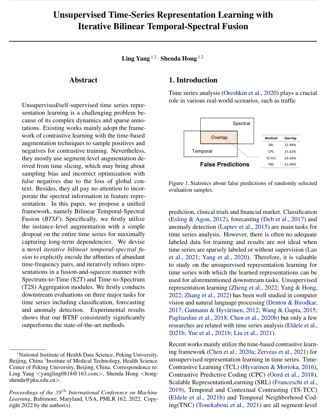
On the HAR test set, the paper compares errors made using temporal-only and spectral-only representations; for BTSF these are the features output by S2T and T2S, respectively. It counts errors common to both prediction sets and reports the common-error overlap as a percentage of each set. BTSF has 159 temporal-only errors, 163 spectral-only errors, and 152 shared errors, corresponding to overlaps of $96.60\%$ and $93.25\%$ . The comparison methods have substantially smaller overlaps: SRL, $32.53\%$ and $29.73\%$ ; CPC, $26.43\%$ and $23.66\%$ ; TS-TCC, $30.23\%$ and $27.94\%$ ; and TNC, $33.24\%$ and $30.59\%$ . This is evidence, in the paper's evaluation, that iterative fusion makes the two domain-specific representations much more concordant.

Additional representation diagnostics are qualitative: t-SNE plots show more distinct clusters for BTSF representations from the same HAR hidden state, while the alignment and uniformity plots are interpreted by the authors as showing well-aligned positive pairs and a more even feature distribution than TNC and the supervised model. The paper does not report numerical values for these plotted diagnostics.
Knowl 10 — Bilinear fusion couples gradient updates across domains
theoretical result
For BTSF's joint representation, the paper's gradient analysis finds that the update to temporal-encoder parameters depends on the spectral features, and the update to spectral-encoder parameters depends on the temporal features. The interaction-matrix gradient is linked to cross-domain products of temporal and spectral features. This establishes the authors' stated mechanism for cross-domain learning: temporal and spectral information directly influence each other's feature updates, rather than being combined only after independent feature extraction. The analysis omits the sigmoid derivative for simplicity and applies to the paper's bilinear joint-feature construction.

Coverage note — The additional forecasting visualizations, dataset descriptions, and individual per-dataset rows from the extended classification appendix are omitted because they corroborate the reported quantitative results without adding a distinct central method or finding.

References

1.Andrzejak, R. G., Lehnertz, K., Mormann, F., Rieke, C., David, P., and Elger, C. E. Indications of nonlinear deterministic and finite-dimensional structures in time series of brain electrical activity: Dependence on recording region and brain state. Physical Review E, 64(6):061907, 2001.
2.Anguita, D., Ghio, A., Oneto, L., Parra, X., Reyes-Ortiz, J. L., et al. A public domain dataset for human activity recognition using smartphones. In Esann, volume 3, pp. 3, 2013.
3.Audibert, J., Michiardi, P., Guyard, F., Marti, S., and Zuluaga, M. A. Usad: Unsupervised anomaly detection on multivariate time series. In Proceedings of the 26th ACM SIGKDD International Conference on Knowledge Discovery & Data Mining, pp. 3395–3404, 2020.
4.Bai, S., Kolter, J. Z., and Koltun, V. An empirical evaluation of generic convolutional and recurrent networks for sequence modeling. arXiv preprint arXiv:1803.01271, 2018.
5.Bayer, J., Soelch, M., Mirchev, A., Kayalibay, B., and van der Smagt, P. Mind the gap when conditioning amortised inference in sequential latent-variable models. arXiv preprint arXiv:2101.07046, 2021.
6.Braei, M. and Wagner, S. Anomaly detection in univariate time-series: A survey on the state-of-the-art. arXiv preprint arXiv:2004.00433, 2020.
7.Chen, T., Kornblith, S., Norouzi, M., and Hinton, G. A simple framework for contrastive learning of visual representations. In International conference on machine learning, pp. 1597–1607. PMLR, 2020a.
8.Chen, T., Kornblith, S., Norouzi, M., and Hinton, G. A simple framework for contrastive learning of visual representations. In Proceedings of the 37th International Conference on Machine Learning, volume 119 of Proceedings of Machine Learning Research, pp. 1597–1607, 13–18 Jul 2020b.
9.Chen, Y., Hu, B., Keogh, E., and Batista, G. E. Dtw-d: time series semi-supervised learning from a single example. In Proceedings of the 19th ACM SIGKDD international conference on Knowledge discovery and data mining, pp. 383–391, 2013.
10.Choi, E., Bahadori, M. T., Searles, E., Coffey, C., Thompson, M., Bost, J., Tejedor-Sojo, J., and Sun, J. Multi-layer representation learning for medical concepts. In Proceedings of the 22nd ACM SIGKDD International Conference on Knowledge Discovery and Data Mining, pp. 1495–1504, 2016.
11.Chung, J., Kastner, K., Dinh, L., Goel, K., Courville, A. C., and Bengio, Y. A recurrent latent variable model for sequential data. Advances in neural information processing systems, 28:2980–2988, 2015.
12.Deb, C., Zhang, F., Yang, J., Lee, S. E., and Shah, K. W. A review on time series forecasting techniques for building energy consumption. Renewable and Sustainable Energy Reviews, 74:902–924, 2017.
13.Dempster, A., Petitjean, F., and Webb, G. I. Rocket: exceptionally fast and accurate time series classification using random convolutional kernels. Data Mining and Knowledge Discovery, 34(5):1454–1495, 2020.
14.Denton, E. and Birodkar, V. Unsupervised learning of disentangled representations from video. arXiv preprint arXiv:1705.10915, 2017.
15.Eldele, E., Chen, Z., Liu, C., Wu, M., Kwoh, C.-K., Li, X., and Guan, C. An attention-based deep learning approach for sleep stage classification with single-channel eeg. IEEE Transactions on Neural Systems and Rehabilitation Engineering, 29:809–818, 2021a.
16.Eldele, E., Ragab, M., Chen, Z., Wu, M., Kwoh, C. K., Li, X., and Guan, C. Time-series representation learning via temporal and contextual contrasting. arXiv preprint arXiv:2106.14112, 2021b.
17.Esling, P. and Agon, C. Time-series data mining. ACM Computing Surveys (CSUR), 45(1):1–34, 2012.
18.Forestier, G., Petitjean, F., Dau, H. A., Webb, G. I., and Keogh, E. Generating synthetic time series to augment sparse datasets. In 2017 IEEE international conference on data mining (ICDM), pp. 865–870. IEEE, 2017.
19.Fraccaro, M., Sønderby, S. K., Paquet, U., and Winther, O. Sequential neural models with stochastic layers. arXiv preprint arXiv:1605.07571, 2016.
20.Franceschi, J.-Y., Dieuleveut, A., and Jaggi, M. Unsupervised scalable representation learning for multivariate time series. Advances In Neural Information Processing Systems 32 (Nips 2019), 32(CONF), 2019.
21.Goh, J., Adepu, S., Junejo, K. N., and Mathur, A. A dataset to support research in the design of secure water treatment systems. In International conference on critical information infrastructures security, pp. 88–99. Springer, 2016.
22.Goldberger, A. L., Amaral, L. A., Glass, L., Hausdorff, J. M., Ivanov, P. C., Mark, R. G., Mietus, J. E., Moody, G. B., Peng, C.-K., and Stanley, H. E. Physiobank, physiotoolkit, and physionet: components of a new research resource for complex physiologic signals. circulation, 101(23):e215–e220, 2000.
23.Gutmann, M. and Hyvarinen, A. Noise-contrastive estimation: A new estimation principle for unnormalized statistical models. In Teh, Y. W. and Titterington, M. (eds.), Proceedings of the Thirteenth International Conference on Artificial Intelligence and Statistics, volume 9 of Proceedings of Machine Learning Research, pp. 297–304, Chia Laguna Resort, Sardinia, Italy, 13–15 May 2010.
24.Gutmann, M. U. and Hyvarinen, A. Noise-contrastive estimation of unnormalized statistical models, with applications to natural image statistics. Journal of Machine Learning Research, 13(2), 2012.
25.Hundman, K., Constantinou, V., Laporte, C., Colwell, I., and Soderstrom, T. Detecting spacecraft anomalies using lstms and nonparametric dynamic thresholding. In Proceedings of the 24th ACM SIGKDD international conference on knowledge discovery & data mining, pp. 387–395, 2018.
26.Hyvarinen, A. and Morioka, H. Unsupervised feature extraction by time-contrastive learning and nonlinear ica. arXiv preprint arXiv:1605.06336, 2016.
27.Iwana, B. K. and Uchida, S. An empirical survey of data augmentation for time series classification with neural networks. Plos one, 16(7):e0254841, 2021a.
28.Iwana, B. K. and Uchida, S. Time series data augmentation for neural networks by time warping with a discriminative teacher. In 2020 25th International Conference on Pattern Recognition (ICPR), pp. 3558–3565. IEEE, 2021b.
29.Kamycki, K., Kapuscinski, T., and Oszust, M. Data augmentation with suboptimal warping for time-series classification. Sensors, 20(1):98, 2020.
30.Kingma, D. P. and Ba, J. Adam: A method for stochastic optimization, 2017.
31.Krishna, K. and Murty, M. N. Genetic k-means algorithm. IEEE Transactions on Systems, Man, and Cybernetics, Part B (Cybernetics), 29(3):433–439, 1999.
32.Krishnan, R., Shalit, U., and Sontag, D. Structured inference networks for nonlinear state space models. In Proceedings of the AAAI Conference on Artificial Intelligence, volume 31, 2017.
33.Lan, X., Ng, D., Hong, S., and Feng, M. Intra-inter subject self-supervised learning for multivariate cardiac signals, 2021.
34.Langkvist, M., Karlsson, L., and Loutfi, A. A review of unsupervised feature learning and deep learning for time-series modeling. Pattern Recognition Letters, 42:11–24, 2014.
35.Laptev, N., Amizadeh, S., and Flint, I. Generic and scalable framework for automated time-series anomaly detection. In Proceedings of the 21th ACM SIGKDD International Conference on Knowledge Discovery and Data Mining, pp. 1939–1947, New York, NY, USA, 2015.
36.Lei, Q., Yi, J., Vaculin, R., Wu, L., and Dhillon, I. S. Similarity preserving representation learning for time series clustering. arXiv preprint arXiv:1702.03584, 2017.
37.Liu, X., Liang, Y., Zheng, Y., Hooi, B., and Zimmermann, R. Spatio-temporal graph contrastive learning. arXiv preprint arXiv:2108.11873, 2021.
38.Lyu, X., Hueser, M., Hyland, S. L., Zerveas, G., and Raetsch, G. Improving clinical predictions through unsupervised time series representation learning. arXiv preprint arXiv:1812.00490, 2018.
39.Ma, Q., Zheng, J., Li, S., and Cottrell, G. W. Learning representations for time series clustering. Advances in neural information processing systems, 32:3781–3791, 2019.
40.Malhotra, P., TV, V., Vig, L., Agarwal, P., and Shroff, G. Timenet: Pre-trained deep recurrent neural network for time series classification. arXiv preprint arXiv:1706.08838, 2017.
41.Mathur, A. P. and Tippenhauer, N. O. Swat: A water treatment testbed for research and training on ics security. In 2016 international workshop on cyber-physical systems for smart water networks (CySWater), pp. 31–36. IEEE, 2016.
42.Mikolov, T., Chen, K., Corrado, G., and Dean, J. Efficient estimation of word representations in vector space. arXiv preprint arXiv:1301.3781, 2013.
43.Moody, G. A new method for detecting atrial fibrillation using rr intervals. Computers in Cardiology, pp. 227–230, 1983.
44.Oord, A. v. d., Li, Y., and Vinyals, O. Representation learning with contrastive predictive coding. arXiv preprint arXiv:1807.03748, 2018.
45.Oreshkin, B. N., Carpov, D., Chapados, N., and Bengio, Y. N-beats: Neural basis expansion analysis for interpretable time series forecasting. In International Conference on Learning Representations, 2020.
46.Pagliardini, M., Gupta, P., and Jaggi, M. Unsupervised learning of sentence embeddings using compositional n-gram features. In Proceedings of the 2018 Conference of the North American Chapter of the Association for Computational Linguistics: Human Language Technologies, Volume 1 (Long Papers), pp. 528–540, 2018.
47.Paszke, A., Gross, S., Chintala, S., Chanan, G., Yang, E., DeVito, Z., Lin, Z., Desmaison, A., Antiga, L., and Lerer, A. Automatic differentiation in pytorch. 2017.
48.Srivastava, N., Hinton, G., Krizhevsky, A., Sutskever, I., and Salakhutdinov, R. Dropout: A simple way to prevent neural networks from overfitting. Journal of Machine Learning Research, 15(56):1929–1958, 2014.
49.Su, Y., Zhao, Y., Niu, C., Liu, R., Sun, W., and Pei, D. Robust anomaly detection for multivariate time series through stochastic recurrent neural network. In Proceedings of the 25th ACM SIGKDD International Conference on Knowledge Discovery & Data Mining, pp. 2828–2837, 2019.
50.Tonekaboni, S., Eytan, D., and Goldenberg, A. Unsupervised representation learning for time series with temporal neighborhood coding. arXiv preprint arXiv:2106.00750, 2021.
51.Van der Maaten, L. and Hinton, G. Visualizing data using t-sne. Journal of machine learning research, 9(11), 2008.
52.Wang, T. and Isola, P. Understanding contrastive representation learning through alignment and uniformity on the hypersphere. In International Conference on Machine Learning, pp. 9929–9939. PMLR, 2020.
53.Wang, X. and Gupta, A. Unsupervised learning of visual representations using videos. In Proceedings of the IEEE international conference on computer vision, pp. 2794–2802, 2015.
54.Yang, L. and Hong, S. Omni-granular ego-semantic propagation for self-supervised graph representation learning. arXiv preprint arXiv:2205.15746, 2022.
55.Yang, L., Li, L., Zhang, Z., Zhou, X., Zhou, E., and Liu, Y. Dpgn: Distribution propagation graph network for few-shot learning. In Proceedings of the IEEE/CVF Conference on Computer Vision and Pattern Recognition, pp. 13390–13399, 2020.
56.Yue, Z., Wang, Y., Duan, J., Yang, T., Huang, C., Tong, Y., and Xu, B. Ts2vec: Towards universal representation of time series. arXiv preprint arXiv:2106.10466, 2021a.
57.Yue, Z., Wang, Y., Duan, J., Yang, T., Huang, C., and Xu, B. Learning timestamp-level representations for time series with hierarchical contrastive loss. arXiv preprint arXiv:2106.10466, 2021b.
58.Zerveas, G., Jayaraman, S., Patel, D., Bhamidipaty, A., and Eickhoff, C. A transformer-based framework for multivariate time series representation learning. In Proceedings of the 27th ACM SIGKDD Conference on Knowledge Discovery & Data Mining, pp. 2114–2124, 2021.
59.Zhang, W., Yang, L., Geng, S., and Hong, S. Cross reconstruction transformer for self-supervised time series representation learning. arXiv preprint arXiv:2205.09928, 2022.
60.Zheng, J., Yang, L., Wang, H., Yang, C., Li, Y., Hu, X., and Hong, S. Spatial autoregressive coding for graph neural recommendation. arXiv preprint arXiv:2205.09489, 2022.
61.Zhou, H., Zhang, S., Peng, J., Zhang, S., Li, J., Xiong, H., and Zhang, W. Informer: Beyond efficient transformer for long sequence time-series forecasting, 2021.

Citation

MLA

Yang, L., and S. Hong. “Unsupervised Time-Series Representation Learning with Iterative Bilinear Temporal-Spectral Fusion”. International Conference on Machine Learning, vol. 162, 2022, pp. 25038–54, https://proceedings.mlr.press/v162/yang22e.html.

APA

Yang, L., & Hong, S. (2022). Unsupervised Time-Series Representation Learning with Iterative Bilinear Temporal-Spectral Fusion. International Conference on Machine Learning, 162, 25038–25054. https://proceedings.mlr.press/v162/yang22e.html

Chicago

Yang, L., and S. Hong. 2022. “Unsupervised Time-Series Representation Learning with Iterative Bilinear Temporal-Spectral Fusion”. International Conference on Machine Learning 162: 25038–54. https://proceedings.mlr.press/v162/yang22e.html.

Harvard

Yang, L. and Hong, S. (2022) “Unsupervised Time-Series Representation Learning with Iterative Bilinear Temporal-Spectral Fusion”, International Conference on Machine Learning. PMLR, pp. 25038–25054. Available at: https://proceedings.mlr.press/v162/yang22e.html.

Vancouver

1. Yang L, Hong S (2022) Unsupervised Time-Series Representation Learning with Iterative Bilinear Temporal-Spectral Fusion. In: International Conference on Machine Learning. PMLR, pp 25038–25054

BibTeX

@InProceedings{pmlr-v162-yang22e,
  title = 	 {Unsupervised Time-Series Representation Learning with Iterative Bilinear Temporal-Spectral Fusion},
  author =       {Yang, Ling and Hong, Shenda},
  booktitle = 	 {Proceedings of the 39th International Conference on Machine Learning},
  pages = 	 {25038--25054},
  year = 	 {2022},
  editor = 	 {Chaudhuri, Kamalika and Jegelka, Stefanie and Song, Le and Szepesvari, Csaba and Niu, Gang and Sabato, Sivan},
  volume = 	 {162},
  series = 	 {Proceedings of Machine Learning Research},
  month = 	 {17--23 Jul},
  publisher =    {PMLR},
  pdf = 	 {https://proceedings.mlr.press/v162/yang22e/yang22e.pdf},
  url = 	 {https://proceedings.mlr.press/v162/yang22e.html},
  abstract = 	 {Unsupervised/self-supervised time series representation learning is a challenging problem because of its complex dynamics and sparse annotations. Existing works mainly adopt the framework of contrastive learning with the time-based augmentation techniques to sample positives and negatives for contrastive training. Nevertheless, they mostly use segment-level augmentation derived from time slicing, which may bring about sampling bias and incorrect optimization with false negatives due to the loss of global context. Besides, they all pay no attention to incorporate the spectral information in feature representation. In this paper, we propose a unified framework, namely Bilinear Temporal-Spectral Fusion (BTSF). Specifically, we firstly utilize the instance-level augmentation with a simple dropout on the entire time series for maximally capturing long-term dependencies. We devise a novel iterative bilinear temporal-spectral fusion to explicitly encode the affinities of abundant time-frequency pairs, and iteratively refines representations in a fusion-and-squeeze manner with Spectrum-to-Time (S2T) and Time-to-Spectrum (T2S) Aggregation modules. We firstly conducts downstream evaluations on three major tasks for time series including classification, forecasting and anomaly detection. Experimental results shows that our BTSF consistently significantly outperforms the state-of-the-art methods.}
}

Metadata:DOI registry

Access the Paper

This paper is available from its original source. Click below to access the PDF.

Open PDF

License: https://creativecommons.org/licenses/by/4.0/

Unsupervised Time-Series Representation Learning with Iterative Bilinear Temporal-Spectral Fusion

Abstract

Topics

Keywords

Table of Contents

Knowls

Knowl 1 — BTSF iteratively fuses temporal and spectral representations

Knowl 2 — Whole-series dropout constructs instance-level contrastive views

Knowl 3 — Low-rank bilinear fusion produces the joint representation

Knowl 4 — Contrastive training attracts dropout views and separates other variables

Knowl 5 — BTSF improves classification across the reported benchmarks

Knowl 6 — BTSF has the lowest reported forecasting errors across four datasets

Knowl 7 — BTSF leads the reported anomaly-detection comparisons

Knowl 8 — Ablations identify dropout and iterative bilinear fusion as key components

Knowl 9 — Temporal and spectral predictions become strongly aligned under BTSF

Knowl 10 — Bilinear fusion couples gradient updates across domains

References

Citation

BibTeX

Access the Paper