Class-Balanced Loss Based on Effective Number of Samples

Yin CuiMenglin JiaTsung-Yi LinYang SongSerge J. Belongie

article2019CVPR3,353 citations

Develops a theoretically grounded loss re-weighting method based on the effective number of samples that captures diminishing data returns to significantly improve classification accuracy on long-tailed visual recognition benchmarks.

Listen

Real-world visual recognition datasets often follow long-tailed distributions, in which a small number of classes account for most examples while the majority of classes are represented by far fewer samples. Convolutional neural networks trained on such data typically perform poorly on the under-represented classes, limiting their usefulness for applications that rely on fine-grained or diverse categories.

The work develops a class-balanced loss that re-weights training examples according to an effective number of samples per class rather than raw class frequency. The authors first introduce a theoretical model that treats data sampling as a simplified random-covering process: each sample occupies a small neighboring region in feature space, and successive samples may overlap completely with previously seen data. This leads to a closed-form expression for the effective number of samples, (1β^n)/(1β), where n is the observed count for a class and β is a single hyper-parameter that controls the rate at which additional samples cease to add new information. The resulting weighting factor is then inserted into standard loss functionssoftmax cross-entropy, sigmoid cross-entropy, and focal lossproducing a model- and loss-agnostic class-balanced term.

Extensive experiments were performed on artificially long-tailed versions of CIFAR-10 and CIFAR-100 (imbalance factors 10200), the large-scale iNaturalist 2017 and 2018 datasets (more than 5 000 and 8 000 classes, respectively), and the relatively balanced ILSVRC 2012 benchmark. Networks were trained from scratch with ResNet architectures of varying depth, and performance was measured by top-1 and top-5 classification error.

Across these benchmarks the class-balanced losses consistently outperform their unweighted counterparts. On long-tailed CIFAR the best configurations reduce error by 38 percentage points relative to plain softmax or focal loss; on iNaturalist the gains exceed 34 points for ResNet-50 and allow a 50-layer network trained with the new loss to match or surpass a 152-layer network trained with softmax. Even on ILSVRC 2012 the method yields modest but reliable improvements. The magnitude of improvement grows with the degree of imbalance, and the optimal β is larger for coarse-grained datasets than for fine-grained ones, confirming that the framework automatically adapts the strength of re-weighting to the underlying data redundancy.

These results indicate that a theoretically grounded adjustment of per-class loss weights can substantially mitigate the bias toward dominant classes without the overfitting or information loss associated with resampling. The approach therefore offers a practical route to higher accuracy on the skewed distributions typical of real-world imagery, at negligible extra computational cost.

The principal remaining uncertainties are the need to select β via cross-validation and the assumption that a single dataset-level N suffices for all classes. Future work could incorporate class-specific estimates of unique prototypes or learned adaptive weighting to reduce this tuning burden. In the meantime, practitioners facing long-tailed recognition tasks can obtain immediate gains by replacing a standard loss with its class-balanced counterpart and validating β on a modest held-out set.

No sufficiently relevant recommendations were found.

  • Paper: Supervised Contrastive Learning, Prannay Khosla et al. (2020). This work extends the exploration of loss design for classification by introducing a supervised contrastive loss that structures representation geometry directly from class labels.
Cover for Class-Balanced Loss Based on Effective Number of Samples

Abstract

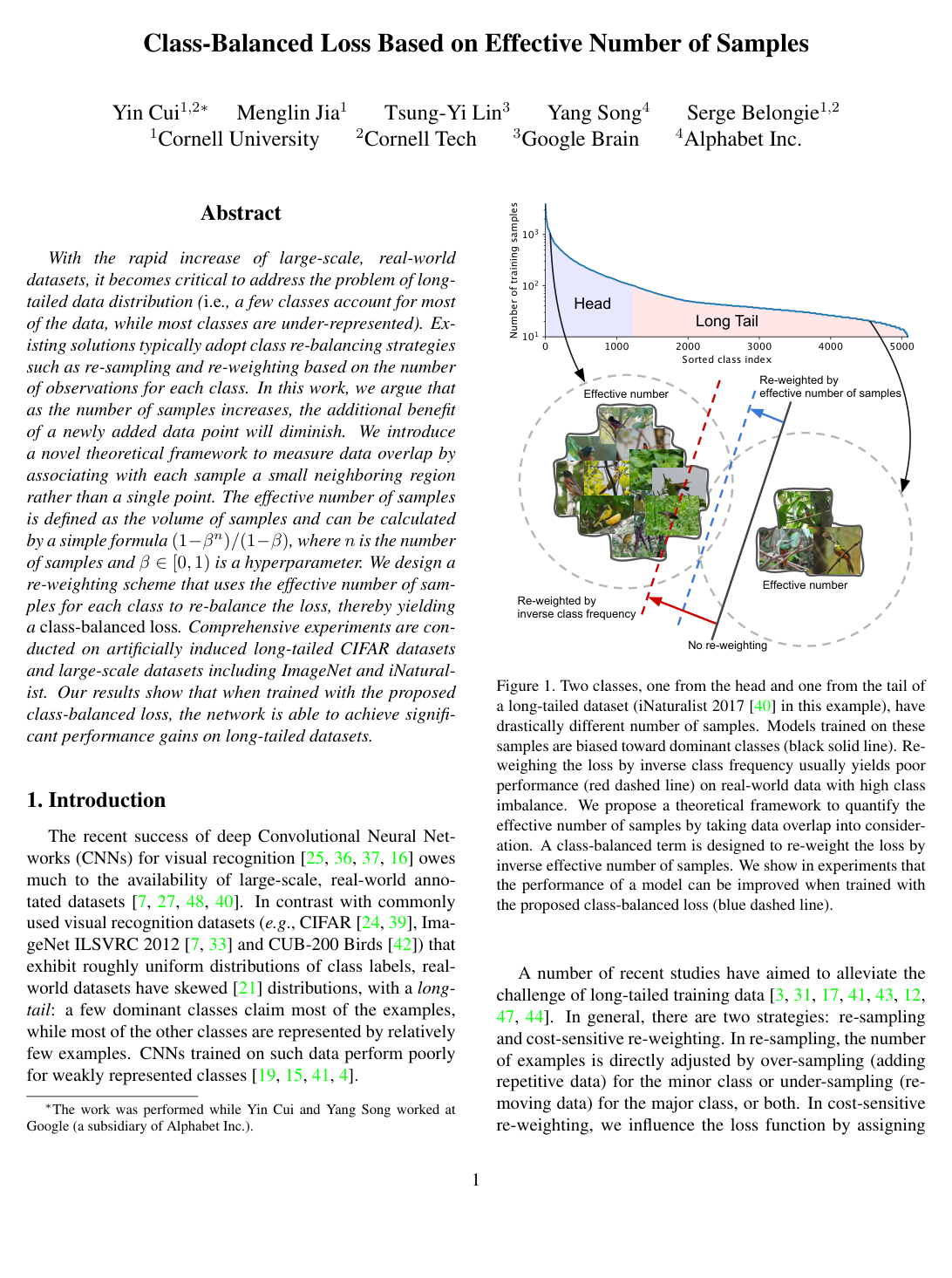
With the rapid increase of large-scale, real-world datasets, it becomes critical to address the problem of long-tailed data distribution (i.e., a few classes account for most of the data, while most classes are under-represented). Existing solutions typically adopt class re-balancing strategies such as re-sampling and re-weighting based on the number of observations for each class. In this work, we argue that as the number of samples increases, the additional benefit of a newly added data point will diminish. We introduce a novel theoretical framework to measure data overlap by associating with each sample a small neighboring region rather than a single point. The effective number of samples is defined as the volume of samples and can be calculated by a simple formula (1βn)/(1β)(1-\beta^{n})/(1-\beta), where nn is the number of samples and β[0,1)\beta \in [0,1) is a hyperparameter. We design a re-weighting scheme that uses the effective number of samples for each class to re-balance the loss, thereby yielding a class-balanced loss. Comprehensive experiments are conducted on artificially induced long-tailed CIFAR datasets and large-scale datasets including ImageNet and iNaturalist. Our results show that when trained with the proposed class-balanced loss, the network is able to achieve significant performance gains on long-tailed datasets.

Table of Contents

  • 1. Introduction
  • 2. Related Work
  • 3. Effective Number of Samples
  • 3.1. Data Sampling as Random Covering
  • 3.2. Mathematical Formulation
  • 4. Class-Balanced Loss
  • 4.1. Class-Balanced Softmax Cross-Entropy Loss
  • 4.2. Class-Balanced Sigmoid Cross-Entropy Loss
  • 4.3. Class-Balanced Focal Loss
  • 5. Experiments
  • 5.1. Datasets
  • 5.2. Implementation
  • 5.3. Visual Recognition on Long-Tailed CIFAR
  • 5.4. Visual Recognition on Large-Scale Datasets
  • 6. Conclusion and Discussion

Knowls

  1. Knowl 1 — Effective Number of Samples Formulation

    theoretical result

    Under a simplified random covering framework, the feature space of a given class is modeled as a set SS with total volume N1N \ge 1. Each sampled data point is treated as a subset of unit volume 11 that is either entirely within the region covered by previously sampled data (with probability p=En1/Np = E_{n-1}/N) or entirely outside (with probability 1p1-p). The effective number of samples EnE_n, defined as the expected volume covered after drawing nn samples (nZ>0n \in \mathbb{Z}_{>0}), is given by:

    En=1βn1βE_n = \frac{1 - \beta^n}{1 - \beta}

    where β=N1N[0,1)\beta = \frac{N - 1}{N} \in [0, 1) parameterizes the effective prototype volume N=1/(1β)N = 1 / (1 - \beta). Equivalently, the effective number can be expanded as the sum of geometrically diminishing marginal contributions:

    En=j=1nβj1E_n = \sum_{j=1}^n \beta^{j-1}

    where the jj-th sampled data point adds a marginal volume contribution of βj1\beta^{j-1} to the coverage.

  2. Knowl 2 — Class-Balanced Loss Weighting Framework

    model/method

    To mitigate the bias caused by class imbalance during deep convolutional neural network training without assuming sample difficulty or explicit data distributions, the class-balanced (CB) loss weights the loss of each sample inversely proportional to the effective number of samples in its ground-truth class.

    For an input sample xx with ground-truth class label y{1,2,,C}y \in \{1, 2, \dots, C\} belonging to a dataset of CC classes where class ii contains nin_i training examples, the class-balanced loss is defined as:

    CB(p,y)=1EnyL(p,y)=1β1βnyL(p,y)\text{CB}(p, y) = \frac{1}{E_{n_y}} \mathcal{L}(p, y) = \frac{1 - \beta}{1 - \beta^{n_y}} \mathcal{L}(p, y)

    where p[0,1]Cp \in [0, 1]^C is the vector of model-predicted class probabilities, L(p,y)\mathcal{L}(p, y) is a base loss function, and β[0,1)\beta \in [0, 1) is a dataset-level hyperparameter. To keep the total loss scale invariant across datasets, the weighting factors αi1/Eni\alpha_i \propto 1/E_{n_i} can be normalized such that i=1Cαi=C\sum_{i=1}^C \alpha_i = C.

    The hyperparameter β\beta smoothly adjusts the re-weighting term between uniform unweighted training (β=0\beta = 0, where Eny=1E_{n_y} = 1) and inverse class-frequency re-weighting (β1\beta \to 1, where EnynyE_{n_y} \to n_y).

  3. Knowl 3 — Class-Balanced Formulations of Softmax, Sigmoid, and Focal Losses

    model/method

    The class-balanced weighting factor 1β1βny\frac{1 - \beta}{1 - \beta^{n_y}} can be applied to standard loss functions for multi-class visual recognition, where z=[z1,z2,,zC]z = [z_1, z_2, \dots, z_C]^\top is the vector of model output logits across CC classes, y{1,,C}y \in \{1, \dots, C\} is the ground-truth class index, nyn_y is the number of training examples in class yy, and β[0,1)\beta \in [0, 1):

    1. Class-Balanced Softmax Cross-Entropy Loss:

    CBsoftmax(z,y)=1β1βnylog(exp(zy)j=1Cexp(zj))\text{CB}_{\text{softmax}}(z, y) = - \frac{1 - \beta}{1 - \beta^{n_y}} \log\left( \frac{\exp(z_y)}{\sum_{j=1}^C \exp(z_j)} \right)

    1. Class-Balanced Sigmoid Cross-Entropy Loss: Defining zit=ziz_i^t = z_i if i=yi = y and zit=ziz_i^t = -z_i otherwise:

    CBsigmoid(z,y)=1β1βnyi=1Clog(11+exp(zit))\text{CB}_{\text{sigmoid}}(z, y) = - \frac{1 - \beta}{1 - \beta^{n_y}} \sum_{i=1}^C \log\left( \frac{1}{1 + \exp(-z_i^t)} \right)

    1. Class-Balanced Focal Loss: Modulating the loss for well-classified samples via focusing parameter γ0\gamma \ge 0, where pit=sigmoid(zit)=11+exp(zit)p_i^t = \text{sigmoid}(z_i^t) = \frac{1}{1 + \exp(-z_i^t)}:

    CBfocal(z,y)=1β1βnyi=1C(1pit)γlog(pit)\text{CB}_{\text{focal}}(z, y) = - \frac{1 - \beta}{1 - \beta^{n_y}} \sum_{i=1}^C (1 - p_i^t)^\gamma \log(p_i^t)

    In this formulation, the class-balanced factor 1β1βny\frac{1 - \beta}{1 - \beta^{n_y}} provides an explicit, sample-size-grounded method to set the αt\alpha_t parameter of α\alpha-balanced focal loss based on the effective number of samples.

  4. Knowl 4 — Asymptotic Properties and Prototype Capacity of the Effective Number Parameter

    theoretical result

    The effective number of samples En=1βn1βE_n = \frac{1 - \beta^n}{1 - \beta} exhibits the following asymptotic properties with respect to the hyperparameter β[0,1)\beta \in [0, 1) and the total prototype capacity N=11βN = \frac{1}{1 - \beta}:

    1. Single Prototype Limit (β=0\beta = 0, N=1N = 1):

    limβ0En=1\lim_{\beta \to 0} E_n = 1

    This assumes all data points in a class represent a single underlying prototype (e.g., generated entirely through heavy data augmentations or transformations), resulting in equal weighting for all classes regardless of sample count nn.

    1. Infinite Prototype Limit (β1\beta \to 1, NN \to \infty):

    limβ1En=limβ11βn1β=n\lim_{\beta \to 1} E_n = \lim_{\beta \to 1} \frac{1 - \beta^n}{1 - \beta} = n

    This assumes every data point in a class is distinct and non-overlapping, reducing class-balanced weighting directly to inverse class-frequency weighting 1n\frac{1}{n}.

    The quantity N=limnEn=11βN = \lim_{n \to \infty} E_n = \frac{1}{1 - \beta} represents the maximum number of unique prototypes contained in a class. Stronger data augmentations reduce the effective number of unique prototypes, corresponding to smaller values of NN and smaller optimal values of β\beta.

  5. Knowl 5 — Bias Initialization and Training Stabilization for Sigmoid-Based Multi-Class Loss

    model/method

    When using sigmoid cross-entropy or focal loss for multi-class recognition, initializing the final linear classification layer with bias b=0b = 0 results in initial predicted class probabilities of approximately 0.50.5, which produces large initial loss values that destabilize network optimization.

    To stabilize training under sigmoid-based multi-class losses:

    1. Assume a uniform class prior π=1/C\pi = 1 / C, where CC is the total number of classes.
    2. Initialize the bias parameter bb of the final linear layer as:

    b=log(1ππ)=log(C1)b = - \log\left( \frac{1 - \pi}{\pi} \right) = - \log(C - 1)

    1. Remove L2L_2 regularization (weight decay) from the bias parameter bb of the final classification layer.

    Furthermore, when training deep residual networks on highly imbalanced data, decaying the learning rate by a factor of 0.010.01 (rather than 0.10.1) at learning rate drop steps prevents training instability where training loss and validation error drift upward after the drop.

  6. Knowl 6 — Benchmark Results of ResNet-32 on Long-Tailed CIFAR Datasets

    data/table

    On artificially induced long-tailed versions of CIFAR-10 and CIFAR-100 with exponential sample drop (n=niμin = n_i \mu^i, where imbalance factor is the ratio of maximum to minimum class sample count), ResNet-32 models trained with class-balanced (CB) losses outperform unweighted softmax cross-entropy, sigmoid cross-entropy, and focal loss across all imbalance factors.

    Dataset Long-Tailed CIFAR-10 Long-Tailed CIFAR-100
    Imbalance Factor 200 100 50 20 10 1 200 100 50 20 10 1
    Softmax 34.32 29.64 25.19 17.77 13.61 6.61 65.16 61.68 56.15 48.86 44.29 29.07
    Sigmoid 34.51 29.55 23.84 16.40 12.97 6.36 64.39 61.22 55.85 48.57 44.73 28.39
    Focal (γ=0.5\gamma = 0.5) 36.00 29.77 23.28 17.11 13.19 6.75 65.00 61.31 55.88 48.90 44.30 28.55
    Focal (γ=1.0\gamma = 1.0) 34.71 29.62 23.29 17.24 13.34 6.60 64.38 61.59 55.68 48.05 44.22 28.85
    Focal (γ=2.0\gamma = 2.0) 35.12 30.41 23.48 16.77 13.68 6.61 65.25 61.61 56.30 48.98 45.00 28.52
    Class-Balanced 31.11 25.43 20.73 15.64 12.51 6.36 63.77 60.40 54.68 47.41 42.01 28.39
    Loss Type SM Focal Focal SM SGM SGM Focal Focal SGM Focal Focal SGM
    β\beta 0.9999 0.9999 0.9999 0.9999 0.9999 - 0.9 0.9 0.99 0.99 0.999 -
    γ\gamma - 1.0 2.0 - - - 1.0 1.0 - 0.5 0.5 -

    The table lists test set classification error rates (%). The best class-balanced loss configurations achieve error reductions over the best unweighted baselines of up to 4.21%4.21\% on CIFAR-10 (imbalance factor 100) and 2.28%2.28\% on CIFAR-100 (imbalance factor 10). When classes are balanced (imbalance factor 1), the class-balanced weight is 1 and the loss reduces to the original base loss.

  7. Knowl 7 — Performance of Class-Balanced Focal Loss on Large-Scale Datasets

    data/table

    On real-world long-tailed datasets (iNaturalist 2017 with 5,089 classes; iNaturalist 2018 with 8,142 classes) and standard large-scale benchmarks (ILSVRC 2012 ImageNet with 1,000 classes), training ResNets from scratch with class-balanced focal loss (β=0.999\beta = 0.999, γ=0.5\gamma = 0.5) outperforms standard softmax cross-entropy loss across network depths and input resolutions.

    iNaturalist 2017 iNaturalist 2018 ILSVRC 2012
    Network Loss β\beta γ\gamma Top-1 Top-5 Top-1 Top-5 Top-1 Top-5
    ResNet-50 Softmax - - 45.38 22.67 42.86 21.31 23.92 7.03
    ResNet-101 Softmax - - 42.57 20.42 39.47 18.86 22.65 6.47
    ResNet-152 Softmax - - 41.42 19.47 38.61 18.07 21.68 5.92
    ResNet-50 CB Focal 0.999 0.5 41.92 20.92 38.88 18.97 22.71 6.72
    ResNet-101 CB Focal 0.999 0.5 39.06 18.96 36.12 17.18 21.57 5.91
    ResNet-152 CB Focal 0.999 0.5 38.06 18.42 35.21 16.34 20.87 5.61
    ResNet-50 (320×320320\times320) CB Focal 0.999 0.5 38.16 18.28 35.84 16.85 21.99 6.27
    ResNet-101 (320×320320\times320) CB Focal 0.999 0.5 34.96 15.90 32.02 14.27 20.25 5.34
    ResNet-152 (320×320320\times320) CB Focal 0.999 0.5 33.73 14.96 30.95 13.54 19.72 4.97

    The table presents validation error rates (%). On iNaturalist 2017 and 2018, class-balanced focal loss lowers Top-1 error by 3.46%3.46\% and 3.98%3.98\% on ResNet-50, allowing a ResNet-50 model to match or exceed the accuracy of a ResNet-152 trained with softmax cross-entropy. On ILSVRC 2012, class-balanced focal loss reduces ResNet-50 Top-1 error by 1.21%1.21\% compared to softmax cross-entropy.

  8. Knowl 8 — Effect of Class Granularity on Optimal Hyperparameter Beta

    empirical result

    The optimal value of the hyperparameter β\beta in class-balanced loss is governed by class granularity:

    • On coarse-grained datasets such as CIFAR-10 (10 distinct visual classes), classification performance improves monotonically as β1\beta \to 1, with β=0.9999\beta = 0.9999 uniformly yielding the lowest error rates across all imbalance factors. Coarse classes have a large prototype capacity NN, meaning samples share less overlap and effective sample size scales close to linear sample count nn.
    • On fine-grained datasets such as CIFAR-100 (100 sub-classes) and CIFAR-20 (20 coarse classes), large values like β=0.9999\beta = 0.9999 degrade accuracy, while smaller values (β{0.9,0.99,0.999}\beta \in \{0.9, 0.99, 0.999\}) yield the best performance. Fine-grained categories have smaller intrinsic prototype spaces N=1/(1β)N = 1/(1-\beta) due to high visual similarity, causing the effective number of samples to saturate rapidly. As a result, direct inverse frequency weighting (β1\beta \to 1) over-penalizes frequent classes, whereas smaller β\beta values provide smoother and more accurate re-balancing weights.

Coverage note — None was omitted; all core theoretical formulations, class-balanced loss variants, training stabilization techniques, and empirical results across CIFAR, ImageNet, and iNaturalist datasets are covered.

References

  1. 1.The iNaturalist 2018 Competition Dataset. https://github.com/visipedia/inat_comp.
  2. 2.M. Abadi, P. Barham, J. Chen, Z. Chen, A. Davis, J. Dean, M. Devin, S. Ghemawat, G. Irving, M. Isard, et al. Tensorflow: A system for large-scale machine learning. In OSDI, 2016.
  3. 3.S. Bengio. Sharing representations for long tail computer vision problems. In ICMI, 2015.
  4. 4.M. Buda, A. Maki, and M. A. Mazurowski. A systematic study of the class imbalance problem in convolutional neural networks. Neural Networks, 2018.
  5. 5.N. V. Chawla, K. W. Bowyer, L. O. Hall, and W. P. Kegelmeyer. Smote: synthetic minority over-sampling technique. JAIR, 2002.
  6. 6.Y. Cui, Y. Song, C. Sun, A. Howard, and S. Belongie. Large scale fine-grained categorization and domain-specific transfer learning. In CVPR, 2018.
  7. 7.J. Deng, W. Dong, R. Socher, L.-J. Li, K. Li, and L. Fei-Fei. Imagenet: A large-scale hierarchical image database. In CVPR, 2009.
  8. 8.Q. Dong, S. Gong, and X. Zhu. Class rectification hard mining for imbalanced deep learning. In ICCV, 2017.
  9. 9.C. Drummond, R. C. Holte, et al. C4. 5, class imbalance, and cost sensitivity: why under-sampling beats over-sampling. In ICML Workshop, 2003.
  10. 10.C. Elkan. The foundations of cost-sensitive learning. In IJCAI, 2001.
  11. 11.Y. Freund and R. E. Schapire. A decision-theoretic generalization of on-line learning and an application to boosting. Journal of computer and system sciences, 1997.
  12. 12.Y. Geifman and R. El-Yaniv. Deep active learning over the long tail. arXiv preprint arXiv:1711.00941, 2017.
  13. 13.P. Goyal, P. Dollár, R. Girshick, P. Noordhuis, L. Wesolowski, A. Kyrola, A. Tulloch, Y. Jia, and K. He. Accurate, large minibatch sgd: training imagenet in 1 hour. arXiv preprint arXiv:1706.02677, 2017.
  14. 14.H. He, Y. Bai, E. A. Garcia, and S. Li. Adasyn: Adaptive synthetic sampling approach for imbalanced learning. In IEEE International Joint Conference on Neural Networks, 2008.
  15. 15.H. He and E. A. Garcia. Learning from imbalanced data. IEEE Transactions on Knowledge & Data Engineering, 2008.
  16. 16.K. He, X. Zhang, S. Ren, and J. Sun. Deep residual learning for image recognition. In CVPR, 2016.
  17. 17.C. Huang, Y. Li, C. Change Loy, and X. Tang. Learning deep representation for imbalanced classification. In CVPR, 2016.
  18. 18.S. Janson. Random coverings in several dimensions. Acta Mathematica, 1986.
  19. 19.N. Japkowicz and S. Stephen. The class imbalance problem: A systematic study. Intelligent data analysis, 2002.
  20. 20.H. Kahn and A. W. Marshall. Methods of reducing sample size in monte carlo computations. Journal of the Operations Research Society of America, 1953.
  21. 21.M. G. Kendall et al. The advanced theory of statistics. The advanced theory of statistics., (2nd Ed), 1946.
  22. 22.S. H. Khan, M. Hayat, M. Bennamoun, F. A. Sohel, and R. Togneri. Cost-sensitive learning of deep feature representations from imbalanced data. IEEE transactions on neural networks and learning systems, 2018.
  23. 23.P. W. Koh and P. Liang. Understanding black-box predictions via influence functions. In ICML, 2017.
  24. 24.A. Krizhevsky and G. Hinton. Learning multiple layers of features from tiny images. Technical report, Citeseer, 2009.
  25. 25.A. Krizhevsky, I. Sutskever, and G. E. Hinton. Imagenet classification with deep convolutional neural networks. In Neural Information Processing Systems, 2012.
  26. 26.T.-Y. Lin, P. Goyal, R. Girshick, K. He, and P. Dollár. Focal loss for dense object detection. PAMI, 2018.
  27. 27.T.-Y. Lin, M. Maire, S. Belongie, J. Hays, P. Perona, D. Ramanan, P. Dollár, and C. L. Zitnick. Microsoft coco: Common objects in context. In ECCV, 2014.
  28. 28.D. Mahajan, R. Girshick, V. Ramanathan, K. He, M. Paluri, Y. Li, A. Bharambe, and L. van der Maaten. Exploring the limits of weakly supervised pretraining. In ECCV, 2018.
  29. 29.T. Malisiewicz, A. Gupta, and A. A. Efros. Ensemble of exemplar-svms for object detection and beyond. In ICCV, 2011.
  30. 30.T. Mikolov, I. Sutskever, K. Chen, G. S. Corrado, and J. Dean. Distributed representations of words and phrases and their compositionality. In Neural Information Processing Systems, 2013.
  31. 31.W. Ouyang, X. Wang, C. Zhang, and X. Yang. Factors in finetuning deep model for object detection with long-tail distribution. In CVPR, 2016.
  32. 32.M. Ren, W. Zeng, B. Yang, and R. Urtasun. Learning to reweight examples for robust deep learning. In ICML, 2018.
  33. 33.O. Russakovsky, J. Deng, H. Su, J. Krause, S. Satheesh, S. Ma, Z. Huang, A. Karpathy, A. Khosla, M. Bernstein, et al. Imagenet large scale visual recognition challenge. IJCV, 2015.
  34. 34.N. Sarafianos, X. Xu, and I. A. Kakadiaris. Deep imbalanced attribute classification using visual attention aggregation. In ECCV, 2018.
  35. 35.L. Shen, Z. Lin, and Q. Huang. Relay backpropagation for effective learning of deep convolutional neural networks. In ECCV, 2016.
  36. 36.K. Simonyan and A. Zisserman. Very deep convolutional networks for large-scale image recognition. arXiv preprint arXiv:1409.1556, 2014.
  37. 37.C. Szegedy, W. Liu, Y. Jia, P. Sermanet, S. Reed, D. Anguelov, D. Erhan, V. Vanhoucke, and A. Rabinovich. Going deeper with convolutions. In CVPR, 2015.
  38. 38.K. M. Ting. A comparative study of cost-sensitive boosting algorithms. In ICML, 2000.
  39. 39.A. Torralba, R. Fergus, and W. T. Freeman. 80 million tiny images: A large data set for nonparametric object and scene recognition. PAMI, 2008.
  40. 40.G. Van Horn, O. Mac Aodha, Y. Song, Y. Cui, C. Sun, A. Shepard, H. Adam, P. Perona, and S. Belongie. The inaturalist species classification and detection dataset. In CVPR, 2018.
  41. 41.G. Van Horn and P. Perona. The devil is in the tails: Fine-grained classification in the wild. arXiv preprint arXiv:1709.01450, 2017.
  42. 42.C. Wah, S. Branson, P. Welinder, P. Perona, and S. Belongie. The caltech-ucsd birds-200-2011 dataset. California Institute of Technology, 2011.
  43. 43.Y.-X. Wang, D. Ramanan, and M. Hebert. Learning to model the tail. In Neural Information Processing Systems, 2017.
  44. 44.X. Yin, X. Yu, K. Sohn, X. Liu, and M. Chandraker. Feature transfer learning for deep face recognition with long-tail data. arXiv preprint arXiv:1803.09014, 2018.
  45. 45.C. You, C. Li, D. P. Robinson, and R. Vidal. A scalable exemplar-based subspace clustering algorithm for class-imbalanced data. In European Conference on Computer Vision, 2018.
  46. 46.S. Zagoruyko and N. Komodakis. Wide residual networks. In BMVC, 2016.
  47. 47.X. Zhang, Z. Fang, Y. Wen, Z. Li, and Y. Qiao. Range loss for deep face recognition with long-tailed training data. In CVPR, 2017.
  48. 48.B. Zhou, A. Lapedriza, A. Khosla, A. Oliva, and A. Torralba. Places: A 10 million image database for scene recognition. PAMI, 2017.
  49. 49.Z.-H. Zhou and X.-Y. Liu. Training cost-sensitive neural networks with methods addressing the class imbalance problem. IEEE Transactions on Knowledge and Data Engineering, 2006.
  50. 50.Y. Zou, Z. Yu, B. V. Kumar, and J. Wang. Unsupervised domain adaptation for semantic segmentation via class-balanced self-training. In ECCV, 2018.

Citation

MLA
Cui, Y., et al. “Class-Balanced Loss Based on Effective Number of Samples”. arXiv, 2019, http://arxiv.org/abs/1901.05555v1.
APA
Cui, Y., Jia, M., Lin, T.-Y., Song, Y., & Belongie, S. (2019). Class-Balanced Loss Based on Effective Number of Samples. arXiv. http://arxiv.org/abs/1901.05555v1
Chicago
Cui, Y., M. Jia, T.-Y. Lin, Y. Song, and S. Belongie. 2019. “Class-Balanced Loss Based on Effective Number of Samples”. arXiv. http://arxiv.org/abs/1901.05555v1.
Harvard
Cui, Y. et al. (2019) “Class-Balanced Loss Based on Effective Number of Samples”, arXiv [Preprint]. Available at: http://arxiv.org/abs/1901.05555v1.
Vancouver
1. Cui Y, Jia M, Lin T-Y, Song Y, Belongie S (2019) Class-Balanced Loss Based on Effective Number of Samples. arXiv

BibTeX

@article{cui2019class,
  title = {Class-Balanced Loss Based on Effective Number of Samples},
  author = {Cui, Yin and Jia, Menglin and Lin, Tsung-Yi and Song, Yang and Belongie, Serge},
  year = {2019},
  journal = {arXiv},
  url = {http://arxiv.org/abs/1901.05555v1},
  eprint = {1901.05555}
}
Metadata:arXiv

Source Code

This paper has an official code repository available. Click below to access the source code.

View Repository

Access the Paper

This paper is available from its original source. Click below to access the PDF.

Open PDF

License: IEEE