DeepAR: Probabilistic Forecasting with Autoregressive Recurrent Networks

David Salinas, Valentin Flunkert, Jan Gasthaus Amazon Research Germany <dsalina,flunkert,[email protected]>

Abstract

Probabilistic forecasting, i.e. estimating the probability distribution of a time series' future given its past, is a key enabler for optimizing business processes. In retail businesses, for example, forecasting demand is crucial for having the right inventory available at the right time at the right place. In this paper we propose DeepAR, a methodology for producing accurate probabilistic forecasts, based on training an auto-regressive recurrent network model on a large number of related time series. We demonstrate how by applying deep learning techniques to forecasting, one can overcome many of the challenges faced by widely-used classical approaches to the problem. We show through extensive empirical evaluation on several real-world forecasting data sets accuracy improvements of around 15% compared to state-of-the-art methods.

Executive Summary: DeepAR is a deep-learning method for generating accurate probabilistic forecasts (full probability distributions over future values) across thousands or millions of related time series, such as product demand at a retailer. Classical approaches such as ARIMA, exponential smoothing, or state-space models fit parameters separately to each series. They require extensive manual feature engineering, struggle with intermittent or bursty data, and cannot easily exploit patterns shared across series. As businesses increasingly need forecasts at fine granularity (individual items, households, or servers), these limitations create costly inventory, staffing, and capacity decisions.

The paper introduces DeepAR, an autoregressive recurrent neural network (LSTM-based) trained jointly on many series. The model uses a negative-binomial likelihood for count data, rescales inputs and outputs to handle the wide range of series magnitudes typical in practice, and applies velocity-weighted sampling during training. It produces Monte-Carlo samples that yield consistent quantile estimates and automatically learns seasonality, uncertainty growth, and item-specific behavior from covariates such as calendar features or product category. Experiments cover five datasets (Amazon weekly sales with ~500 k series, electricity, traffic, and two smaller public benchmarks) and compare against strong baselines including ISSM, Croston, ETS, and matrix factorization.

DeepAR improved accuracy by roughly 15 % on average relative to the best prior method, with larger gains on high-velocity and intermittent items. It produced better-calibrated predictive distributions than linear uncertainty-growth models and maintained accuracy for items with little or no history. Scaling and weighted sampling proved essential on the heavily skewed Amazon data; simpler RNN variants without these steps performed noticeably worse. The approach required minimal manual feature engineering and ran end-to-end training plus prediction on the largest dataset in under ten hours on a single GPU instance.

These gains translate directly into lower inventory costs, reduced stock-outs, and more reliable capacity planning because decisions can optimize expected loss under the full forecast distribution rather than under point estimates. The method also removes much of the per-series model selection burden that currently consumes analyst time.

Organizations facing large-scale forecasting should evaluate DeepAR-style global deep-learning models as a replacement or complement to existing pipelines, beginning with a controlled pilot on a high-impact category. Further work is warranted to quantify end-to-end business metrics (service level, working capital), to test robustness under missing observations or regime shifts, and to integrate the generated samples into downstream optimization systems. Results are strongest on datasets that exhibit the power-law scale distribution and cross-series relatedness typical of retail and infrastructure telemetry; performance on very small or highly idiosyncratic collections remains less certain.

1. Introduction

Section Summary: Forecasting helps businesses optimize operations such as inventory and staffing by predicting supply and demand, but traditional methods build separate models for each individual time series through manual selection of patterns like trends or seasonality. Modern needs often involve forecasting thousands or millions of related series at once, where data from similar series can improve accuracy and reduce labor-intensive tuning. DeepAR tackles this by training a single recurrent neural network model across all series to produce probabilistic forecasts, while addressing issues like widely varying data scales and the need to handle items with little history.

Forecasting plays a key role in automating and optimizing operational processes in most businesses and enables data driven decision making. In retail for example, probabilistic forecasts of product supply and demand can be used for optimal inventory management, staff scheduling and topology planning [1], and are more generally a crucial technology for most aspects of supply chain optimization.

The prevalent forecasting methods in use today have been developed in the setting of forecasting individual or small groups of time series. In this approach, model parameters for each given time series are independently estimated from past observations. The model is typically manually selected to account for different factors, such as autocorrelation structure, trend, seasonality, and other explanatory variables. The fitted model is then used to forecast the time series into the future according to the model dynamics, possibly admitting probabilistic forecasts through simulation or closed-form expressions for the predictive distributions. Many methods in this class are based on the classical Box-Jenkins methodology ([2]), exponential smoothing techniques, or state space models ([3, 4]).

In recent years, a new type of forecasting problem has become increasingly important in many applications. Instead of needing to predict individual or a small number of time series, one is faced with forecasting thousands or millions of related time series. Examples include forecasting the energy consumption of individual households, forecasting the load for servers in a data center, or forecasting the demand for all products that a large retailer offers. In all these scenarios, a substantial amount of data on past behavior of similar, related time series can be leveraged for making a forecast for an individual time series. Using data from related time series not only allows fitting more complex (and hence potentially more accurate) models without overfitting, it can also alleviate the time and labor intensive manual feature engineering and model selection steps required by classical techniques.

In this work we present DeepAR, a forecasting method based on autoregressive recurrent networks, which learns such a global model from historical data of all time series in the data set. Our method builds upon previous work on deep learning for time series data [5, 6, 7], and tailors a similar LSTM-based recurrent neural network architecture to the probabilistic forecasting problem.

One challenge often encountered when attempting to jointly learn from multiple time series in real-world forecasting problems is that the magnitudes of the time series differ widely, and the distribution of the magnitudes is strongly skewed. This issue is illustrated in Figure 1,

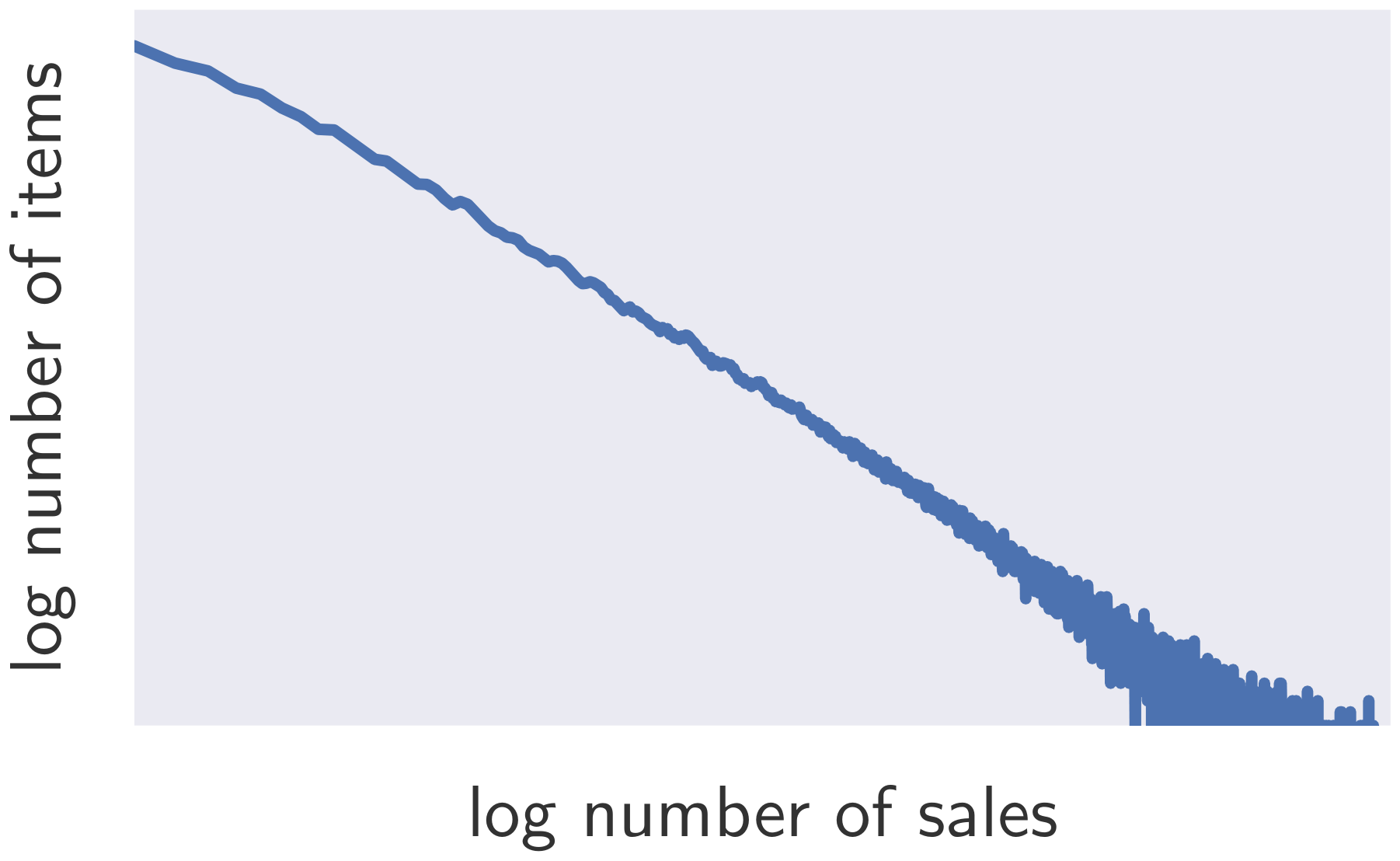
which shows the distribution of sales velocity (i.e. average weekly sales of an item) across millions of items sold by Amazon. The distribution is over a few orders of magnitude an approximate power-law. This observation is to the best of our knowledge new (although maybe not surprising) and has fundamental implications for forecasting methods that attempt to learn global models from such datasets. The scale-free nature of the distribution makes it difficult to divide the data set into sub-groups of time series with a certain velocity band and learn separate models for them, as each such velocity sub-group would have a similar skew. Further, group-based regularization schemes, such as the one proposed by [8], may fail, as the velocities will be vastly different within each group. Finally, such skewed distributions make the use of certain commonly employed normalization techniques, such input standardization or batch normalization [9], less effective.

The main contributions of the paper are twofold: (1) we propose an RNN architecture for probabilistic forecasting, incorporating a negative Binomial likelihood for count data as well as special treatment for the case when the magnitudes of the time series vary widely; (2) we demonstrate empirically on several real-world data sets that this model produces accurate probabilistic forecasts across a range of input characteristics, thus showing that modern deep learning-based approaches can effective address the probabilistic forecasting problem, which is in contrast to common belief in the field and the mixed results reported in ([10, 11]).

In addition to providing better forecast accuracy than previous methods, our approach has a number key advantages compared to classical approaches and other global methods: (i) As the model learns seasonal behavior and dependencies on given covariates across time series, minimal manual feature engineering is needed to capture complex, group-dependent behavior; (ii) DeepAR makes probabilistic forecasts in the form of Monte Carlo samples that can be used to compute consistent quantile estimates for all sub-ranges in the prediction horizon; (iii) By learning from similar items, our method is able to provide forecasts for items with little or no history at all, a case where traditional single-item forecasting methods fail; (vi) Our approach does not assume Gaussian noise, but can incorporate a wide range of likelihood functions, allowing the user to choose one that is appropriate for the statistical properties of the data.

Points (i) and (iii) are what set DeepAR apart from classical forecasting approaches, while (ii) and (iv) pertain to producing accurate, calibrated forecast distributions learned from the historical behavior of all of the time series jointly, which is not addressed by other global methods (see Section 2). Such probabilistic forecasts are of crucial importance in many applications, as they—in contrast to point forecasts—enable optimal decision making under uncertainty by minimizing risk functions, i.e. expectations of some loss function under the forecast distribution.

2. Related Work

Section Summary: Traditional forecasting methods like ARIMA and exponential smoothing often fail on the erratic or intermittent data common in demand forecasting, leading researchers to adopt specialized probability distributions such as the negative binomial to better model such patterns. To improve accuracy, some approaches share information across multiple related time series through techniques like matrix factorization or hierarchical Bayesian priors. Neural networks have long been explored for forecasting but are typically trained separately on each series, in contrast to their successful use in other fields; the probabilistic forecasting setting adds further needs for full predictive distributions and tailored likelihoods for count data.

Due to the immense practical importance of forecasting, a vast variety of different forecasting methods have been developed. Prominent examples of methods for forecasting individual time series include ARIMA models [2] and exponential smoothing methods; [3] provide a unifying review of these and related techniques.

Especially in the demand forecasting domain, one is often faced with highly erratic, intermittent or bursty data which violate core assumptions of many classical techniques, such as Gaussian errors, stationarity, or homoscedasticity of the time series. Since data preprocessing methods (e.g. [12]) often do not alleviate these conditions, forecasting methods have also incorporated more suitable likelihood functions, such as the zero-inflated Poisson distribution, the negative binomial distribution [13], a combination of both [8], or a tailored multi-stage likelihood [4].

Sharing information across time series can improve the forecast accuracy, but is difficult to accomplish in practice, because of the often heterogeneous nature of the data. Matrix factorization methods (e.g. the recent work of [14]), as well as Bayesian methods that share information via hierarchical priors [8] have been proposed as mechanisms for learning across multiple related time series and leveraging hierarchical structure [15].

Neural networks have been investigated in the context of forecasting for a long time (see e.g. the numerous references in the survey [10], or [16] for more recent work considering LSTM cells). More recently, [11] applied neural networks specifically to intermittent data but obtained mixed results. Neural networks in forecasting have been typically applied to individual time series, i.e. a different model is fitted to each time series independently [17, 18, 19]. On the other hand, outside of the forecasting community, time series models based on recurrent neural networks have been very successfully applied to other applications, such as natural language processing [5, 6], audio modeling [7] or image generation [20]. Two main characteristics make the forecasting setting that we consider here different: First, in probabilistic forecasting one is interested in the full predictive distribution, not just a single best realization, to be used in downstream decision making systems. Second, to obtain accurate distributions for (unbounded) count data, we use a negative Binomial likelihood, which improves accuracy but precludes us from directly applying standard data normalization techniques.

3. Model

Section Summary: The model aims to capture the conditional probability distribution of future values in a time series, given its observed history and known external covariates, by factorizing this distribution into a sequence of conditional likelihoods. It employs an autoregressive recurrent neural network with LSTM units that processes previous observations and covariates at each step to output the parameters of a probability distribution (such as Gaussian or negative binomial) from which the next value is drawn. During training the network learns by maximizing the likelihood of observed data, while predictions are generated by sampling multiple possible future trajectories and feeding each sample back as input for the subsequent step.

Denoting the value of time series $i$ at time $t$ by $z_{i, t}$, our goal is to model the conditional distribution

$ P(\mathbf{z}{i, t_0:T} | \mathbf{z}{i, 1:t_0-1}, \mathbf{x}_{i, 1:T})\tag{1} $

of the future of each time series $[z_{i, t_0}, z_{i, t_0 + 1}, \ldots, z_{i, T}] := \mathbf{z}{i, t_0:T}$ given its hboxpast $[z{i, 1}, \ldots, z_{i, t_0-2}, z_{i, t_0-1}] := \mathbf{z}{i, 1:t_0-1}$, where $t_0$ denotes the time point from which we assume $z{i, t}$ to be unknown at prediction time, and $\mathbf{x}{i, 1:T}$ are covariates that are assumed to be known for all time points. To prevent confusion we avoid the ambiguous terms "past" and "future" and will refer to time ranges $[1, t_0-1]$ and $[t_0, T]$ as the conditioning range and prediction range, respectively. During training, both ranges have to lie in the past so that the $z{i, t}$ are observed, but during prediction $z_{i, t}$ is only available in the conditioning range. Note that the time index $t$ is relative, i.e. $t=1$ can correspond to a different actual time period for each $i$.

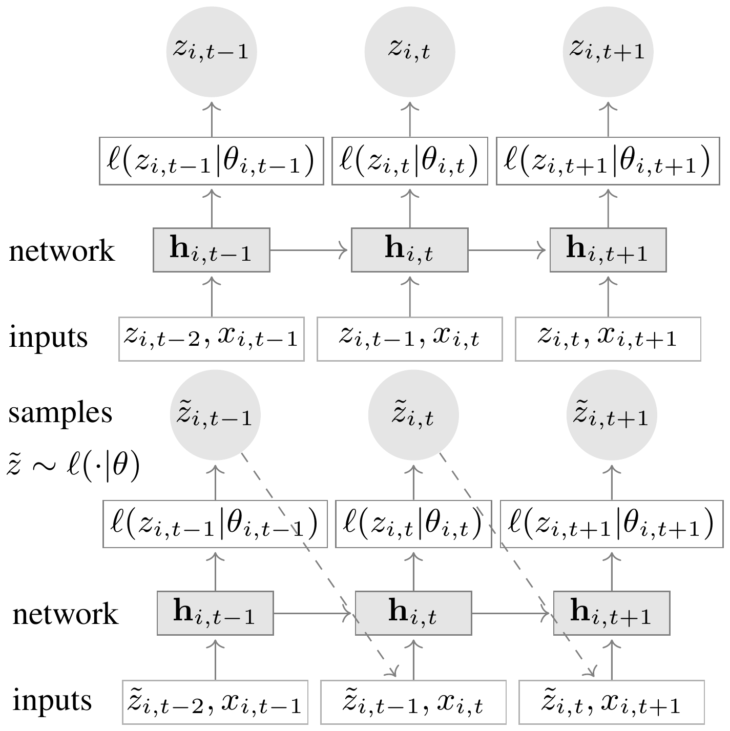
Our model, summarized in Figure 2, is based on an autoregressive recurrent network architecture [5, 6]. We assume that our model distribution $Q_\Theta(\mathbf{z}{i, t_0:T} | \mathbf{z}{i, 1:t_0-1}, \mathbf{x}_{i, 1:T})$ consists of a product of likelihood factors

$ \begin{aligned} Q_\Theta(\mathbf{z}{i, t_0:T} | \mathbf{z}{i, 1:t_0-1}, \mathbf{x}{i, 1:T}) &= \prod\nolimits{t=t_0}^T Q_\Theta(z_{i, t}|\mathbf{z}{i, 1:t-1}, \mathbf{x}{i, 1:T}) = \prod\nolimits_{t=t_0}^T \ell(z_{i, t} | \theta(\mathbf{h}_{i, t}, \Theta)) \end{aligned} $

parametrized by the output $\mathbf{h}_{i, t}$ of an autoregressive recurrent network

$ \mathbf{h}{i, t} = h\left(\mathbf{h}{i, t-1}, z_{i, t-1}, \mathbf{x}_{i, t}, \Theta\right) , ,\tag{2} $

where $h$ is a function implemented by a multi-layer recurrent neural network with LSTM cells. [^1] The model is autoregressive, in the sense that it consumes the observation at the last time step $z_{i, t-1}$ as an input, as well as recurrent, i.e. the previous output of the network $\mathbf{h}{i, t-1}$ is fed back as an input at the next time step. The likelihood $\ell(z{i, t}|\theta(\mathbf{h}{i, t}))$ is a fixed distribution whose parameters are given by a function $\theta(\mathbf{h}{i, t}, \Theta)$ of the network output $\mathbf{h}_{i, t}$ (see below).

[^1]: Details of the architecture and hyper-parameters are given in the supplementary material.

Information about the observations in the conditioning range $\mathbf{z}{i, 1:t_0 -1}$ is transferred to the prediction range through the initial state $\mathbf{h}{i, t_0-1}$. In the sequence-to-sequence setup, this initial state is the output of an encoder network. While in general this encoder network can have a different architecture, in our experiments we opt for using the same architecture for the model in the conditioning range and the prediction range (corresponding to the encoder and decoder in a sequence-to-sequence model). Further, we share weights between them, so that the initial state for the decoder $\mathbf{h}{i, t_0 - 1}$ is obtained by computing Equation 2 for $t = 1, \ldots, t_0 - 1$, where all required quantities are observed. The initial state of the encoder $\mathbf{h}{i, 0}$ as well as $z_{i, 0}$ are initialized to zero.

Given the model parameters $\Theta$, we can directly obtain joint samples $\tilde{\mathbf{z}}{i, t_0:T} \sim Q\Theta(\mathbf{z}{i, t_0:T} | \mathbf{z}{i, 1:t_0-1}, \mathbf{x}{i, 1:T})$ through ancestral sampling: First, we obtain $\mathbf{h}{i, t_0-1}$ by computing Equation 2 for $t=1, \ldots, t_0$. For $t=t_0, t_0+1, \ldots, T$ we sample $\tilde{z}{i, t} \sim \ell(\cdot | \theta(\tilde{\mathbf{h}}{i, t}, \Theta))$ where $\tilde{\mathbf{h}}{i, t} = h\left(\mathbf{h}{i, t-1}, \tilde{z}{i, t-1}, \mathbf{x}{i, t}, \Theta\right)$ initialized with $\tilde{\mathbf{h}}{i, t_0-1} = \mathbf{h}{i, t_0-1}$ and $\tilde{z}{i, t_0 -1} = z{i, t_0 - 1}$. Samples from the model obtained in this way can then be used to compute quantities of interest, e.g. quantiles of the distribution of the sum of values for some time range in the future.

3.1 Likelihood model

The likelihood $\ell(z|\theta)$ determines the "noise model", and should be chosen to match the statistical properties of the data. In our approach, the network directly predicts all parameters $\theta$ (e.g. mean and variance) of the probability distribution for the next time point.

For the experiments in this paper, we consider two choices, Gaussian likelihood for real-valued data, and negative-binomial likelihood for positive count data. Other likelihood models can also readily be used, e.g. beta likelihood for data in the unit interval, Bernoulli likelihood for binary data, or mixtures in order to handle complex marginal distributions, as long as samples from the distribution can cheaply be obtained, and the log-likelihood and its gradients wrt. the parameters can be evaluated. We parametrize the Gaussian likelihood using its mean and standard deviation, $\theta = (\mu, \sigma)$, where the mean is given by an affine function of the network output, and the standard deviation is obtained by applying an affine transformation followed by a softplus activation in order to ensure $\sigma > 0$:

$ \begin{aligned} \ell_\text{G}(z|\mu, \sigma) &= (2\pi\sigma^2)^{-\frac{1}{2}}\exp(-(z - \mu)^2/(2\sigma^2))\ \mu(\mathbf{h}{i, t}) &= \mathbf{w}\mu^T \mathbf{h}{i, t} + b\mu \quad\text{and}\quad \sigma(\mathbf{h}{i, t}) = \log(1 + \exp(\mathbf{w}\sigma^T \mathbf{h}{i, t} + b\sigma)) ;. \end{aligned} $

For modeling time series of positive count data, the negative binomial distribution is a commonly used choice [13, 8]. We parameterize the negative binomial distribution by its mean $\mu \in \mathbb{R}^+$ and a shape parameter $\alpha \in \mathbb{R}^+$,

$ \begin{aligned} \ell_{\text{NB}}(z|\mu, \alpha) &= \frac{\Gamma(z + \frac{1}{\alpha})}{\Gamma(z + 1)\Gamma(\frac{1}{\alpha})} \left(\frac{1}{1 + \alpha \mu}\right)^\frac{1}{\alpha} \left(\frac{\alpha \mu}{1 + \alpha \mu}\right)^z \ \mu(\mathbf{h}{i, t}) &= \log(1 + \exp(\mathbf{w}\mu^T \mathbf{h}{i, t} + b\mu)) \quad\text{and}\quad \alpha(\mathbf{h}{i, t}) = \log(1 + \exp(\mathbf{w}\alpha^T \mathbf{h}{i, t} + b\alpha)) ;, \end{aligned} $

where both parameters are obtained from the network output by a fully-connected layer with softplus activation to ensure positivity. In this parameterization of the negative binomial distribution the shape parameter $\alpha$ scales the variance relative to the mean, i.e. $\text{Var}[z] = \mu + \mu^2 \alpha$. While other parameterizations are possible, we found this particular one to be especially conducive to fast convergence in preliminary experiments.

3.2 Training

Given a data set of time series ${\mathbf{z}{i, 1:T}}{i = 1, \ldots, N}$ and associated covariates $\mathbf{x}{i, 1:T}$, obtained by choosing a time range such that $z{i, t}$ in the prediction range is known, the parameters $\Theta$ of the model, consisting of the parameters of the RNN $h(\cdot)$ as well as the parameters of $\theta(\cdot)$, can be learned by maximizing the hboxlog-likelihood

$ \mathcal{L} = \sum_{i=1}^{N} \sum_{t=t_0}^{T} \log \ell(z_{i, t}|\theta(\mathbf{h}_{i, t})), .\tag{3} $

As $\mathbf{h}_{i, t}$ is a deterministic function of the input, all quantities required to compute Equation 3 are observed, so that—in contrast to state space models with latent variables—no inference is required, and 3 can be optimized directly via stochastic gradient descent by computing gradients with respect to $\Theta$. In our experiments, where the encoder model is the same as the decoder, the distinction between encoder and decoder is somewhat artificial during training, so that we also include the likelihood terms for $t=0, \ldots, t_0 - 1$ in Equation 3 (or, equivalently, set $t_0 = 0$).

For each time series in the dataset, we generate multiple training instances by selecting windows with different starting points from the original time series. In practice, we keep the total length $T$ as well as the relative length of the conditioning and prediction ranges fixed for all training examples. For example, if the total available range for a given time series ranges from 2013-01-01 to 2017-01-01, we can create training examples with $t=1$ corresponding to 2013-01-01, 2013-01-02, 2013-01-03, and so on. When choosing these windows we ensure that entire prediction range is always covered by the available ground truth data, but we may chose $t=1$ to lie before the start of the time series, e.g. 2012-12-01 in the example above, padding the unobserved target with zeros. This allows the model to learn the behavior of "new" time series taking into account all other available features. By augmenting the data using this windowing procedure, we ensure that information about absolute time is only available to the model through covariates, but not through the relative position of $z_{i, t}$ in the time series.

[21] noted that, due to the autoregressive nature of such models, optimizing Equation 3 directly causes a discrepancy between how the model is used during training and when obtaining predictions from the model: during training, the values of $z_{i, t}$ are known in the prediction range and can be used to compute $\mathbf{h}{i, t}$; during prediction however, $z{i, t}$ is unknown for $t \geq t_0$, and a single sample $\tilde{z}{i, t} \sim \ell(\cdot| \theta(\mathbf{h}{i, t}))$ from the model distribution is used in the computation of $\mathbf{h}_{i, t}$ according to 2 instead. While it has been shown that this disconnect poses a severe problem for e.g. NLP tasks, we have not observed adverse effects from this in the forecasting setting. Preliminary experiments with variants of scheduled sampling ([21]) did not show any significant accuracy improvements (but slowed convergence).

3.3 Scale handling

Applying the model to data that exhibits a power-law of scales as depicted in Figure 1 presents two challenges. Firstly, due to the autoregressive nature of the model, both the autoregressive input $z_{i, t-1}$ as well as the output of the network (e.g.\ $\mu$) directly scale with the observations $z_{i, t}$, but the non-linearities of the network in between have a limited operating range. Without further modifications, the network thus has to learn to scale the input to an appropriate range in the input layer, and then to invert this scaling at the output. We address this issue by dividing the autoregressive inputs $z_{i, t}$ (or $\tilde{z}{i, t}$) by an item-dependent scale factor $\nu_i$, and conversely multiplying the scale-dependent likelihood parameters by the same factor. For instance, for the negative binomial likelihood we use $\mu=\nu_i \log(1 + \exp(o\mu))$ and $\alpha = \log(1 + \exp(o_\alpha))/\sqrt{\nu_i}$ where $o_\mu$, $o_\alpha$ are the outputs of the network for these parameters. Note that while for real-valued data one could alternatively scale the input in a preprocessing step, this is not possible for count distributions. Choosing an appropriate scale factor might in itself be challenging (especially in the presence of missing data or large within-item variances). However, scaling by the average value $\nu_i = 1 + \frac{1}{t_0} \sum_{t=1}^{t_0} z_{i, t}$, as we do in our experiments, is a heuristic that works well in practice.

Secondly, due to the imbalance in the data, a stochastic optimization procedure that picks training instances uniformly at random will visit the small number time series with a large scale very infrequently, which result in underfitting those time series. This could be especially problematic in the demand forecasting setting, where high-velocity items can exhibit qualitatively different behavior than low-velocity items, and having an accurate forecast for high-velocity items might be more important for meeting certain business objectives. To counteract this effect, we sample the examples non-uniformly during training. In particular, in our weighted sampling scheme, the probability of selecting a window from an example with scale $\nu_i$ is proportional to $\nu_i$. This sampling scheme is simple, yet effectively compensates for the skew in Figure 1.

3.4 Features

The covariates $\mathbf{x}_{i, t}$ can be item-dependent, time-dependent, or both. [^2] They can be used to provide additional information about the item or the time point (e.g. week of year) to the model. They can also be used to include covariates that one expects to influence the outcome (e.g. price or promotion status in the demand forecasting setting), as long as the features' values are available also in the prediction range.

[^2]: Covariates $\mathbf{x}_{i, t}$ that do not depend on time are handled by repeating them along the time dimension.

In all experiments we use an "age" feature, i.e., the distance to the first observation in that time series. We also add day-of-the-week and hour-of-the-day for hourly data, week-of-year for weekly data and month-of-year for monthly data. [^3] Further, we include a single categorical item feature, for which an embedding is learned by the model. In the retail demand forecasting data sets, the item feature corresponds to a (coarse) product category (e.g. "clothing"), while in the smaller data sets it corresponds to the item's identity, allowing the model to learn item-specific behavior. We standardize all covariates to have zero mean and unit variance.

[^3]: Instead of using dummy variables to encode these, we simply encode them as increasing numeric values.

4. Applications and Experiments

Section Summary: The authors implemented their forecasting model in MXNet and ran all experiments on modest cloud hardware, completing full training and prediction on a half-million time series dataset in under ten hours. They evaluated the approach on five real-world collections of time series—monthly auto parts sales, hourly electricity usage, freeway traffic occupancy, and two large Amazon item-sales datasets—comparing accuracy and uncertainty calibration against established baselines such as Croston’s method and state-space models. Results show that the model matches or exceeds the best prior methods on standard error metrics while producing more realistic, data-driven uncertainty estimates that improve when temporal correlations in the forecasts are preserved.

We implement our model using MXNet, and use a single p2.xlarge AWS instance containing 4 CPUs and 1 GPU to run all experiments. On this hardware, a full training & prediction run on the large ec dataset containing 500K time series can be completed in less than 10 hours. While prediction is already fast, is can easily parallelized if necessary. A description of the (simple) hyper-parameter tuning procedure, the obtained hyper-parameter values, as well as statistics of datasets and running time are given in supplementary material.

Datasets – We use five datasets for our evaluations. The first three–parts, electricity, and traffic–are public datasets; parts consists of 1046 aligned time series of 50 time steps each, representing monthly sales for different items of a US automobile company [4]; electricity contains hourly time series of the electricity consumption of 370 customers [14]; traffic, also used in [14], contains the hourly occupancy rate, between 0 and 1, of 963 car lanes of San Francisco bay area freeways. For the parts dataset, we use the 42 first months as training data and report error on the remaining 8. For electricity we train with data between 2014-01-01 and 2014-09-01, for traffic we train all the data available before 2008-06-15. The results for electricity and traffic are computed using rolling window predictions done after the last point seen in training as described in [14]. We do not retrain our model for each window, but use a single model trained on the data before the first prediction window. The remaining two datasets ec and ec-sub are weekly item sales from Amazon used in [4]. We predict 52 weeks and evaluation is done on the year following 2014-09-07. The time series in these two datasets are very diverse and erratic, ranging from very fast to very slow moving items, and contains "new" products introduced in the weeks before the forecast time 2014-09-07, see Figure 3. Further, item velocities in this data set have a power-law distribution, as shown in Figure 1.

\begin{tabular}{l|rrrrrrrrr}
\toprule
 {} & \multicolumn{4}{c}{$0.5$-risk} & \multicolumn{4}{c}{$0.9$-risk} & average \\
\midrule
 {} & \multicolumn{9}{c}{\texttt{parts}} \\
$(L, S)$ & $(0, 1)$ & $(2, 1)$ & $(0, 8)$ & all(8) & $(0, 1)$ & $(2, 1)$ & $(0, 8)$ & all(8) & average\\
\midrule
\texttt{Snyder} (baseline) & 1.00 & 1.00 & 1.00 & \bf{1.00} & 1.00 & 1.00 & 1.00 & 1.00 & 1.00 \\
\texttt{Croston} & 1.47 & 1.70 & 2.86 & 1.83 & - & - & - & - & 1.97 \\
\texttt{ISSM} & 1.04 & 1.07 & 1.24 & 1.06 & 1.01 & 1.03 & 1.14 & 1.06 & 1.08 \\
\texttt{ETS} & 1.28 & 1.33 & 1.42 & 1.38 & 1.01 & 1.03 & 1.35 & 1.04 & 1.23 \\
\texttt{rnn-gaussian} & 1.17 & 1.49 & 1.15 & 1.56 & 1.02 & 0.98 & 1.12 & 1.04 & 1.19 \\
\texttt{rnn-negbin} & \bf{0.95} & \bf{0.91} & 0.95 & \bf{1.00} & 1.10 & \bf{0.95} & 1.06 & 0.99 & 0.99 \\
\texttt{DeepAR} & 0.98 & \bf{0.91} & \bf{0.91} & 1.01 & \bf{0.90} & \bf{0.95} & \bf{0.96} & \bf{0.94} & \bf{0.94} \\
\midrule
 {} & \multicolumn{9}{c}{\texttt{ec-sub}} \\
  $(L, S)$ & $(0, 2)$ & $(0, 8)$ & (3, 12) & all(33) & $(0, 2)$ & $(0, 8)$ & (3, 12) & all(33) & average\\
\midrule
\texttt{Snyder} & 1.04 & 1.18 & 1.18 & 1.07 & 1.0 & 1.25 & 1.37 & 1.17 & 1.16 \\
\texttt{Croston} & 1.29 & 1.36 & 1.26 & 0.88 & - & - & - & - & 1.20 \\
\texttt{ISSM} (baseline) & 1.00 & 1.00 & 1.00 & 1.00 & 1.00 & 1.00 & \bf{1.00} & 1.00 & 1.00 \\
\texttt{ETS} & 0.83 & 1.06 & 1.15 & 0.84 & 1.09 & 1.38 & 1.45 & 0.74 & 1.07 \\
\texttt{rnn-gaussian} & 1.03 & 1.19 & 1.24 & 0.85 & 0.91 & 1.74 & 2.09 & 0.67 & 1.21\\
\texttt{rnn-negbin} & 0.90 & 0.98 & 1.11 & 0.85 & 1.23 & 1.67 & 1.83 & 0.78 & 1.17 \\
\texttt{DeepAR} & \bf{0.64} & \bf{0.74} & \bf{0.93} & \bf{0.73} & \bf{0.71} & \bf{0.81} & 1.03 & \bf{0.57} & \bf{0.77} \\
\midrule
 {} & \multicolumn{9}{c}{\texttt{ec}} \\
$(L, S)$ & $(0, 2)$ & $(0, 8)$ & (3, 12) & all(33) & $(0, 2)$ & $(0, 8)$ & (3, 12) & all(33) & average\\
\midrule
\texttt{Snyder} & 0.87 & 1.06 & 1.16 & 1.12 & 0.94 & 1.09 & 1.13 & 1.01 & 1.05 \\
\texttt{Croston} & 1.30 & 1.38 & 1.28 & 1.39 & - & - & - & - & 1.34 \\
\texttt{ISSM} (baseline) & 1.00 & 1.00 & 1.00 & 1.00 & 1.00 & 1.00 & \bf{1.00} & 1.00 & 1.00 \\
\texttt{ETS} & 0.77 & 0.97 & 1.07 & 1.23 & 1.05 & 1.33 & 1.37 & 1.11 & 1.11 \\
\texttt{rnn-gaussian} & 0.89 & 0.91 & 0.94 & 1.14 & 0.90 & 1.15 & 1.23 & \bf{0.90} & 1.01 \\
\texttt{rnn-negbin} & 0.66 & 0.71 & \bf{0.86} & \bf{0.92} & 0.85 & 1.12 & 1.33 & 0.98 & 0.93 \\
\texttt{DeepAR} & \bf{0.59} & \bf{0.68} & 0.99 & 0.98 & \bf{0.76} & \bf{0.88} & \bf{1.00} & 0.91 & \bf{0.85} \\
\bottomrule
\end{tabular}

4.1 Accuracy comparison

For the parts and ec/ec-sub datasets we compare with the following baselines which represent the state-of-the-art on demand integer datasets to the best of our knowledge:

• Croston: the Croston method developed for intermittent demand forecasting from R package ([22])
• ETS: the ETS model ([3]) from R package with automatic model selection. Only additive models are used as multiplicative models shows numerical issues on some time series.
• Snyder the negative-binomial autoregressive method of ([13])
• ISSM the method of ([4]) using an innovative state space model with covariates features

In addition, we compare to two baseline RNN models to see the effect of our contributions:

• rnn-gaussian uses the same architecture as DeepAR with a Gaussian likelihood; however, it uses uniform sampling, and a simpler scaling mechanism, where time series $z_i$ are divided by $\nu_i$ and outputs are multiplied by $\nu_i$
• rnn-negbin uses a negative binomial distribution, but does not scale inputs and outputs of the RNN and training instances are drawn uniformly rather than using weighted sampling.

As in ([4]), we use $\rho$-risk metrics (quantile loss) that quantify the accuracy of a quantile $\rho$ of the predictive distribution; the exact definition of these metric is given in supplementary material. The metrics are evaluated for a certain spans $[L, L+S)$ in the prediction range, where $L$ is a lead time after the forecast start point. Table 1 shows the $0.5$-risk and $0.9$-risk and for different lead times and spans. Here all(K) denotes the average risk of the marginals $[L, L+1)$ for $L<K$. We normalize all reported metrics with respect to the strongest previously published method (baseline). DeepAR performs significantly better than all other methods on these datasets. The results also show the importance of modeling these data sets with a count distribution, as rnn-gaussian performs significantly worse. The ec and ec-sub data sets exhibit the power law behavior discussed above, and without scaling and weighted sampling accuracy is decreased (rnn-negbin). On the parts data set, which does not exhibit the power-law behavior, rnn-negbin performs similar to DeepAR.

```latextable {caption="Table 2: Comparison with MatFact"} \begin{tabular}{l|rrrrr} \toprule {} & \multicolumn{2}{c}{\texttt{electricity}} & \multicolumn{2}{c}{\texttt{traffic}} \ {} & ND & RMSE & ND & RMSE \ \midrule \texttt{MatFact} & 0.16 & 1.15 & 0.20 & 0.43 \ \texttt{DeepAR} & \bf{0.07} & \bf{1.00} & \bf{0.17} & \bf{0.42} \ \bottomrule \end{tabular}

In Table 2 we compare point forecast accuracy on the `electricity` and `traffic` datasets against the matrix factorization technique (`MatFact`) proposed in [14]. We consider the same metrics namely Normalized Deviation (ND) and Normalized RMSE (NRMSE) whose definition are given in the supplementary material. The results show that DeepAR outperforms `MatFact` on both datasets.

### 4.2 Qualitative analysis

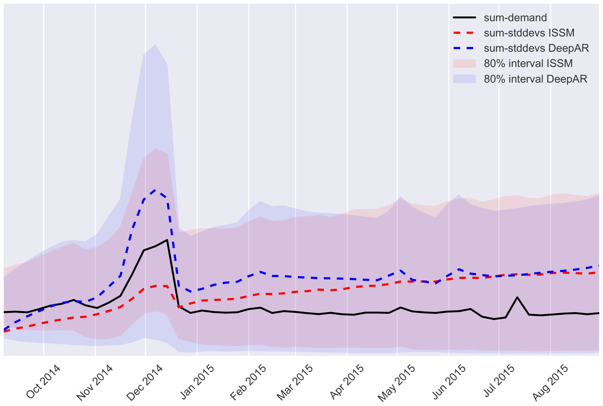
Figure 3 shows example predictions from the `ec` data set. In Figure 4, we show aggregate sums of different quantiles of the marginal predictive distribution for `DeepAR` and `ISSM` on the `ec` dataset. In contrast to ISSM models such as [4], where a linear growth of uncertainty is part of the modeling assumptions, the uncertainty growth pattern is learned from the data. In this case, the model does learn an overall growth of uncertainty over time. However, this is not simply linear growth: uncertainty (correctly) increases during Q4, and decreases again shortly afterwards.

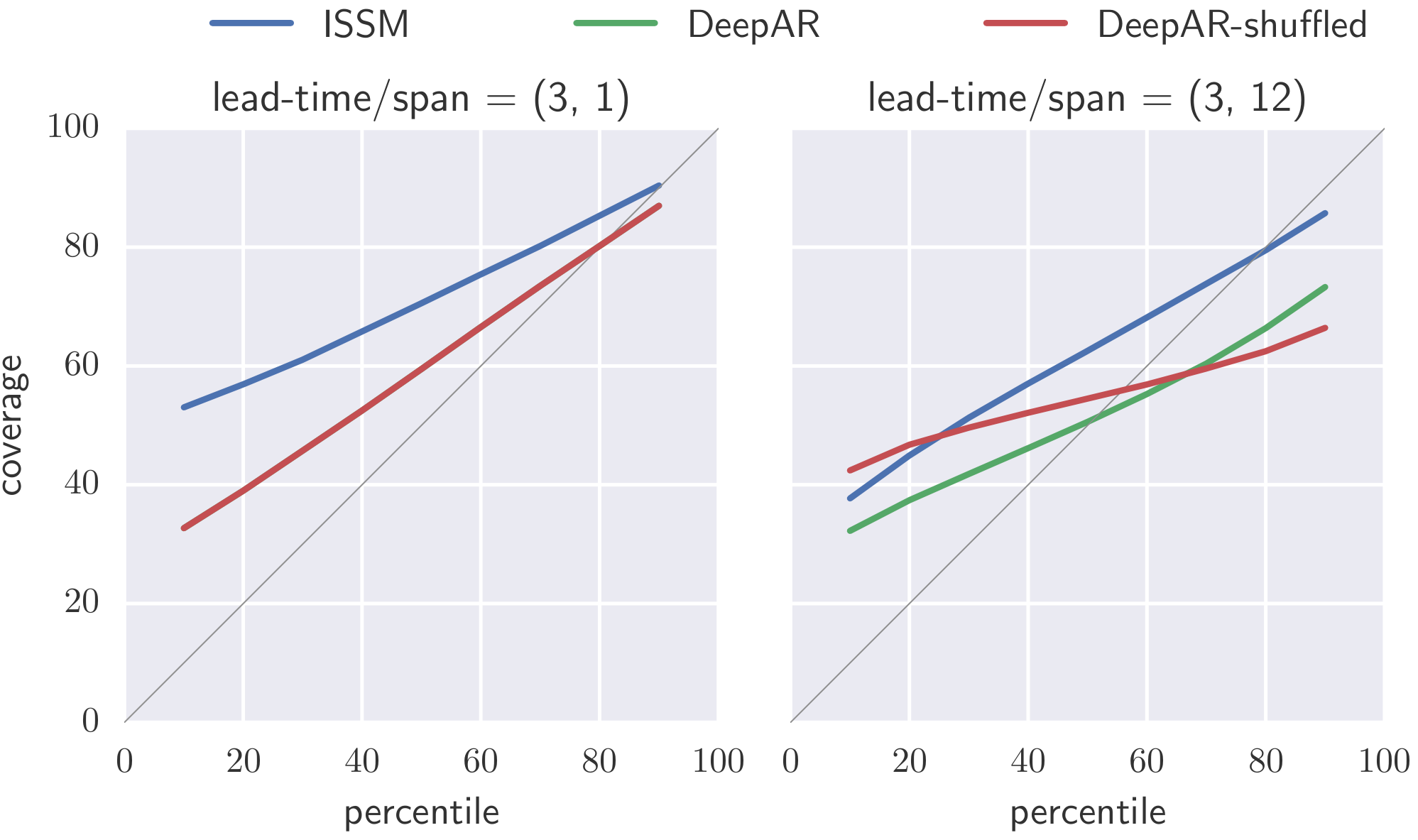
The calibration of the forecast distribution is depicted in Figure 5. Here we show, for each percentile $p$ the $\text{Coverage}(p)$, which is defined as the fraction of time series in the dataset for which the $p$-percentile of the predictive distribution is larger than the the true target. For a perfectly calibrated prediction it holds that $\text{Coverage}(p) = p$, which corresponds to the diagonal. Compared to the `ISSM` model, calibration is improved overall.

To assess the effect of modeling correlations in the output, i.e., how much they differ from independent distributions for each time-point, we plot the calibration curves for a shuffled forecast, where for each time point the realizations of the original forecast have been shuffled, destroying any correlation between time steps. For the short lead-time span (left) which consists of just one time-point, this has no impact, because it is just the marginal distribution. For the longer lead-time span (right), however, destroying the correlation leads to a worse calibration, showing that important temporal correlations are captured between the time steps.

## 5. Conclusion

> **Section Summary**: Recent advances in deep learning have produced forecasting methods that deliver substantially more accurate predictions than traditional approaches across many different datasets. The DeepAR model learns shared patterns from groups of related time series, automatically handles differing scales, and generates reliable probability estimates for future values while capturing features such as seasonality. It achieves these results with little parameter tuning and remains effective even on collections containing only a few hundred series.


We have shown that forecasting approaches based on modern deep learning techniques can drastically improve forecast accuracy over state of the art forecasting methods on a wide variety of data sets. Our proposed DeepAR model effectively learns a *global* model from related time series, handles widely-varying scales through rescaling and velocity-based sampling, generates calibrated probabilistic forecasts with high accuracy, and is able to learn complex patterns such as seasonality and uncertainty growth over time from the data.

Interestingly, the method works with little or no hyperparameter tuning on a wide variety of datasets, and in is applicable to medium-size datasets containing only a few hundred time series.

## 6. Supplementary materials

> **Section Summary**: The supplementary materials define several error metrics for evaluating probabilistic forecasts, including a normalized ρ-risk based on quantile loss, along with ND and RMSE that compare predicted medians against actual values across items and time periods. They also detail the experimental setup, which relies on the MxNet framework with LSTM networks trained via the ADAM optimizer, dataset-specific hyperparameters selected through grid search on held-out training partitions, and end-to-end runtimes measured on standard hardware. Finally, the section explains how missing observations are handled by substituting samples drawn from the model's conditional predictive distribution, preventing systematic biases such as under-forecasting in demand settings where stockouts occur.


### Error metrics

#### $\rho$-risk metric

The aggregated target value of an item $i$ in a span is denoted as $Z_i(L, S) = \sum_{t=t_0+L}^{t_0 + L + S} z_{i, t}$. For a given quantile $\rho\in(0, 1)$ we denote the predicted $\rho$-quantile for $Z_i(L, S)$ by $\hat{Z}^\rho_i(L, S)$. To obtain such a quantile prediction from a set of sample paths, each realization is first summed in the given span. The samples of these sums then represent the estimated distribution for $Z_i(L, S)$ and we can take the $\rho$-quantile from the empirical distribution.

The $\rho$-quantile loss is then defined as

$
L_{\rho}(Z, \hat{Z}^\rho) = 2 (\hat{Z} - Z)\left(\rho \mathrm{I}_{\hat{Z}^\rho>Z} - (1 - \rho) \mathrm{I}_{\hat{Z}^\rho \leq Z}\right) \;.
$

In order to summarize the quantile losses for a given span across all items, we consider a normalized sum of quantile losses $\left(\sum_i L_\rho(Z_i, \hat{Z}_i^\rho\right) / \left(\sum_i Z_i\right)$, which we call the $\rho$-risk.

#### ND and RMSE metrics

ND and RMSE metrics are defined as follow:

$
\begin{aligned}
\text{ND} &= \frac{\sum_{i, t} |z_{i, t} - \hat{z}_{i, t}|}{\sum_{i, t} |z_{i, t}|} &
 \text{RMSE} &= \frac{\sqrt{\frac{1}{N (T - t_0)}\sum_{i, t}(z_{i, t} - \hat{z}_{i, t})^2}}{\frac{1}{N (T - t_0)}\sum_{i, t} |z_{i, t}|}
\end{aligned}
$

where $\hat{z}_{i, t}$ is the predicted median value for item $i$ at time $t$ and the sums are over all items and all time points in the prediction period.

### Experiment details

We use MxNet as our neural network framework [23]. Experiments are run on a laptop for `parts` and with a single AWS p2.xlarge instance (four core machine with a single GPU) for other datasets. Note that predictions can be done in all datasets end to end in a matter of hours even with a single machine. We use ADAM optimizer [24] with early stopping and standard LSTM cells with a forget bias set to $1.0$ in all experiment and 200 samples are drawn from our decoder to generate predictions.

```latextable {caption="Table 3: Datasets statistics and RNN parameters"}
\begin{tabular}{cccccc}
\midrule
  {} & \texttt{parts} & \texttt{electricity} & \texttt{traffic} & \texttt{ec-sub} & \texttt{ec} \\\midrule
$#$ time series & 1046 & 370 & 963 & 39700 & 534884 \\
time granularity & month & hourly & hourly & week & week \\
domain& $\mathbb{N}$ & $\mathbb{R}^+$ & $[0, 1]$ & $\mathbb{N}$ & $\mathbb{N}$ \\
encoder length & 8 & 168 & 168 & 52 & 52 \\
decoder length & 8 & 24 & 24 & 52 & 52 \\
$#$ training examples & 35K & 500K & 500K & 2M & 2M \\
item input embedding dimension & 1046 & 370 & 963 & 5 & 5 \\
item output embedding dimension & 1 & 20 & 20 & 20 & 20 \\
batch size & 64 & 64 & 64 & 512 & 512 \\
learning rate & 1e-3 & 1e-3 & 1e-3 & 5e-3 & 5e-3 \\
$#$ LSTM layers & 3 & 3 & 3 & 3 & 3 \\
$#$ LSTM nodes & 40 & 40 & 40 & 120 & 120 \\
running time & 5min & 7h & 3h & 3h & 10h \\
\midrule
\end{tabular}

For parts dataset, we use the 42 first months as training data and report error on the remaining 8. For the other datasets electricity, traffic, ec-sub and ec the set of possible training instances is sub-sampled to the number indicated in Table 3. The scores of electricity and traffic are reported using the rolling window operation described in [14], note that we do not retrain our model but reuse the same one for predicting across the different time windows instead. Running times measures an end to end evaluation, e.g. processing features, training the neural network, drawing samples and evaluating produced distributions.

For each dataset, a grid-search is used to find the best value for the hyper-parameters item output embedding dimension and # LSTM nodes (e.g. hidden number of units). To do so, the data before the forecast start time is used as training set and split into two partitions. For each hyper-parameter candidate, we fit our model on the first partition of the training set containing 90% of the data and we pick the one that has the minimal negative log-likelihood on the remaining 10%. Once the best set of hyper-parameters is found, the evaluation metrics (0.5-risk, 0.9-risk, ND and RMSE) are then evaluated on the test set, e.g. the data coming after the forecast start time. Note that this procedure could lead to over-fitting the hyper-parameters to the training set but this would then also degrades the metric we report. A better procedure would be to fit parameters and evaluate negative log-likelihood not only on different windows but also on non-overlapping time intervals. As for the learning rate, it is tuned manually for every dataset and is kept fixed in hyper-parameter tuning. Other parameters such as encoder length, decoder length and item input embedding are considered domain dependent and are not fitted. Batch size is increased on larger datasets to benefit more from GPU's parallelization. Finally, running times measures an end to end evaluation, e.g. processing features, training the neural network, drawing samples and evaluating produced distributions.

Missing Observations

In some forecasting settings, the target values $z_{i, t}$ might be missing (or unobserved) for a subset of the time points. For instance, in the context of demand forecasting, an item may be out-of-stock at a certain time, in which case the demand for the item cannot be observed. Not explicitly modeling such missing observations (e.g. by assuming that the observed sales correspond to the demand even when an item is out of stock), can, in the best case, lead to systematic forecast underbias, and, in a worst case in the larger supply chain context, can lead to a disastrous downward spiral where an out-of-stock situation leads to a lower demand forecast, lower re-ordering and more out-of-stock-situations. In our model, missing observations can easily be handled in a principled way by replacing each unobserved value $z_{i, t}$ by a sample $\tilde{z}{i, t} \sim \ell(\cdot|\theta(\mathbf{h}{i, t}))$ from the conditional predictive distribution when computing (1), and excluding the likelihood term corresponding to the missing observation from (2). We omitted experimental results in this setting from the paper, as doing a proper evaluation in the light of missing data in the prediction range requires non-standard adjusted metrics that are hard to compare across studies (see e.g. ([4])).

References

Section Summary: This section compiles academic citations on supply chain management, statistical forecasting methods such as exponential smoothing and ARIMA models, and machine learning techniques for time series data. The references prominently feature works on neural networks, including recurrent models like LSTMs and sequence-to-sequence architectures, along with their use in demand prediction and inventory applications. Additional entries address optimization tools, data transformations, and empirical studies comparing traditional and deep learning approaches.

[1] Paul D. Larson, David Simchi-Levi, Philip Kaminsky, and Edith Simchi-Levi. Designing and managing the supply chain: Concepts, strategies, and case studies. Journal of Business Logistics, 22(1):259–261, 2001. ISSN 2158-1592. doi:10.1002/j.2158-1592.2001.tb00165.x. URL http://dx.doi.org/10.1002/j.2158-1592.2001.tb00165.x.

[2] George E. P. Box and Gwilym M. Jenkins. Some recent advances in forecasting and control. Journal of the Royal Statistical Society. Series C (Applied Statistics), 17(2):91–109, 1968.

[3] R. Hyndman, A. B. Koehler, J. K. Ord, and R .D. Snyder. Forecasting with Exponential Smoothing: The State Space Approach. Springer Series in Statistics. Springer, 2008. ISBN 9783540719182.

[4] Matthias W Seeger, David Salinas, and Valentin Flunkert. Bayesian intermittent demand forecasting for large inventories. In Advances in Neural Information Processing Systems, pages 4646–4654, 2016.

[5] Alex Graves. Generating sequences with recurrent neural networks. arXiv preprint arXiv:1308.0850, 2013.

[6] Ilya Sutskever, Oriol Vinyals, and Quoc V Le. Sequence to sequence learning with neural networks. In Advances in Neural Information Processing Systems, pages 3104–3112, 2014.

[7] Aäron van den Oord, Sander Dieleman, Heiga Zen, Karen Simonyan, Oriol Vinyals, Alex Graves, Nal Kalchbrenner, Andrew W. Senior, and Koray Kavukcuoglu. Wavenet: A generative model for raw audio. CoRR, abs/1609.03499, 2016.

[8] Nicolas Chapados. Effective bayesian modeling of groups of related count time series. In Proceedings of The 31st International Conference on Machine Learning, pages 1395–1403, 2014.

[9] Sergey Ioffe and Christian Szegedy. Batch normalization: Accelerating deep network training by reducing internal covariate shift. In Proceedings of the 32nd International Conference on Machine Learning, ICML 2015, Lille, France, 6-11 July 2015, pages 448–456, 2015.

[10] Guoqiang Zhang, B. Eddy Patuwo, and Michael Y. Hu. Forecasting with artificial neural networks:: The state of the art. International Journal of Forecasting, 14(1):35–62, 1998.

[11] Nikolaos Kourentzes. Intermittent demand forecasts with neural networks. International Journal of Production Economics, 143(1):198–206, 2013. ISSN 09255273. doi:10.1016/j.ijpe.2013.01.009.

[12] G. E. P. Box and D. R. Cox. An analysis of transformations. Journal of the Royal Statistical Society. Series B (Methodological), 26(2):211–252, 1964.

[13] Ralph D Snyder, J Keith Ord, and Adrian Beaumont. Forecasting the intermittent demand for slow-moving inventories: A modelling approach. International Journal of Forecasting, 28(2):485–496, 2012.

[14] Hsiang-Fu Yu, Nikhil Rao, and Inderjit S Dhillon. Temporal regularized matrix factorization for high-dimensional time series prediction. In D. D. Lee, M. Sugiyama, U. V. Luxburg, I. Guyon, and R. Garnett, editors, Advances in Neural Information Processing Systems 29, pages 847–855. Curran Associates, Inc., 2016.

[15] Rob J. Hyndman, Roman A. Ahmed, George Athanasopoulos, and Han Lin Shang. Optimal combination forecasts for hierarchical time series. Computational Statistics & Data Analysis, 55(9):2579 – 2589, 2011.

[16] F. A. Gers, D. Eck, and J. Schmidhuber. Applying LSTM to time series predictable through time-window approaches. In Georg Dorffner, editor, Artificial Neural Networks – ICANN 2001 (Proceedings), pages 669–676. Springer, 2001.

[17] Iebeling Kaastra and Milton Boyd. Designing a neural network for forecasting financial and economic time series. Neurocomputing, 10(3):215–236, 1996.

[18] M Ghiassi, H Saidane, and DK Zimbra. A dynamic artificial neural network model for forecasting time series events. International Journal of Forecasting, 21(2):341–362, 2005.

[19] Luis A D'ıaz-Robles, Juan C Ortega, Joshua S Fu, Gregory D Reed, Judith C Chow, John G Watson, and Juan A Moncada-Herrera. A hybrid arima and artificial neural networks model to forecast particulate matter in urban areas: the case of temuco, chile. Atmospheric Environment, 42(35):8331–8340, 2008.

[20] Karol Gregor, Ivo Danihelka, Alex Graves, Danilo Jimenez Rezende, and Daan Wierstra. Draw: A recurrent neural network for image generation. arXiv preprint arXiv:1502.04623, 2015.

[21] Samy Bengio, Oriol Vinyals, Navdeep Jaitly, and Noam Shazeer. Scheduled sampling for sequence prediction with recurrent neural networks. In Advances in Neural Information Processing Systems, pages 1171–1179, 2015.

[22] Rob J Hyndman and Yeasmin Khandakar. Automatic time series forecasting: the forecast package for R. Journal of Statistical Software, 26(3):1–22, 2008. URL http://www.jstatsoft.org/article/view/v027i03.

[23] Tianqi Chen, Mu Li, Yutian Li, Min Lin, Naiyan Wang, Minjie Wang, Tianjun Xiao, Bing Xu, Chiyuan Zhang, and Zheng Zhang. Mxnet: A flexible and efficient machine learning library for heterogeneous distributed systems. CoRR, abs/1512.01274, 2015.

[24] Diederik P. Kingma and Jimmy Ba. Adam: A method for stochastic optimization. CoRR, abs/1412.6980, 2014. URL http://arxiv.org/abs/1412.6980.