Auto-Encoding Variational Bayes
Diederik P. Kingma
Machine Learning Group
Universiteit van Amsterdam[email protected]
Max Welling
Machine Learning Group
Universiteit van Amsterdam[email protected]
Abstract
How can we perform efficient inference and learning in directed probabilistic models, in the presence of continuous latent variables with intractable posterior distributions, and large datasets? We introduce a stochastic variational inference and learning algorithm that scales to large datasets and, under some mild differentiability conditions, even works in the intractable case. Our contributions are two-fold. First, we show that a reparameterization of the variational lower bound yields a lower bound estimator that can be straightforwardly optimized using standard stochastic gradient methods. Second, we show that for i.i.d. datasets with continuous latent variables per datapoint, posterior inference can be made especially efficient by fitting an approximate inference model (also called a recognition model) to the intractable posterior using the proposed lower bound estimator. Theoretical advantages are reflected in experimental results.
Executive Summary: In the field of machine learning, a key challenge arises when modeling complex data like images or faces using probabilistic models that include hidden, continuous variables—such as latent factors representing underlying patterns. These models often have "intractable" posteriors, meaning the math to infer hidden variables from observed data is too complex to compute directly, especially with large datasets. This limits efficient training and inference, hindering applications in generative tasks like creating realistic synthetic images or denoising noisy data. As data volumes grow in areas like computer vision, scalable methods are urgently needed to learn useful representations without prohibitive computation.
This paper aims to develop an efficient algorithm for inference and learning in such directed probabilistic models with continuous latent variables, even when exact computations are impossible. It specifically targets maximum likelihood estimation of model parameters and approximate posterior inference for latent variables, using independent and identically distributed datasets.
The authors propose a high-level approach based on variational Bayesian methods, which approximate intractable probabilities with simpler ones to create a lower bound on the data likelihood. They introduce a "reparameterization trick" to form a stochastic gradient variational Bayes (SGVB) estimator, which rewrites expectations over latent variables as differentiable functions of fixed noise, allowing optimization via standard stochastic gradient descent. For practical efficiency with large datasets, they extend this to the Auto-Encoding Variational Bayes (AEVB) algorithm, which jointly trains a "recognition model" (an approximate posterior, like a neural network encoder) alongside the generative model (a decoder). This uses minibatches of 100 data points and one sample per point, tested on standard datasets like MNIST handwritten digits (60,000 training images) and Frey Face faces (about 2,000 images), assuming Gaussian priors and neural network architectures with 100–500 hidden units. No heavy sampling like Markov chain Monte Carlo is needed per data point.
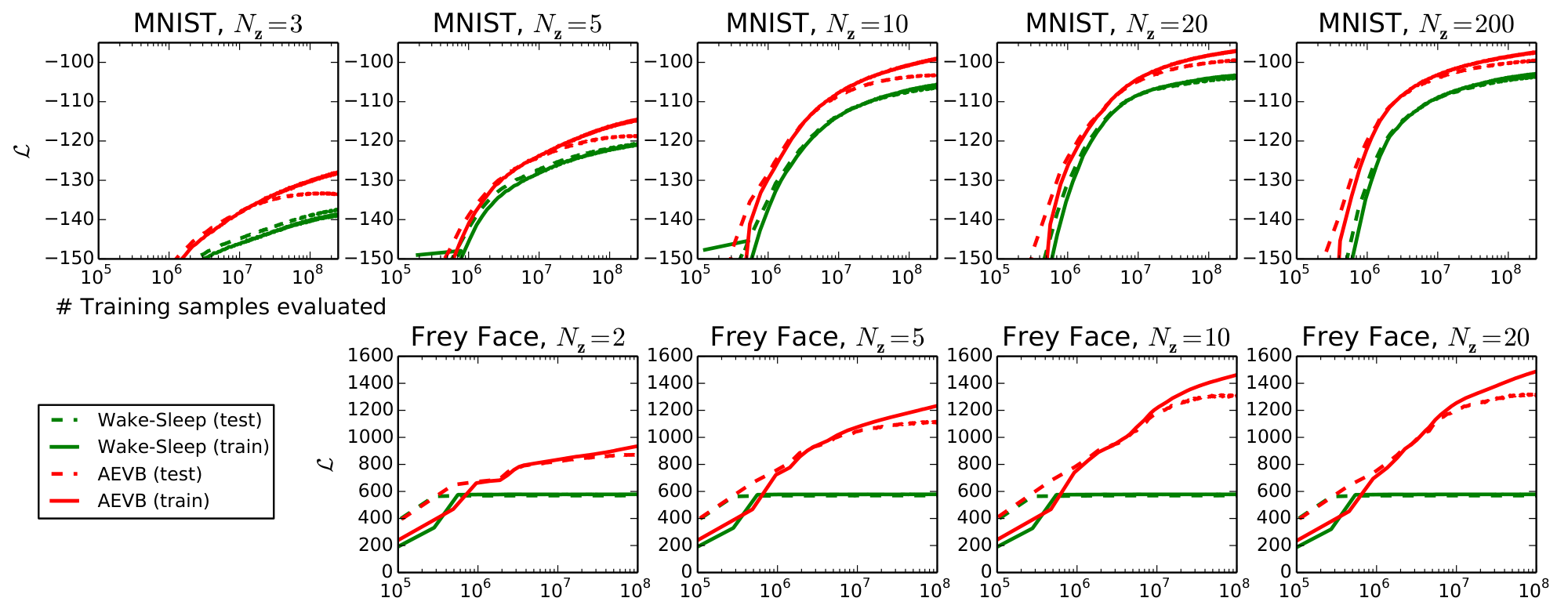
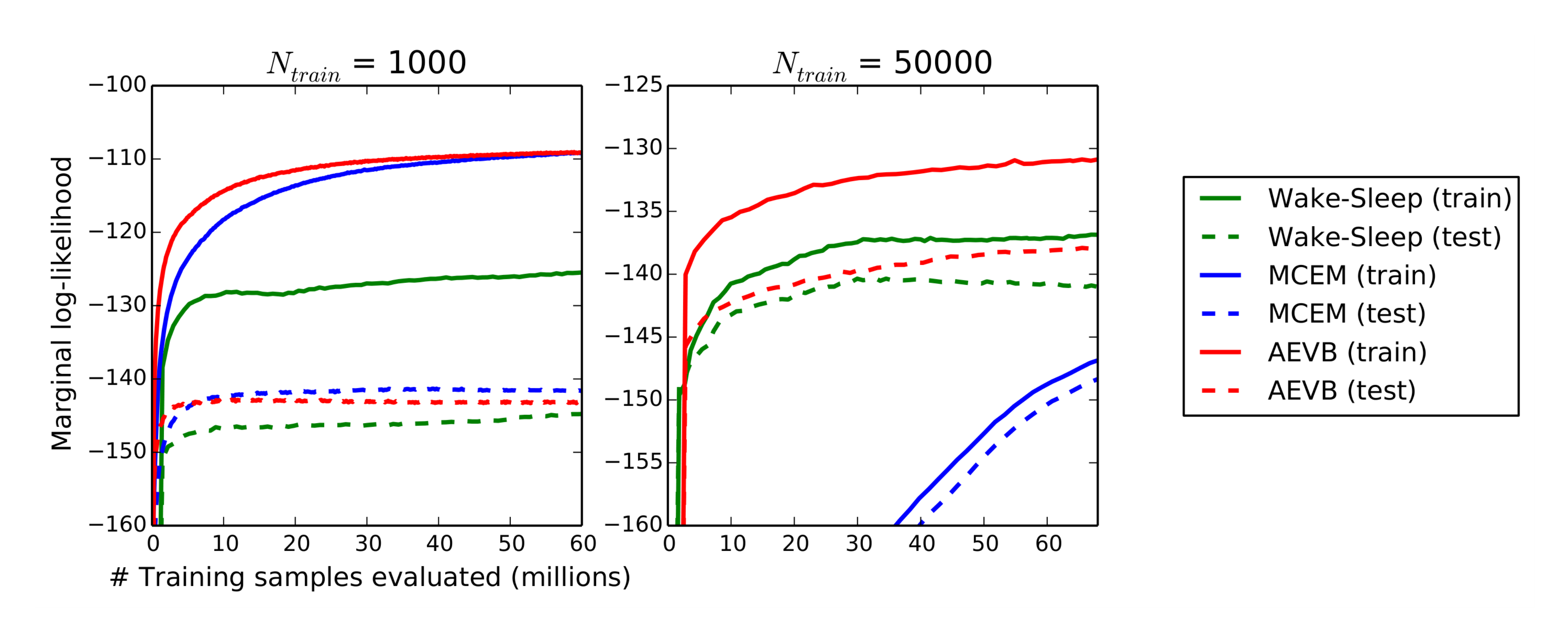
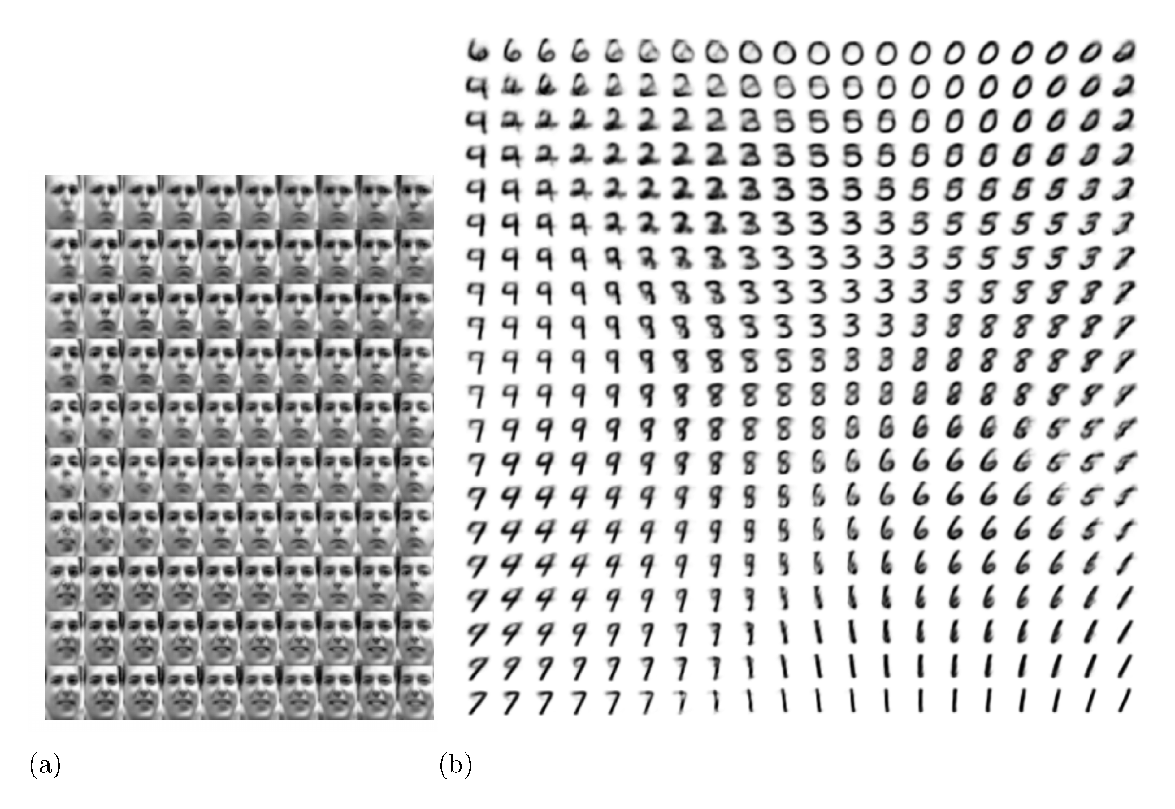
The core findings highlight AEVB's advantages. First, it converges 2–5 times faster than the wake-sleep algorithm and achieves 10–20% higher variational lower bounds on average across latent space dimensions from 2 to 200. Second, unlike prior methods, adding more latent variables (up to 200 dimensions) does not cause overfitting, thanks to built-in regularization from the KL divergence term, maintaining stable performance on test data. Third, AEVB yields marginal log-likelihoods about 5–10 nats higher than wake-sleep and outperforms Monte Carlo EM by converging in under 20 million samples for small sets (1,000 points) and scaling better for large ones (50,000 points), where EM becomes infeasible. Fourth, low-dimensional (2D) projections visualize meaningful manifolds, such as smooth interpolations between digit shapes in MNIST or facial expressions in Frey Faces. These results hold across experiments running in 20–40 minutes per million samples on standard hardware.
These findings imply that AEVB enables scalable, principled training of variational auto-encoders, bridging probabilistic modeling with auto-encoder architectures for better generative performance. It reduces risks of poor representations seen in unregularized auto-encoders by enforcing prior alignment, potentially cutting training times by half while improving data likelihood by 10–20%, which matters for downstream tasks like image synthesis, anomaly detection, or representation learning in safety-critical applications (e.g., medical imaging). Contrary to expectations from earlier work like wake-sleep, the method avoids dual-objective optimization pitfalls, delivering more reliable results without manual hyperparameter tuning for regularization.
To leverage these results, organizations should implement AEVB for training neural probabilistic models on image or sequential data, starting with Gaussian assumptions and neural encoders/decoders for quick pilots. The main option is using the lower-variance estimator (eq. 7 in the paper) for faster convergence, trading minimal added computation for stability; alternatives like full variational Bayes on parameters could be explored if parameter uncertainty is key. Further work is needed before broad deployment: validate on non-image data (e.g., text) and scale to deeper networks. Test via small-scale pilots on domain-specific datasets to confirm gains.
Limitations include reliance on continuous latent variables and differentiable reparameterizations (e.g., Gaussian families), which may not suit discrete data without extensions; high estimator variance could arise in non-standard distributions. Experiments are confined to toy datasets, so real-world scaling (e.g., millions of high-res images) requires more validation. Overall confidence is strong for the claimed efficiency and bounds, based on consistent empirical comparisons, but caution is advised for models outside tested assumptions like intractable non-Gaussian likelihoods.
1. Introduction
Section Summary: This section addresses the challenge of performing efficient approximate inference and learning in probabilistic models with continuous hidden variables or parameters that have hard-to-compute posterior distributions. It introduces the variational Bayesian method, which approximates the posterior but often struggles with the standard mean-field technique due to intractable calculations; to overcome this, the authors propose the Stochastic Gradient Variational Bayes (SGVB) estimator, a simple, differentiable tool that enables efficient optimization using common gradient-based methods for a wide range of such models. For datasets with independent data points and per-point continuous latents, they present the Auto-Encoding Variational Bayes (AEVB) algorithm, which trains a recognition model for fast inference via basic sampling, allowing efficient parameter learning without costly iterative methods, and supports tasks like denoising and visualization; when using a neural network for recognition, this leads to the variational auto-encoder.
How can we perform efficient approximate inference and learning with directed probabilistic models whose continuous latent variables and/or parameters have intractable posterior distributions? The variational Bayesian (VB) approach involves the optimization of an approximation to the intractable posterior. Unfortunately, the common mean-field approach requires analytical solutions of expectations w.r.t. the approximate posterior, which are also intractable in the general case. We show how a reparameterization of the variational lower bound yields a simple differentiable unbiased estimator of the lower bound; this SGVB (Stochastic Gradient Variational Bayes) estimator can be used for efficient approximate posterior inference in almost any model with continuous latent variables and/or parameters, and is straightforward to optimize using standard stochastic gradient ascent techniques.
For the case of an i.i.d. dataset and continuous latent variables per datapoint, we propose the Auto-Encoding VB (AEVB) algorithm. In the AEVB algorithm we make inference and learning especially efficient by using the SGVB estimator to optimize a recognition model that allows us to perform very efficient approximate posterior inference using simple ancestral sampling, which in turn allows us to efficiently learn the model parameters, without the need of expensive iterative inference schemes (such as MCMC) per datapoint. The learned approximate posterior inference model can also be used for a host of tasks such as recognition, denoising, representation and visualization purposes. When a neural network is used for the recognition model, we arrive at the variational auto-encoder.
2. Method
Section Summary: This section outlines a strategy for estimating parameters in directed graphical models that involve hidden continuous variables generating observed data, focusing on common scenarios with independent data samples where exact computations are infeasible. It addresses challenges like intractable integrals for likelihoods and posteriors, especially with large datasets that require efficient updates using small batches rather than slow sampling methods. The approach proposes approximate solutions for parameter estimation, inferring hidden variables from observations, and generating data distributions, using a jointly learned "recognition model" to approximate the hidden structure, akin to a probabilistic encoder for data representation.
The strategy in this section can be used to derive a lower bound estimator (a stochastic objective function) for a variety of directed graphical models with continuous latent variables. We will restrict ourselves here to the common case where we have an i.i.d. dataset with latent variables per datapoint, and where we like to perform maximum likelihood (ML) or maximum a posteriori (MAP) inference on the (global) parameters, and variational inference on the latent variables. It is, for example, straightforward to extend this scenario to the case where we also perform variational inference on the global parameters; that algorithm is put in the appendix, but experiments with that case are left to future work. Note that our method can be applied to online, non-stationary settings, e.g. streaming data, but here we assume a fixed dataset for simplicity.
2.1 Problem scenario
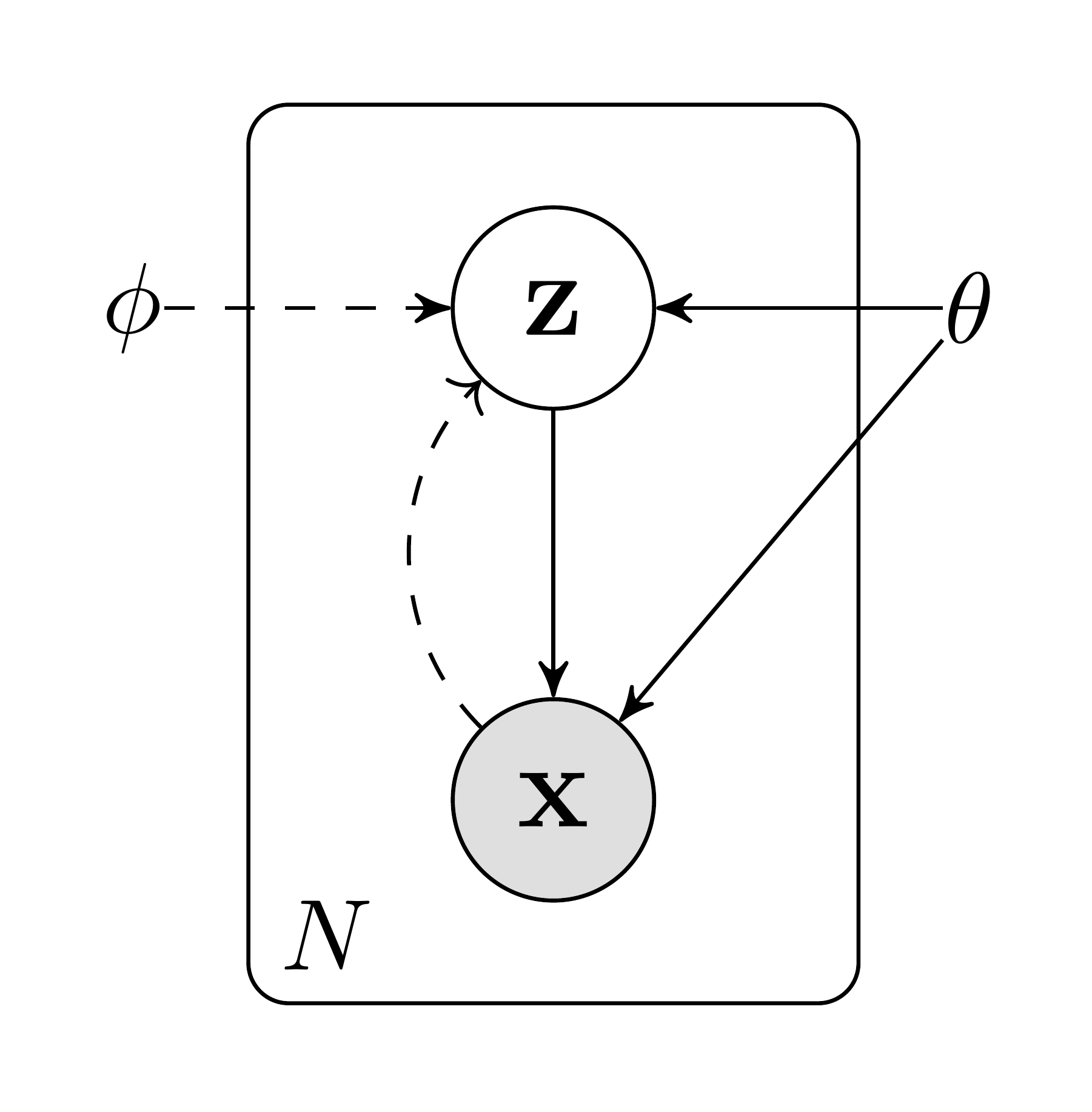
Let us consider some dataset $\mathbf{X} = {\mathbf{x}^{(i)}}{i=1}^N$ consisting of $N$ i.i.d. samples of some continuous or discrete variable $\mathbf{x}$. We assume that the data are generated by some random process, involving an unobserved continuous random variable $\mathbf{z}$. The process consists of two steps: (1) a value $\mathbf{z}^{(i)}$ is generated from some prior distribution $p{\boldsymbol{\theta}^*}(\mathbf{z})$; (2) a value $\mathbf{x}^{(i)}$ is generated from some conditional distribution $p_{\boldsymbol{\theta}^*}(\mathbf{x}| \mathbf{z})$. We assume that the prior $p_{\boldsymbol{\theta}^*}(\mathbf{z})$ and likelihood $p_{\boldsymbol{\theta}^*}(\mathbf{x}| \mathbf{z})$ come from parametric families of distributions $p_{\boldsymbol{\theta}}(\mathbf{z})$ and $p_{\boldsymbol{\theta}}(\mathbf{x}| \mathbf{z})$, and that their PDFs are differentiable almost everywhere w.r.t. both $\boldsymbol{\theta}$ and $\mathbf{z}$. Unfortunately, a lot of this process is hidden from our view: the true parameters $\boldsymbol{\theta}^*$ as well as the values of the latent variables $\mathbf{z}^{(i)}$ are unknown to us.
Very importantly, we do not make the common simplifying assumptions about the marginal or posterior probabilities. Conversely, we are here interested in a general algorithm that even works efficiently in the case of:
- Intractability: the case where the integral of the marginal likelihood $p_{\boldsymbol{\theta}}(\mathbf{x}) = \int p_{\boldsymbol{\theta}}(\mathbf{z}) p_{\boldsymbol{\theta}}(\mathbf{x}| \mathbf{z}) , d \mathbf{z}$ is intractable (so we cannot evaluate or differentiate the marginal likelihood), where the true posterior density $p_{\boldsymbol{\theta}}(\mathbf{z}| \mathbf{x}) = p_{\boldsymbol{\theta}}(\mathbf{x}| \mathbf{z})p_{\boldsymbol{\theta}}(\mathbf{z})/ p_{\boldsymbol{\theta}}(\mathbf{x})$ is intractable (so the EM algorithm cannot be used), and where the required integrals for any reasonable mean-field VB algorithm are also intractable. These intractabilities are quite common and appear in cases of moderately complicated likelihood functions $p_{\boldsymbol{\theta}}(\mathbf{x}| \mathbf{z})$, e.g. a neural network with a nonlinear hidden layer.
- A large dataset: we have so much data that batch optimization is too costly; we would like to make parameter updates using small minibatches or even single datapoints. Sampling-based solutions, e.g. Monte Carlo EM, would in general be too slow, since it involves a typically expensive sampling loop per datapoint.
We are interested in, and propose a solution to, three related problems in the above scenario:
- Efficient approximate ML or MAP estimation for the parameters $\boldsymbol{\theta}$. The parameters can be of interest themselves, e.g. if we are analyzing some natural process. They also allow us to mimic the hidden random process and generate artificial data that resembles the real data.
- Efficient approximate posterior inference of the latent variable $\mathbf{z}$ given an observed value $\mathbf{x}$ for a choice of parameters $\boldsymbol{\theta}$. This is useful for coding or data representation tasks.
- Efficient approximate marginal inference of the variable $\mathbf{x}$. This allows us to perform all kinds of inference tasks where a prior over $\mathbf{x}$ is required. Common applications in computer vision include image denoising, inpainting and super-resolution.
For the purpose of solving the above problems, let us introduce a recognition model $q_{\boldsymbol{\phi}}(\mathbf{z}| \mathbf{x})$: an approximation to the intractable true posterior $p_{\boldsymbol{\theta}}(\mathbf{z}| \mathbf{x})$. Note that in contrast with the approximate posterior in mean-field variational inference, it is not necessarily factorial and its parameters $\boldsymbol{\phi}$ are not computed from some closed-form expectation. Instead, we'll introduce a method for learning the recognition model parameters $\boldsymbol{\phi}$ jointly with the generative model parameters $\boldsymbol{\theta}$.
From a coding theory perspective, the unobserved variables $\mathbf{z}$ have an interpretation as a latent representation or code. In this paper we will therefore also refer to the recognition model $q_{\boldsymbol{\phi}}(\mathbf{z}| \mathbf{x})$ as a probabilistic encoder, since given a datapoint $\mathbf{x}$ it produces a distribution (e.g. a Gaussian) over the possible values of the code $\mathbf{z}$ from which the datapoint $\mathbf{x}$ could have been generated. In a similar vein we will refer to $p_{\boldsymbol{\theta}}(\mathbf{x}| \mathbf{z})$ as a probabilistic decoder, since given a code $\mathbf{z}$ it produces a distribution over the possible corresponding values of $\mathbf{x}$.
2.2 The variational bound
The marginal likelihood is composed of a sum over the marginal likelihoods of individual datapoints $\log p_{\boldsymbol{\theta}}(\mathbf{x}^{(1)}, \cdots, \mathbf{x}^{(N)}) = \sum_{i=1}^N \log p_{\boldsymbol{\theta}}(\mathbf{x}^{(i)})$, which can each be rewritten as:
$ \begin{align*} \log p_{\boldsymbol{\theta}}(\mathbf{x}^{(i)}) = D_{KL}(q_{\boldsymbol{\phi}}(\mathbf{z}| \mathbf{x}^{(i)})|| p_{\boldsymbol{\theta}}(\mathbf{z}| \mathbf{x}^{(i)})) + \mathcal{L}^{}(\boldsymbol{\theta}, \boldsymbol{\phi}; \mathbf{x}^{(i)}) \end{align*}\tag{1} $
The first RHS term is the KL divergence of the approximate from the true posterior. Since this KL-divergence is non-negative, the second RHS term $\mathcal{L}^{}(\boldsymbol{\theta}, \boldsymbol{\phi}; \mathbf{x}^{(i)})$ is called the (variational) lower bound on the marginal likelihood of datapoint $i$, and can be written as:
$ \begin{align*} \log p_{\boldsymbol{\theta}}(\mathbf{x}^{(i)}) \geq \mathcal{L}^{}(\boldsymbol{\theta}, \boldsymbol{\phi}; \mathbf{x}^{(i)}) &= \mathbb{E}{q{\boldsymbol{\phi}}(\mathbf{z}| \mathbf{x})}\left[- \log q_{\boldsymbol{\phi}}(\mathbf{z}| \mathbf{x}) + \log p_{\boldsymbol{\theta}}(\mathbf{x}, \mathbf{z})\right] \end{align*}\tag{2} $
which can also be written as:
$ \begin{align*} \mathcal{L}^{}(\boldsymbol{\theta}, \boldsymbol{\phi}; \mathbf{x}^{(i)}) = - D_{KL}(q_{\boldsymbol{\phi}}(\mathbf{z}| \mathbf{x}^{(i)}) || p_{\boldsymbol{\theta}}(\mathbf{z})) + \mathbb{E}{q{\boldsymbol{\phi}}(\mathbf{z}| \mathbf{x}^{(i)})}\left[\log p_{\boldsymbol{\theta}}(\mathbf{x}^{(i)} | \mathbf{z})\right] \end{align*}\tag{3} $
We want to differentiate and optimize the lower bound $\mathcal{L}^{}(\boldsymbol{\theta}, \boldsymbol{\phi}; \mathbf{x}^{(i)})$ w.r.t. both the variational parameters $\boldsymbol{\phi}$ and generative parameters $\boldsymbol{\theta}$. However, the gradient of the lower bound w.r.t. $\boldsymbol{\phi}$ is a bit problematic. The usual (naïve) Monte Carlo gradient estimator for this type of problem is: $\nabla_{\boldsymbol{\phi}} \mathbb{E}{q{\boldsymbol{\phi}}(\mathbf{z})}\left[f(\mathbf{z})\right] = \mathbb{E}{q{\boldsymbol{\phi}}(\mathbf{z})}\left[f(\mathbf{z}) \nabla_{q_{\boldsymbol{\phi}}(\mathbf{z})} \log q_{\boldsymbol{\phi}}(\mathbf{z}) \right] \simeq \frac{1}{L} \sum_{l=1}^L f(\mathbf{z}) \nabla_{q_{\boldsymbol{\phi}}(\mathbf{z}^{(l)})} \log q_{\boldsymbol{\phi}}(\mathbf{z}^{(l)})$ where $\mathbf{z}^{(l)} \sim q_{\boldsymbol{\phi}}(\mathbf{z}| \mathbf{x}^{(i)})$. This gradient estimator exhibits exhibits very high variance (see e.g. [1]) and is impractical for our purposes.
2.3 The SGVB estimator and AEVB algorithm
In this section we introduce a practical estimator of the lower bound and its derivatives w.r.t. the parameters. We assume an approximate posterior in the form $q_{\boldsymbol{\phi}}(\mathbf{z}| \mathbf{x})$, but please note that the technique can be applied to the case $q_{\boldsymbol{\phi}}(\mathbf{z})$, i.e. where we do not condition on $\mathbf{x}$, as well. The fully variational Bayesian method for inferring a posterior over the parameters is given in the appendix.
Under certain mild conditions outlined in Section 2.4 for a chosen approximate posterior $q_{\boldsymbol{\phi}}(\mathbf{z}| \mathbf{x})$ we can reparameterize the random variable $\widetilde{\mathbf{z}} \sim q_{\boldsymbol{\phi}}(\mathbf{z}| \mathbf{x})$ using a differentiable transformation $g_{\boldsymbol{\phi}}(\boldsymbol{\epsilon}, \mathbf{x})$ of an (auxiliary) noise variable $\boldsymbol{\epsilon}$:
$ \begin{align*} \widetilde{\mathbf{z}} = g_{\boldsymbol{\phi}}(\boldsymbol{\epsilon}, \mathbf{x}) \text{\quad with \quad} \boldsymbol{\epsilon} \sim p(\boldsymbol{\epsilon}) \end{align*}\tag{4} $
See Section 2.4 for general strategies for chosing such an approriate distribution $p(\boldsymbol{\epsilon})$ and function $g_{\boldsymbol{\phi}}(\boldsymbol{\epsilon}, \mathbf{x})$. We can now form Monte Carlo estimates of expectations of some function $f(\mathbf{z})$ w.r.t. $q_{\boldsymbol{\phi}}(\mathbf{z}| \mathbf{x})$ as follows:
$ \begin{align} \mathbb{E}{q{\boldsymbol{\phi}}(\mathbf{z}| \mathbf{x}^{(i)})}\left[f(\mathbf{z})\right] = \mathbb{E}{p(\boldsymbol{\epsilon})}\left[f(g{\boldsymbol{\phi}}(\boldsymbol{\epsilon}, \mathbf{x}^{(i)}))\right] &\simeq \frac{1}{L} \sum_{l=1}^L {f(g_{\boldsymbol{\phi}}(\boldsymbol{\epsilon}^{(l)}, \mathbf{x}^{(i)}))} \text{\quad where \quad} \boldsymbol{\epsilon}^{(l)} \sim p(\boldsymbol{\epsilon}) \end{align} $
We apply this technique to the variational lower bound (eq. 2), yielding our generic Stochastic Gradient Variational Bayes (SGVB) estimator $\widetilde{\mathcal{L}}^{A}(\boldsymbol{\theta}, \boldsymbol{\phi}; \mathbf{x}^{(i)}) \simeq \mathcal{L}^{}(\boldsymbol{\theta}, \boldsymbol{\phi}; \mathbf{x}^{(i)})$:
$ \begin{align*} \widetilde{\mathcal{L}}^{A}(\boldsymbol{\theta}, \boldsymbol{\phi}; \mathbf{x}^{(i)}) &= \frac{1}{L} \sum_{l=1}^L \log p_{\boldsymbol{\theta}}(\mathbf{x}^{(i)}, \mathbf{z}^{(i, l)}) - \log q_{\boldsymbol{\phi}}(\mathbf{z}^{(i, l)}| \mathbf{x}^{(i)}) \ \text{where \quad} \mathbf{z}^{(i, l)} &= g_{\boldsymbol{\phi}}(\boldsymbol{\epsilon}^{(i, l)}, \mathbf{x}^{(i)}) \text{\quad and \quad} \boldsymbol{\epsilon}^{(l)} \sim p(\boldsymbol{\epsilon}) \end{align*}\tag{5} $
Often, the KL-divergence $D_{KL}(q_{\boldsymbol{\phi}}(\mathbf{z}| \mathbf{x}^{(i)}) || p_{\boldsymbol{\theta}}(\mathbf{z}))$ of eq. 3 can be integrated analytically (see Appendix B), such that only the expected reconstruction error $\mathbb{E}{q{\boldsymbol{\phi}}(\mathbf{z}| \mathbf{x}^{(i)})}\left[\log p_{\boldsymbol{\theta}}(\mathbf{x}^{(i)} | \mathbf{z})\right]$ requires estimation by sampling. The KL-divergence term can then be interpreted as regularizing $\boldsymbol{\phi}$, encouraging the approximate posterior to be close to the prior $p_{\boldsymbol{\theta}}(\mathbf{z})$. This yields a second version of the SGVB estimator $\widetilde{\mathcal{L}}^{B}(\boldsymbol{\theta}, \boldsymbol{\phi}; \mathbf{x}^{(i)}) \simeq \mathcal{L}^{}(\boldsymbol{\theta}, \boldsymbol{\phi}; \mathbf{x}^{(i)})$, corresponding to eq. 3, which typically has less variance than the generic estimator:
$ \begin{align*} \widetilde{\mathcal{L}}^{B}(\boldsymbol{\theta}, \boldsymbol{\phi}; \mathbf{x}^{(i)}) &= - D_{KL}(q_{\boldsymbol{\phi}}(\mathbf{z}| \mathbf{x}^{(i)}) || p_{\boldsymbol{\theta}}(\mathbf{z}))
- \frac{1}{L} \sum_{l=1}^L (\log p_{\boldsymbol{\theta}}(\mathbf{x}^{(i)}| \mathbf{z}^{(i, l)})) \ \text{where \quad} \mathbf{z}^{(i, l)} &= g_{\boldsymbol{\phi}}(\boldsymbol{\epsilon}^{(i, l)}, \mathbf{x}^{(i)}) \text{\quad and \quad} \boldsymbol{\epsilon}^{(l)} \sim p(\boldsymbol{\epsilon}) \end{align*}\tag{6} $
Given multiple datapoints from a dataset $\mathbf{X}$ with $N$ datapoints, we can construct an estimator of the marginal likelihood lower bound of the full dataset, based on minibatches:
$ \begin{align*} \mathcal{L}^{}(\boldsymbol{\theta}, \boldsymbol{\phi}; \mathbf{X}) \simeq \widetilde{\mathcal{L}}^{M}(\boldsymbol{\theta}, \boldsymbol{\phi}; \mathbf{X}^M) = \frac{N}{M} \sum_{i=1}^M \widetilde{\mathcal{L}}^{}(\boldsymbol{\theta}, \boldsymbol{\phi}; \mathbf{x}^{(i)}) \end{align*}\tag{7} $
where the minibatch $\mathbf{X}^M = {\mathbf{x}^{(i)}}{i=1}^M$ is a randomly drawn sample of $M$ datapoints from the full dataset $\mathbf{X}$ with $N$ datapoints. In our experiments we found that the number of samples $L$ per datapoint can be set to $1$ as long as the minibatch size $M$ was large enough, e.g. $M=100$. Derivatives $\nabla{\boldsymbol{\theta}, \boldsymbol{\phi}} \widetilde{\mathcal{L}}(\boldsymbol{\theta}; \mathbf{X}^M)$ can be taken, and the resulting gradients can be used in conjunction with stochastic optimization methods such as SGD or Adagrad [2]. See Algorithm 1 for a basic approach to compute the stochastic gradients.
A connection with auto-encoders becomes clear when looking at the objective function given at eq. 6. The first term is (the KL divergence of the approximate posterior from the prior) acts as a regularizer, while the second term is a an expected negative reconstruction error. The function $g_{\boldsymbol{\phi}}(.)$ is chosen such that it maps a datapoint $\mathbf{x}^{(i)}$ and a random noise vector $\boldsymbol{\epsilon}^{(l)}$ to a sample from the approximate posterior for that datapoint: $\mathbf{z}^{(i, l)} = g_{\boldsymbol{\phi}}(\boldsymbol{\epsilon}^{(l)}, \mathbf{x}^{(i)})$ where $\mathbf{z}^{(i, l)} \sim q_{\boldsymbol{\phi}}(\mathbf{z}| \mathbf{x}^{(i)})$. Subsequently, the sample $\mathbf{z}^{(i, l)}$ is then input to function $\log p_{\boldsymbol{\theta}}(\mathbf{x}^{(i)}| \mathbf{z}^{(i, l)})$, which equals the probability density (or mass) of datapoint $\mathbf{x}^{(i)}$ under the generative model, given $\mathbf{z}^{(i, l)}$. This term is a negative reconstruction error in auto-encoder parlance.
$\boldsymbol{\theta}, \boldsymbol{\phi} \gets$ Initialize parameters
**repeat**
  $\mathbf{X}^M \gets $ Random minibatch of $M$ datapoints (drawn from full dataset)
  $\boldsymbol{\epsilon} \gets $ Random samples from noise distribution $p(\boldsymbol{\epsilon})$
  $\mathbf{g} \gets \nabla_{\boldsymbol{\theta}, \boldsymbol{\phi}} \widetilde{\mathcal{L}}^M(\boldsymbol{\theta}, \boldsymbol{\phi}; \mathbf{X}^M, \boldsymbol{\epsilon})$ (Gradients of minibatch estimator \eqref{eq:minibatchestimator})
  $\boldsymbol{\theta}, \boldsymbol{\phi} \gets $ Update parameters using gradients $\mathbf{g}$ (e.g. SGD or Adagrad ([2]))
**until** convergence of parameters $(\boldsymbol{\theta}, \boldsymbol{\phi})$
\\ **return** $\boldsymbol{\theta}, \boldsymbol{\phi}$
2.4 The reparameterization trick
In order to solve our problem we invoked an alternative method for generating samples from $q_{\boldsymbol{\phi}}(\mathbf{z}| \mathbf{x})$. The essential parameterization trick is quite simple. Let $\mathbf{z}$ be a continuous random variable, and $\mathbf{z} \sim q_{\boldsymbol{\phi}}(\mathbf{z}| \mathbf{x})$ be some conditional distribution. It is then often possible to express the random variable $\mathbf{z}$ as a deterministic variable $\mathbf{z} = g_{\boldsymbol{\phi}}(\boldsymbol{\epsilon}, \mathbf{x})$, where $\boldsymbol{\epsilon}$ is an auxiliary variable with independent marginal $p(\boldsymbol{\epsilon})$, and $g_{\boldsymbol{\phi}}(.)$ is some vector-valued function parameterized by $\boldsymbol{\phi}$.
This reparameterization is useful for our case since it can be used to rewrite an expectation w.r.t $q_{\boldsymbol{\phi}}(\mathbf{z}| \mathbf{x})$ such that the Monte Carlo estimate of the expectation is differentiable w.r.t. $\boldsymbol{\phi}$. A proof is as follows. Given the deterministic mapping $\mathbf{z} = g_{\boldsymbol{\phi}}(\boldsymbol{\epsilon}, \mathbf{x})$ we know that $q_{\boldsymbol{\phi}}(\mathbf{z}| \mathbf{x}) \prod_i d z_i = p(\boldsymbol{\epsilon}) \prod_i d \epsilon_i$. Therefore[^1], $\int q_{\boldsymbol{\phi}}(\mathbf{z}| \mathbf{x}) f(\mathbf{z}) , d \mathbf{z} = \int p(\boldsymbol{\epsilon}) f(\mathbf{z}) , d \boldsymbol{\epsilon} = \int p(\boldsymbol{\epsilon}) f(g_{\boldsymbol{\phi}}(\boldsymbol{\epsilon}, \mathbf{x})) , d \boldsymbol{\epsilon}$. It follows that a differentiable estimator can be constructed: $\int q_{\boldsymbol{\phi}}(\mathbf{z}| \mathbf{x}) f(\mathbf{z}) , d \mathbf{z} \simeq \frac{1}{L} \sum_{l=1}^L f(g_{\boldsymbol{\phi}}(\mathbf{x}, \boldsymbol{\epsilon}^{(l)}))$ where $\boldsymbol{\epsilon}^{(l)} \sim p(\boldsymbol{\epsilon})$. In Section 2.3 we applied this trick to obtain a differentiable estimator of the variational lower bound.
[^1]: Note that for infinitesimals we use the notational convention $d \mathbf{z} = \prod_i d z_i$
Take, for example, the univariate Gaussian case: let $z \sim p(z|x) = \mathcal{N}(\mu, \sigma^2)$. In this case, a valid reparameterization is $z = \mu + \sigma \epsilon$, where $\epsilon$ is an auxiliary noise variable $\epsilon \sim \mathcal{N}(0, 1)$. Therefore, $\mathbb{E}{\mathcal{N}(z; \mu, \sigma^2)}\left[f(z)\right] = \mathbb{E}{\mathcal{N}(\epsilon; 0, 1)}\left[f(\mu + \sigma \epsilon)\right] \simeq \frac{1}{L} \sum_{l=1}^L f(\mu + \sigma \epsilon^{(l)})$ where $\epsilon^{(l)} \sim \mathcal{N}(0, 1)$.
For which $q_{\boldsymbol{\phi}}(\mathbf{z}| \mathbf{x})$ can we choose such a differentiable transformation $g_{\boldsymbol{\phi}}(.)$ and auxiliary variable $\boldsymbol{\epsilon} \sim p(\boldsymbol{\epsilon})$? Three basic approaches are:
- Tractable inverse CDF. In this case, let $\boldsymbol{\epsilon} \sim \mathcal{U}(\mathbf{0}, \mathbf{I})$, and let $g_{\boldsymbol{\phi}}(\boldsymbol{\epsilon}, \mathbf{x})$ be the inverse CDF of $q_{\boldsymbol{\phi}}(\mathbf{z}| \mathbf{x})$. Examples: Exponential, Cauchy, Logistic, Rayleigh, Pareto, Weibull, Reciprocal, Gompertz, Gumbel and Erlang distributions.
- Analogous to the Gaussian example, for any "location-scale" family of distributions we can choose the standard distribution (with $\text{location} =0$, $\text{scale} =1$) as the auxiliary variable $\boldsymbol{\epsilon}$, and let $g(.)=\text{location}+\text{scale} \cdot \boldsymbol{\epsilon}$. Examples: Laplace, Elliptical, Student's t, Logistic, Uniform, Triangular and Gaussian distributions.
- Composition: It is often possible to express random variables as different transformations of auxiliary variables. Examples: Log-Normal (exponentiation of normally distributed variable), Gamma (a sum over exponentially distributed variables), Dirichlet (weighted sum of Gamma variates), Beta, Chi-Squared, and F distributions.
When all three approaches fail, good approximations to the inverse CDF exist requiring computations with time complexity comparable to the PDF (see e.g. [3] for some methods).
3. Example: Variational Auto-Encoder
Section Summary: This section describes a practical example of a variational auto-encoder, a type of neural network model that learns to generate data by compressing inputs into hidden variables and then reconstructing them. It uses a simple Gaussian distribution as the starting assumption for these hidden variables, with one neural network encoding input data into an approximate hidden representation and another decoding it back into the original form, handling either continuous or binary data. The model's parameters are trained together using a specialized algorithm that balances matching the hidden structure to a standard Gaussian while accurately rebuilding the data, making the complex underlying math workable through efficient calculations.
In this section we'll give an example where we use a neural network for the probabilistic encoder $q_{\boldsymbol{\phi}}(\mathbf{z}| \mathbf{x})$ (the approximation to the posterior of the generative model $p_{\boldsymbol{\theta}}(\mathbf{x}, \mathbf{z})$) and where the parameters $\boldsymbol{\phi}$ and $\boldsymbol{\theta}$ are optimized jointly with the AEVB algorithm.
Let the prior over the latent variables be the centered isotropic multivariate Gaussian $p_{\boldsymbol{\theta}}(\mathbf{z}) = \mathcal{N}(\mathbf{z}; \mathbf{0}, \mathbf{I})$. Note that in this case, the prior lacks parameters. We let $p_{\boldsymbol{\theta}}(\mathbf{x}| \mathbf{z})$ be a multivariate Gaussian (in case of real-valued data) or Bernoulli (in case of binary data) whose distribution parameters are computed from $\mathbf{z}$ with a MLP (a fully-connected neural network with a single hidden layer, see Appendix C). Note the true posterior $p_{\boldsymbol{\theta}}(\mathbf{z}| \mathbf{x})$ is in this case intractable. While there is much freedom in the form $q_{\boldsymbol{\phi}}(\mathbf{z}| \mathbf{x})$, we'll assume the true (but intractable) posterior takes on a approximate Gaussian form with an approximately diagonal covariance. In this case, we can let the variational approximate posterior be a multivariate Gaussian with a diagonal covariance structure[^2]:
[^2]: Note that this is just a (simplifying) choice, and not a limitation of our method.
$ \begin{align*} \log q_{\boldsymbol{\phi}}(\mathbf{z}| \mathbf{x}^{(i)}) &= \log \mathcal{N}(\mathbf{z}; \boldsymbol{\mu}^{(i)}, \boldsymbol{\sigma}^{2 (i)} \mathbf{I}) \end{align*}\tag{8} $
where the mean and s.d. of the approximate posterior, $\boldsymbol{\mu}^{(i)}$ and $\boldsymbol{\sigma}^{(i)}$, are outputs of the encoding MLP, i.e. nonlinear functions of datapoint $\mathbf{x}^{(i)}$ and the variational parameters $\boldsymbol{\phi}$ (see Appendix C).
As explained in Section 2.4, we sample from the posterior $\mathbf{z}^{(i, l)} \sim q_{\boldsymbol{\phi}}(\mathbf{z}| \mathbf{x}^{(i)})$ using $\mathbf{z}^{(i, l)} = g_{\boldsymbol{\phi}}(\mathbf{x}^{(i)}, \boldsymbol{\epsilon}^{(l)}) = \boldsymbol{\mu}^{(i)} + \boldsymbol{\sigma}^{(i)} \odot \boldsymbol{\epsilon}^{(l)}$ where $\boldsymbol{\epsilon}^{(l)} \sim \mathcal{N}(\mathbf{0}, \mathbf{I})$. With $\odot$ we signify an element-wise product. In this model both $p_{\boldsymbol{\theta}}(\mathbf{z})$ (the prior) and $q_{\boldsymbol{\phi}}(\mathbf{z}| \mathbf{x})$ are Gaussian; in this case, we can use the estimator of eq. 6 where the KL divergence can be computed and differentiated without estimation (see Appendix B). The resulting estimator for this model and datapoint $\mathbf{x}^{(i)}$ is:
$ \begin{align*} \mathcal{L}^{}(\boldsymbol{\theta}, \boldsymbol{\phi}; \mathbf{x}^{(i)}) &\simeq \frac{1}{2} \sum_{j=1}^J \left(1 + \log ((\sigma_j^{(i)})^2) - (\mu_j^{(i)})^2 - (\sigma_j^{(i)})^2 \right)
- \frac{1}{L} \sum_{l=1}^L \log p_{\boldsymbol{\theta}}(\mathbf{x}^{(i)}| \mathbf{z}^{(i, l)}) \ \text{where\quad} \mathbf{z}^{(i, l)} &= \boldsymbol{\mu}^{(i)} + \boldsymbol{\sigma}^{(i)} \odot \boldsymbol{\epsilon}^{(l)} \text{\quad and \quad} \boldsymbol{\epsilon}^{(l)} \sim \mathcal{N}(0, \mathbf{I}) \end{align*}\tag{9} $
As explained above and in Appendix C, the decoding term $\log p_{\boldsymbol{\theta}}(\mathbf{x}^{(i)}| \mathbf{z}^{(i, l)})$ is a Bernoulli or Gaussian MLP, depending on the type of data we are modelling.
4. Related work
Section Summary: This section reviews existing techniques for training models with hidden variables, highlighting the wake-sleep algorithm as the main alternative for online learning in continuous latent variable models, though it optimizes separate objectives without directly improving the model's overall likelihood and works for discrete variables too. It also covers advances in stochastic variational inference to lower estimation errors using tricks like reparameterization, and draws parallels between the authors' method and auto-encoders, which reconstruct data but often need extra tweaks for useful features, while their approach builds in natural regularization. Finally, it touches on related ideas in sparse coding, generative networks, and recent independent work linking auto-encoders to similar probabilistic learning for directed models, mostly limited to specific cases like binary variables.
The wake-sleep algorithm [4] is, to the best of our knowledge, the only other on-line learning method in the literature that is applicable to the same general class of continuous latent variable models. Like our method, the wake-sleep algorithm employs a recognition model that approximates the true posterior. A drawback of the wake-sleep algorithm is that it requires a concurrent optimization of two objective functions, which together do not correspond to optimization of (a bound of) the marginal likelihood. An advantage of wake-sleep is that it also applies to models with discrete latent variables. Wake-Sleep has the same computational complexity as AEVB per datapoint.
Stochastic variational inference [5] has recently received increasing interest. Recently, [1] introduced a control variate schemes to reduce the high variance of the naïve gradient estimator discussed in Section 2.1, and applied to exponential family approximations of the posterior. In [6] some general methods, i.e. a control variate scheme, were introduced for reducing the variance of the original gradient estimator. In [7], a similar reparameterization as in this paper was used in an efficient version of a stochastic variational inference algorithm for learning the natural parameters of exponential-family approximating distributions.
The AEVB algorithm exposes a connection between directed probabilistic models (trained with a variational objective) and auto-encoders. A connection between linear auto-encoders and a certain class of generative linear-Gaussian models has long been known. In [8] it was shown that PCA corresponds to the maximum-likelihood (ML) solution of a special case of the linear-Gaussian model with a prior $p(\mathbf{z}) = \mathcal{N}(0, \mathbf{I})$ and a conditional distribution $p(\mathbf{x}| \mathbf{z}) = \mathcal{N}(\mathbf{x}; \mathbf{W} \mathbf{z}, \epsilon \mathbf{I})$, specifically the case with infinitesimally small $\epsilon$.
In relevant recent work on autoencoders [9] it was shown that the training criterion of unregularized autoencoders corresponds to maximization of a lower bound (see the infomax principle [10]) of the mutual information between input $X$ and latent representation $Z$. Maximizing (w.r.t. parameters) of the mutual information is equivalent to maximizing the conditional entropy, which is lower bounded by the expected loglikelihood of the data under the autoencoding model [9], i.e. the negative reconstrution error. However, it is well known that this reconstruction criterion is in itself not sufficient for learning useful representations [11]. Regularization techniques have been proposed to make autoencoders learn useful representations, such as denoising, contractive and sparse autoencoder variants [11]. The SGVB objective contains a regularization term dictated by the variational bound (e.g. eq. 9), lacking the usual nuisance regularization hyperparameter required to learn useful representations. Related are also encoder-decoder architectures such as the predictive sparse decomposition (PSD) [12], from which we drew some inspiration. Also relevant are the recently introduced Generative Stochastic Networks [13] where noisy auto-encoders learn the transition operator of a Markov chain that samples from the data distribution. In [14] a recognition model was employed for efficient learning with Deep Boltzmann Machines. These methods are targeted at either unnormalized models (i.e. undirected models like Boltzmann machines) or limited to sparse coding models, in contrast to our proposed algorithm for learning a general class of directed probabilistic models.
The recently proposed DARN method [15], also learns a directed probabilistic model using an auto-encoding structure, however their method applies to binary latent variables. Even more recently, [16] also make the connection between auto-encoders, directed proabilistic models and stochastic variational inference using the reparameterization trick we describe in this paper. Their work was developed independently of ours and provides an additional perspective on AEVB.