Pixel Recurrent Neural Networks

Aaron van den OordNal KalchbrennerKoray Kavukcuoglu

article2016ICML2,903 citationsBest Paper Award

Introduces two-dimensional recurrent neural network architectures with residual connections to sequentially model discrete pixel dependencies, setting a new standard for generative image modeling and log-likelihood performance on ImageNet.

Listen

Pixel Recurrent Neural Networks advance generative modeling of natural images by treating pixel prediction as a sequential task that captures full spatial and color dependencies. The work addresses the core difficulty of building models that are simultaneously expressive enough to represent complex image structure, tractable enough to compute exact likelihoods, and scalable to large datasets—an obstacle that has limited prior approaches such as latent-variable models and earlier autoregressive networks.

The authors set out to demonstrate that two-dimensional recurrent architectures can achieve substantially higher likelihoods on standard image benchmarks while also producing coherent samples. They constructed three main variants: Row LSTM and Diagonal BiLSTM networks that use specialized convolutional recurrences to scan images row-wise or diagonally, and a fully convolutional PixelCNN that trades unbounded context for greater parallelism during training. All models factor the joint distribution over raw RGB pixels into a product of conditional multinomial distributions implemented with softmax layers, enforce correct conditioning through masked convolutions, and employ residual connections to train networks up to twelve layers deep. Experiments covered MNIST, CIFAR-10, and ImageNet images resized to 32×32 and 64×64 pixels, with performance measured by negative log-likelihood after appropriate noise dequantization.

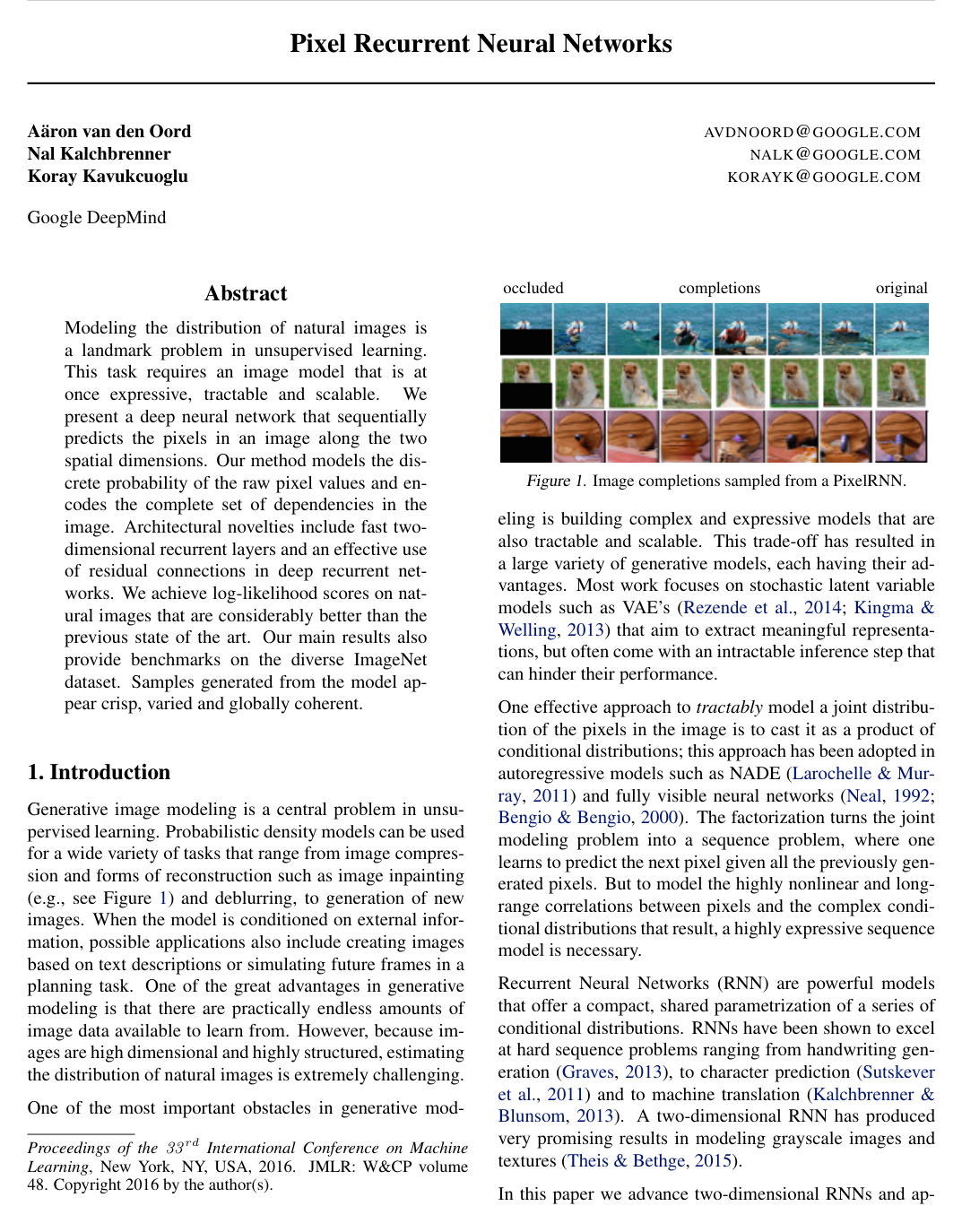
The strongest model, a twelve-layer Diagonal BiLSTM, reached 79.20 nats on MNIST and 3.00 bits per dimension on CIFAR-10, improving on previous published results by roughly 1–2 nats and 0.47 bits per dimension respectively. On ImageNet the same family of models established the first reported likelihood baselines at 3.86 bits per dimension for 32×32 images and 3.63 bits per dimension for 64×64 images. Samples drawn from the networks appear sharp and globally consistent, and image-completion examples show that the models fill occluded regions with diverse yet plausible content. Architectural ablations confirmed that the discrete softmax output outperforms continuous mixture-density alternatives and that residual connections enable effective scaling with depth.

These gains indicate that autoregressive recurrent models can now serve as practical density estimators for high-resolution images, supporting downstream uses such as lossless compression, inpainting, and conditional generation. Because likelihood improves steadily with added depth and data, further increases in model size and training compute are expected to yield additional gains. Generation remains inherently sequential, however, so practical deployment at high resolution will require either faster sampling techniques or hybrid architectures that combine the accuracy of PixelRNNs with the speed of parallel alternatives.

Google probability recurrent networks supervised machine learning Pixel Recurrent Neural Networks PixelCNN architecture Multi-Scale PixelRNN

arXiv: 1601.06759

No sufficiently relevant recommendations were found.

Paper: Video Pixel Networks, Nal Kalchbrenner et al. (2017). This work carries PixelRNN’s masked pixel-level prediction into video, extending its dependency modeling across both space and time.
Paper: Image Transformer, Niki Parmar et al. (2018). Building on autoregressive image modeling, this paper replaces recurrent and convolutional context mechanisms with self-attention to capture broader visual dependencies more efficiently.
Paper: Generating Diverse High-Fidelity Images with VQ-VAE-2, Ali Razavi et al. (2019). This work advances PixelCNN-style autoregressive modeling by applying it to compressed, hierarchical image codes rather than generating every pixel directly.
Paper: Very Deep VAEs Generalize Autoregressive Models and Can Outperform Them on Images, Rewon Child (2021). After seeing PixelRNN establish strong image likelihoods, this paper tests whether much deeper hierarchical VAEs can match or surpass autoregressive models while avoiding their slow sequential generation.

Cover for Pixel Recurrent Neural Networks

Abstract

Modeling the distribution of natural images is a landmark problem in unsupervised learning. This task requires an image model that is at once expressive, tractable and scalable. We present a deep neural network that sequentially predicts the pixels in an image along the two spatial dimensions. Our method models the discrete probability of the raw pixel values and encodes the complete set of dependencies in the image. Architectural novelties include fast two-dimensional recurrent layers and an effective use of residual connections in deep recurrent networks. We achieve log-likelihood scores on natural images that are considerably better than the previous state of the art. Our main results also provide benchmarks on the diverse ImageNet dataset. Samples generated from the model appear crisp, varied and globally coherent.

Topics

probability recurrent networks supervised machine learning unsupervised learning network architecture

Keywords

Pixel Recurrent Neural Networks PixelCNN architecture Multi-Scale PixelRNN Row LSTM image modeling neural autoregressive distribution estimator image completion

1 Introduction
2 Model
2.1 Generating an Image Pixel by Pixel
2.2 Pixels as Discrete Variables
3 Pixel Recurrent Neural Networks
3.1 Row LSTM
3.2 Diagonal BiLSTM
3.3 Residual Connections
3.4 Masked Convolution
3.5 PixelCNN
3.6 Multi-Scale PixelRNN
4 Specifications of Models
5 Experiments
5.1 Evaluation
5.2 Training Details
5.3 Discrete Softmax Distribution
5.4 Residual Connections
5.5 MNIST
5.6 CIFAR-10
5.7 ImageNet
6 Conclusion
References

Knowls

Knowl 1 — Autoregressive Factorization of Image Distributions Across Pixels and Channels
model/method
The joint probability distribution $p(\mathbf{x})$ of an image $\mathbf{x}$ of spatial dimension $n \times n$ pixels is modeled as an autoregressive product of conditional probabilities over a 1D sequence of pixels $x_1, \dots, x_{n^2}$ scanned row by row and pixel by pixel from top-left to bottom-right:

$p(\mathbf{x}) = \prod_{i=1}^{n^2} p(x_i \mid x_1, \dots, x_{i-1})$

where $x_i$ is the $i$ -th pixel in raster scan order, and $\mathbf{x}_{<i} = (x_1, \dots, x_{i-1})$ denotes the history of all previously scanned pixels.

To model the full inter-channel dependencies within each RGB pixel $x_i = (x_{i,R}, x_{i,G}, x_{i,B})$ , the conditional distribution $p(x_i \mid \mathbf{x}_{<i})$ is factorized across color channels:

$p(x_i \mid \mathbf{x}_{<i}) = p(x_{i,R} \mid \mathbf{x}_{<i}) \, p(x_{i,G} \mid \mathbf{x}_{<i}, x_{i,R}) \, p(x_{i,B} \mid \mathbf{x}_{<i}, x_{i,R}, x_{i,G})$

Under this factorization, the Red channel is conditioned on all prior pixels; the Green channel is conditioned on all prior pixels and the current Red channel; and the Blue channel is conditioned on all prior pixels along with both current Red and Green channels. During training and evaluation, conditional distributions across all pixels and channels are evaluated in parallel, whereas image sampling is executed sequentially.
Knowl 2 — Discrete Categorical Softmax for Pixel Intensity Modeling
model/method
Rather than modeling raw pixel intensities as continuous variables using continuous density functions or mixture models, each 8-bit color channel intensity $x_{i,*} \in \{0, 1, \dots, 255\}$ is treated as a discrete random variable with a 256-way categorical distribution parameterized by a softmax layer:

$p(x_{i,*} = v \mid \text{context}) = \frac{\exp(z_v)}{\sum_{k=0}^{255} \exp(z_k)}$

where $z_0, \dots, z_{255}$ are unnormalized logit activations generated by the network for that subpixel.

Key properties of this discrete formulation include:
- Arbitrary representational capacity: it represents multimodal, asymmetric, highly peaked (e.g., at 0 or 255), or long-tailed conditional distributions without imposing prior parametric shape constraints.
- Bounded support: it prevents probability mass leakage outside the valid range $[0, 255]$ .
- Comparability to continuous density models: when continuous density models evaluate on dequantized data with added uniform noise $u \in [0, 1)$ , their log-likelihood is directly comparable to the discrete distribution log-likelihood, because the discrete distribution corresponds to a continuous piecewise-uniform density function with constant value $p(x_{i,*})$ over each unit interval $[v, v+1)$ .
Knowl 3 — Masked Convolutions for Causal Conditioning
model/method
To preserve autoregressive causal conditioning across 2D spatial positions and RGB color channels in standard and recurrent convolutional layers, convolutional weight tensors are elementwise multiplied by binary masks that zero out non-causal connections. The feature maps at each layer are partitioned along the feature channel dimension into three equal groups representing Red, Green, and Blue channels.

Two mask configurations are defined:
- Mask A: Applied exclusively to the first convolutional layer of the network. It zeroes out all filter weights corresponding to future spatial pixel locations (rows below the center pixel, and columns to the right of the center pixel in the center row). At the center pixel $(0, 0)$ , it zeroes out connections from Red to Red, Green to Green, Blue to Blue, Green to Red, Blue to Red, and Blue to Green. Consequently, the Red output depends only on past pixels; the Green output depends on past pixels and the current Red input; and the Blue output depends on past pixels and current Red and Green inputs.
- Mask B: Applied to all subsequent convolutional layers and input-to-state recurrent transformations. It enforces the same spatial masking as Mask A, but relaxes the center-pixel channel constraint by allowing connections from each color channel to itself (Red connects to Red; Green connects to Green and Red; Blue connects to Blue, Green, and Red).
Knowl 4 — Row LSTM Layer
model/method
The Row LSTM is a unidirectional recurrent layer that processes an image row by row from top to bottom, computing the hidden states for an entire row at once using 1D convolutions.

For an input feature map $\mathbf{x}$ of spatial size $n \times n$ with $h$ feature channels:
- Input-to-State Component: Precomputed for the whole image in parallel using a masked $k \times 1$ convolution along each row ( $k \ge 3$ ), yielding a tensor of shape $4h \times n \times n$ containing pre-activations for the four LSTM gates.
- Recurrent State-to-State Component: For each row $i \in \{1, \dots, n\}$ , given the previous row hidden state $\mathbf{h}_{i-1} \in \mathbb{R}^{h \times n \times 1}$ and cell state $\mathbf{c}_{i-1} \in \mathbb{R}^{h \times n \times 1}$ , the gate activations and updated states $\mathbf{h}_i, \mathbf{c}_i \in \mathbb{R}^{h \times n \times 1}$ are computed via:
$\begin{bmatrix} \mathbf{o}_i \\ \mathbf{f}_i \\ \mathbf{i}_i \\ \mathbf{g}_i \end{bmatrix} = \begin{bmatrix} \sigma \\ \sigma \\ \sigma \\ \tanh \end{bmatrix} \left( \mathbf{K}^{ss} \circledast \mathbf{h}_{i-1} + \mathbf{K}^{is} \circledast \mathbf{x}_i \right)$

$\mathbf{c}_i = \mathbf{f}_i \odot \mathbf{c}_{i-1} + \mathbf{i}_i \odot \mathbf{g}_i$

$\mathbf{h}_i = \mathbf{o}_i \odot \tanh(\mathbf{c}_i)$

where $\circledast$ denotes a 1D convolution of kernel size $k \times 1$ , $\odot$ represents elementwise multiplication, $\sigma$ is the elementwise logistic sigmoid function, $\mathbf{K}^{ss}$ is the state-to-state convolution kernel, and $\mathbf{K}^{is} \circledast \mathbf{x}_i$ is the precomputed input-to-state term for row $i$ .

Because the state updates are propagated row-wise with a 1D convolution of width $k$ , the receptive field of the Row LSTM is bounded by a triangular wedge extending upwards from the target pixel, leaving pixels in the upper corners outside the context window.
Knowl 5 — Diagonal BiLSTM Layer
model/method
The Diagonal BiLSTM is a recurrent neural network layer designed to capture the complete causal context (all pixels above and to the left of the current pixel) while parallelizing state computation along diagonals of the image.

The algorithm computes states as follows:
1. Input Skewing: An $n \times n$ feature map is skewed by shifting each row $r \in \{0, \dots, n-1\}$ to the right by $r$ positions, producing a skewed map of size $n \times (2n - 1)$ .
2. Diagonal Recurrence:
  - The input-to-state contribution is computed over the skewed map with a $1 \times 1$ convolution $\mathbf{K}^{is}$ , producing a $4h \times n \times (2n - 1)$ tensor.
  - The recurrent state-to-state transition processes the skewed representation column by column (which corresponds to diagonal by diagonal in the original image coordinates) using a $2 \times 1$ column convolution $\mathbf{K}^{ss}$ :
$\begin{bmatrix} \mathbf{o}_d \\ \mathbf{f}_d \\ \mathbf{i}_d \\ \mathbf{g}_d \end{bmatrix} = \begin{bmatrix} \sigma \\ \sigma \\ \sigma \\ \tanh \end{bmatrix} \left( \mathbf{K}^{ss} \circledast \mathbf{h}_{d-1} + \mathbf{K}^{is} \circledast \mathbf{x}_d \right)$

$\mathbf{c}_d = \mathbf{f}_d \odot \mathbf{c}_{d-1} + \mathbf{i}_d \odot \mathbf{g}_d$

$\mathbf{h}_d = \mathbf{o}_d \odot \tanh(\mathbf{c}_d)$
1. Unskewing: The hidden state tensor of shape $n \times (2n - 1)$ is shifted back by reversing row offsets to produce an $n \times n$ feature map.
2. Bidirectional Aggregation: Steps 1-3 are computed in two directions: top-left to bottom-right and top-right to bottom-left. To avoid violating causal conditioning, the right-to-left output map is shifted down by one row and added elementwise to the left-to-right output map.
A $2 \times 1$ state convolution along the diagonal provides an unbounded receptive field covering the entire causal context above and to the left of each pixel.
Knowl 6 — PixelCNN Architecture
model/method
The PixelCNN is a fully convolutional autoregressive architecture for image generation that models conditional pixel distributions without recurrent state loops.

Structural properties include:
- Spatial Preservation: Maintains input spatial resolution $n \times n$ across all hidden layers without pooling or spatial downsampling operations.
- Masked Convolutions: Composed of stacked convolutional layers (e.g., 15 layers) utilizing $3 \times 3$ masked kernels. The initial layer employs Mask A to enforce strict channel and pixel causality; subsequent hidden layers use Mask B to allow channel self-connections.
- Receptive Field: Possesses a bounded causal receptive field that scales linearly with depth ( $1 + 2L$ pixels for $L$ layers of $3 \times 3$ convolutions).
- Parallelism: During training and log-likelihood evaluation, all pixels and feature maps are computed entirely in parallel in a single forward pass. During sample generation, execution is strictly sequential, requiring $n^2$ forward evaluations as each generated pixel is iteratively fed back as input.
Knowl 7 — Residual Bottleneck Connections in Deep PixelRNNs
model/method
To train deep PixelRNNs up to 12 LSTM layers without optimization degradation, residual bottleneck blocks wrap each recurrent layer:
1. The input feature map to a block has $2h$ feature channels.
2. The input-to-state projection reduces dimensionality from $2h$ to $h$ per gate ( $4h$ channels in total across the 4 LSTM gates) via a masked convolution.
3. The recurrent LSTM layer (Row LSTM or Diagonal BiLSTM) computes hidden state representations of channel dimension $h$ .
4. A $1 \times 1$ convolution upsamples the recurrent output from $h$ back to $2h$ feature channels.
5. The input feature map is added directly to the projected output:
$\mathbf{y} = \mathbf{x}_{\text{in}} + \text{Conv}_{1 \times 1}(\text{LSTM}(\mathbf{x}_{\text{in}}))$

This residual mechanism provides direct signal and gradient pathways across recurrent layers without requiring additional recurrent gate parameters.
Knowl 8 — Multi-Scale PixelRNN Architecture
model/method
The Multi-Scale PixelRNN is a hierarchical generative model designed to capture both long-range global coherence and local details in higher-resolution images (such as $64 \times 64$ pixels).

The framework consists of:
1. Unconditional Base PixelRNN: Autoregressively generates a subsampled low-resolution image of size $s \times s$ (e.g., $32 \times 32$ ).
2. Upsampling Conditioning Network: Consists of convolutional and deconvolutional layers that project the $s \times s$ image into an upsampled feature map of shape $c \times n \times n$ , where $n \times n$ is the target full image resolution and $c$ is the number of feature channels.
3. Conditional PixelRNN: Generates the final $n \times n$ image pixel by pixel. At every layer of this network, the $c \times n \times n$ conditioning map is transformed by an unmasked $1 \times 1$ convolution into a $4h \times n \times n$ bias tensor, which is added directly to the layer's input-to-state pre-activation maps prior to recurrent updates.

Knowl 9 — Ablation Analysis of Output Distribution, Residual Connections, and Network Depth

empirical result

Ablations on the CIFAR-10 validation set evaluate the impact of discrete vs. continuous output distributions, residual connections, skip connections, and network depth on negative log-likelihood (NLL, in bits/dim):

Discrete Softmax vs. Continuous Mixture: A 12-layer Row LSTM with a 256-way discrete Softmax achieves 3.06 bits/dim, outperforming the same model trained with a continuous Mixture of Conditional Gaussian Scale Mixtures (MCGSM), which achieves 3.22 bits/dim.
Residual and Skip Connections (12-layer Row LSTM):

Residual connections and layer-to-output skip connections independently improve negative log-likelihood, and combining both achieves the lowest NLL of 3.06 bits/dim.

Network Depth (Row LSTM with residual and skip connections):

NLL monotonically decreases as depth increases from 1 to 12 LSTM layers.

Knowl 10 — Generative Modeling Benchmarks on MNIST, CIFAR-10, and ImageNet

data/table

The PixelRNN and PixelCNN architectures established new state-of-the-art negative log-likelihood (NLL) density estimation scores across standard benchmarks.

Binarized MNIST Test Performance (NLL in nats):

Model	NLL Test (nats)
DBM 2hl	$\approx 84.62$
DBN 2hl	$\approx 84.55$
NADE	88.33
EoNADE 2hl (128 orderings)	85.10
EoNADE-5 2hl (128 orderings)	84.68
DLGM	$\approx 86.60$
DLGM 8 leapfrog steps	$\approx 85.51$
DARN 1hl	$\approx 84.13$
MADE 2hl (32 masks)	86.64
DRAW	$\le 80.97$
PixelCNN	81.30
Row LSTM	80.54
Diagonal BiLSTM (1 layer, $h=32$ )	80.75
Diagonal BiLSTM (7 layers, $h=16$ )	79.20

CIFAR-10 Test Performance (NLL in bits/dim, training score in parentheses):

Model	NLL Test (Train) [bits/dim]
Uniform Distribution	8.00
Multivariate Gaussian	4.70
NICE	4.48
Deep Diffusion	4.20
Deep GMMs	4.00
RIDE	3.47
PixelCNN (15 layers, $h=128$ )	3.14 (3.08)
Row LSTM (12 layers, $h=128$ )	3.07 (3.00)
Diagonal BiLSTM (12 layers, $h=128$ )	3.00 (2.93)

Performance directly tracks receptive field capacity: Diagonal BiLSTM (unbounded global context) outperforms Row LSTM (triangular context), which in turn outperforms PixelCNN (bounded convolutional context).

Downsampled ImageNet Validation Performance (NLL in bits/dim, training score in parentheses):

Coverage note — No substantial contributed material was omitted; minor GPU training hyperparameters and standard optimizer settings are summarized within the experimental knowls.

References

1.Bengio, Yoshua and Bengio, Samy. Modeling high-dimensional discrete data with multi-layer neural networks. pp. 400–406. MIT Press, 2000.
2.Dinh, Laurent, Krueger, David, and Bengio, Yoshua. NICE: Non-linear independent components estimation. arXiv preprint arXiv:1410.8516, 2014.
3.Germain, Mathieu, Gregor, Karol, Murray, Iain, and Larochelle, Hugo. MADE: Masked autoencoder for distribution estimation. arXiv preprint arXiv:1502.03509, 2015.
4.Graves, Alex. Generating sequences with recurrent neural networks. arXiv preprint arXiv:1308.0850, 2013.
5.Graves, Alex and Schmidhuber, Jürgen. Offline handwriting recognition with multidimensional recurrent neural networks. In Advances in Neural Information Processing Systems, 2009.
6.Gregor, Karol, Danihelka, Ivo, Mnih, Andriy, Blundell, Charles, and Wierstra, Daan. Deep autoregressive networks. In Proceedings of the 31st International Conference on Machine Learning, 2014.
7.Gregor, Karol, Danihelka, Ivo, Graves, Alex, and Wierstra, Daan. DRAW: A recurrent neural network for image generation. Proceedings of the 32nd International Conference on Machine Learning, 2015.
8.He, Kaiming, Zhang, Xiangyu, Ren, Shaoqing, and Sun, Jian. Deep residual learning for image recognition. arXiv preprint arXiv:1512.03385, 2015.
9.Hochreiter, Sepp and Schmidhuber, Jürgen. Long short-term memory. Neural computation, 1997.
10.Kalchbrenner, Nal and Blunsom, Phil. Recurrent continuous translation models. In Proceedings of the 2013 Conference on Empirical Methods in Natural Language Processing, 2013.
11.Kalchbrenner, Nal, Danihelka, Ivo, and Graves, Alex. Grid long short-term memory. arXiv preprint arXiv:1507.01526, 2015.
12.Kingma, Diederik P and Welling, Max. Auto-encoding variational bayes. arXiv preprint arXiv:1312.6114, 2013.
13.Krizhevsky, Alex. Learning multiple layers of features from tiny images. 2009.
14.Larochelle, Hugo and Murray, Iain. The neural autoregressive distribution estimator. The Journal of Machine Learning Research, 2011.
15.LeCun, Yann, Bottou, Léon, Bengio, Yoshua, and Haffner, Patrick. Gradient-based learning applied to document recognition. Proceedings of the IEEE, 1998.
16.Murray, Iain and Salakhutdinov, Ruslan R. Evaluating probabilities under high-dimensional latent variable models. In Advances in Neural Information Processing Systems, 2009.
17.Neal, Radford M. Connectionist learning of belief networks. Artificial intelligence, 1992.
18.Raiko, Tapani, Li, Yao, Cho, Kyunghyun, and Bengio, Yoshua. Iterative neural autoregressive distribution estimator NADE-k. In Advances in Neural Information Processing Systems, 2014.
19.Rezende, Danilo J, Mohamed, Shakir, and Wierstra, Daan. Stochastic backpropagation and approximate inference in deep generative models. In Proceedings of the 31st International Conference on Machine Learning, 2014.
20.Russakovsky, Olga, Deng, Jia, Su, Hao, Krause, Jonathan, Satheesh, Sanjeev, Ma, Sean, Huang, Zhiheng, Karpathy, Andrej, Khosla, Aditya, Bernstein, Michael, Berg, Alexander C., and Fei-Fei, Li. ImageNet Large Scale Visual Recognition Challenge. International Journal of Computer Vision (IJCV), 2015.
21.Salakhutdinov, Ruslan and Hinton, Geoffrey E. Deep boltzmann machines. In International Conference on Artificial Intelligence and Statistics, 2009.
22.Salakhutdinov, Ruslan and Murray, Iain. On the quantitative analysis of deep belief networks. In Proceedings of the 25th international conference on Machine learning, 2008.
23.Salimans, Tim, Kingma, Diederik P, and Welling, Max. Markov chain monte carlo and variational inference: Bridging the gap. Proceedings of the 32nd International Conference on Machine Learning, 2015.
24.Sohl-Dickstein, Jascha, Weiss, Eric A., Maheswaranathan, Niru, and Ganguli, Surya. Deep unsupervised learning using nonequilibrium thermodynamics. Proceedings of the 32nd International Conference on Machine Learning, 2015.
25.Stollenga, Marijn F, Byeon, Wonmin, Liwicki, Marcus, and Schmidhuber, Juergen. Parallel multi-dimensional lstm, with application to fast biomedical volumetric image segmentation. In Advances in Neural Information Processing Systems 28. 2015.
26.Sutskever, Ilya, Martens, James, and Hinton, Geoffrey E. Generating text with recurrent neural networks. In Proceedings of the 28th International Conference on Machine Learning, 2011.
27.Theis, Lucas and Bethge, Matthias. Generative image modeling using spatial LSTMs. In Advances in Neural Information Processing Systems, 2015.
28.Theis, Lucas, van den Oord, Aäron, and Bethge, Matthias. A note on the evaluation of generative models. arXiv preprint arXiv:1511.01844, 2015.
29.Uria, Benigno, Murray, Iain, and Larochelle, Hugo. RNADE: The real-valued neural autoregressive density-estimator. In Advances in Neural Information Processing Systems, 2013.
30.Uria, Benigno, Murray, Iain, and Larochelle, Hugo. A deep and tractable density estimator. In Proceedings of the 31st International Conference on Machine Learning, 2014.
31.van den Oord, Aäron and Schrauwen, Benjamin. Factoring variations in natural images with deep gaussian mixture models. In Advances in Neural Information Processing Systems, 2014a.
32.van den Oord, Aäron and Schrauwen, Benjamin. The student-t mixture as a natural image patch prior with application to image compression. The Journal of Machine Learning Research, 2014b.
33.Zhang, Yu, Chen, Guoguo, Yu, Dong, Yao, Kaisheng, Khudanpur, Sanjeev, and Glass, James. Highway long short-term memory RNNs for distant speech recognition. In Proceedings of the International Conference on Acoustics, Speech and Signal Processing, 2016.

Citation

MLA

Oord, A. van . den ., et al. “Pixel Recurrent Neural Networks”. arXiv, 2016, https://doi.org/10.48550/arxiv.1601.06759.

APA

Oord, A. van . den ., Kalchbrenner, N., & Kavukcuoglu, K. (2016). Pixel Recurrent Neural Networks. arXiv. https://doi.org/10.48550/arxiv.1601.06759

Chicago

Oord, A. van . den ., N. Kalchbrenner, and K. Kavukcuoglu. 2016. “Pixel Recurrent Neural Networks”. Preprint, ArXiv. https://doi.org/10.48550/arxiv.1601.06759.

Harvard

Oord, A. van . den ., Kalchbrenner, N. and Kavukcuoglu, K. (2016) “Pixel Recurrent Neural Networks”. arXiv. Available at: https://doi.org/10.48550/arxiv.1601.06759.

Vancouver

1. Oord A van den, Kalchbrenner N, Kavukcuoglu K (2016) Pixel Recurrent Neural Networks. https://doi.org/10.48550/arxiv.1601.06759

BibTeX

@misc{https://doi.org/10.48550/arxiv.1601.06759,
  doi = {10.48550/ARXIV.1601.06759},
  url = {https://arxiv.org/abs/1601.06759},
  author = {Oord, Aaron van den and Kalchbrenner, Nal and Kavukcuoglu, Koray},
  keywords = {Computer Vision and Pattern Recognition (cs.CV), Machine Learning (cs.LG), Neural and Evolutionary Computing (cs.NE), FOS: Computer and information sciences, FOS: Computer and information sciences},
  title = {Pixel Recurrent Neural Networks},
  publisher = {arXiv},
  year = {2016},
  copyright = {arXiv.org perpetual, non-exclusive license}
}

Metadata:DOI registry

Access the Paper

This paper is available from its original source. Click below to access the PDF.

Open PDF

License: Published with permission

Number of layers	1	2	3	6	9	12
NLL (bits/dim)	3.30	3.20	3.17	3.09	3.08	3.06

Image Size	NLL Validation (Train) [bits/dim]
$32 \times 32$ (12-layer Row LSTM, $h=384$ )	3.86 (3.83)
$64 \times 64$ (4-layer Row LSTM, $h=512$ )	3.63 (3.57)

Pixel Recurrent Neural Networks

Abstract

Topics

Keywords

Table of Contents

Knowls

Knowl 1 — Autoregressive Factorization of Image Distributions Across Pixels and Channels

Knowl 2 — Discrete Categorical Softmax for Pixel Intensity Modeling

Knowl 3 — Masked Convolutions for Causal Conditioning

Knowl 4 — Row LSTM Layer

Knowl 5 — Diagonal BiLSTM Layer

Knowl 6 — PixelCNN Architecture