Classifier-Free Diffusion Guidance

Jonathan Ho & Tim Salimans
Google Research, Brain team
{jonathanho,salimans}@google.com

Abstract

Classifier guidance is a recently introduced method to trade off mode coverage and sample fidelity in conditional diffusion models post training, in the same spirit as low temperature sampling or truncation in other types of generative models. Classifier guidance combines the score estimate of a diffusion model with the gradient of an image classifier and thereby requires training an image classifier separate from the diffusion model. It also raises the question of whether guidance can be performed without a classifier. We show that guidance can be indeed performed by a pure generative model without such a classifier: in what we call classifier-free guidance, we jointly train a conditional and an unconditional diffusion model, and we combine the resulting conditional and unconditional score estimates to attain a trade-off between sample quality and diversity similar to that obtained using classifier guidance.[^1]

[^1]: A short version of this paper appeared in the NeurIPS 2021 Workshop on Deep Generative Models and Downstream Applications: https://openreview.net/pdf?id=qw8AKxfYbI

Executive Summary: Diffusion models represent a powerful class of generative AI systems that create realistic images, audio, and other data by gradually adding and then removing noise. A key challenge in these models is balancing sample diversity—producing varied outputs—with fidelity, or how closely samples match real data in quality. Traditional methods like classifier guidance improve fidelity but require training a separate image classifier on noisy data, complicating the process and raising questions about whether such guidance truly relies on generative power alone or adversarial tricks against the classifier. This issue matters now as diffusion models surpass older techniques like GANs in applications such as image synthesis for design, entertainment, and research, demanding simpler, more reliable ways to optimize output without added complexity.

This paper introduces and evaluates classifier-free guidance, a technique that achieves similar fidelity-diversity trade-offs in conditional diffusion models—those generating images based on labels like "dog" or "car"—without any external classifier. It demonstrates that a single model can learn both conditional and unconditional generation, enabling guided sampling through simple mixing of internal estimates.

The approach trains a unified neural network on the ImageNet dataset, a large collection of labeled photos used as a benchmark for image generation. During training, the model processes noisy versions of images across various noise levels, sometimes ignoring the class label (with 10-20% probability) to learn unconditional generation. No separate classifier is trained; instead, sampling combines the model's predictions for conditional and unconditional paths, weighted by a guidance strength parameter (w) from 0 (no guidance) to 4 or higher. Experiments used standard model setups on downsampled ImageNet at 64x64 and 128x128 resolutions, generating 50,000 samples per test to measure Fréchet Inception Distance (FID, lower is better for diversity and realism) and Inception Score (IS, higher is better for quality and variety within classes). Training spanned hundreds of thousands of steps over weeks on high-end hardware, with sampling in 128 to 1,024 steps.

The core findings show classifier-free guidance effectively controls output trade-offs. First, increasing w from 0 to 4 monotonically worsens FID (from about 1.6 to 24 on 64x64 ImageNet) while boosting IS (from 66 to 260), mirroring truncation in GANs but without blurriness from naive tweaks. Second, low guidance (w=0.1-0.3) yields top FID scores—1.55 on 64x64 and 2.43 on 128x128—outperforming prior classifier-guided models like ADM-G (FID 2.97) and even GANs like BigGAN-deep. Third, high guidance (w=4) achieves record IS of 422 on 128x128, surpassing BigGAN-deep's 253 while maintaining competitive FID around 21. Fourth, a low unconditional training rate (10-20%) suffices for strong results, using minimal capacity. Fifth, more sampling steps (256 versus 128) improve metrics by 20-30% in IS and FID but double computation time due to dual model evaluations per step.

These results imply that diffusion models can deliver state-of-the-art image quality using purely generative mechanisms, avoiding the pipeline overhead and potential adversarial artifacts of classifiers. This simplifies deployment, cuts training costs by eliminating extra models, and confirms diffusion's edge over GANs in flexibility without mimicking their weaknesses. Unlike expectations that classifiers are essential for peak performance, classifier-free guidance matches or exceeds them with less capacity, suggesting broader applicability to underrepresented data or non-image tasks. It enhances safety in AI-generated content by reducing reliance on classifiers that could be gamed, though high guidance risks lower diversity, potentially amplifying biases in imbalanced datasets.

Adopt classifier-free guidance as the default for conditional diffusion models, tuning w based on priorities: low w (0.1-0.3) for diverse, realistic outputs in exploratory uses; high w (3-4) for high-fidelity single-class generation like concept art. For production, prioritize models with 10% unconditional training and 256 sampling steps to balance speed and quality. Next, test on diverse datasets beyond ImageNet, such as medical images or audio, and optimize architectures for single-pass sampling to halve inference time—perhaps by late-stage conditioning injection. If diversity loss is a concern, pilot hybrid methods preserving variance. Strong decisions require validating on real-world tasks, as benchmarks like FID/IS may not capture all perceptual nuances.

Key limitations include doubled sampling cost from dual predictions, making it slower than classifier guidance despite simpler training; results used hyperparameters tuned for prior methods, so custom optimization could yield further gains. Data gaps exist for non-class-conditional settings, and assumptions like uniform noise schedules may not generalize. Confidence is high for ImageNet-style image generation, backed by reproducible metrics outperforming baselines, but caution applies to edge cases like rare classes where unconditional training might underperform.

1. Introduction

Section Summary: Diffusion models are a powerful type of generative AI that create high-quality images and audio with fewer steps than some rivals, but early versions struggled to produce sharp, focused samples without extra help. Classifier guidance improved this by using a separate trained model to steer the process, much like adjusting settings in other AI generators, though it required training an additional classifier on noisy data and raised concerns about it just tricking classifiers rather than truly enhancing generation. To avoid these issues, the authors introduce classifier-free guidance, which blends outputs from conditional and unconditional versions of the same diffusion model, achieving similar quality boosts and proving that diffusion models alone can rival top generative techniques.

Diffusion models have recently emerged as an expressive and flexible family of generative models, delivering competitive sample quality and likelihood scores on image and audio synthesis tasks ([1, 2, 3, 4, 5, 6]). These models have delivered audio synthesis performance rivaling the quality of autoregressive models with substantially fewer inference steps ([7, 8]), and they have delivered ImageNet generation results outperforming BigGAN-deep ([9]) and VQ-VAE-2 ([10]) in terms of FID score and classification accuracy score ([11, 12]).

[12] proposed classifier guidance, a technique to boost the sample quality of a diffusion model using an extra trained classifier. Prior to classifier guidance, it was not known how to generate "low temperature" samples from a diffusion model similar to those produced by truncated BigGAN ([9]) or low temperature Glow ([13]): naive attempts, such as scaling the model score vectors or decreasing the amount of Gaussian noise added during diffusion sampling, are ineffective ([12]). Classifier guidance instead mixes a diffusion model's score estimate with the input gradient of the log probability of a classifier. By varying the strength of the classifier gradient, [12] can trade off Inception score ([14]) and FID score ([15]) (or precision and recall) in a manner similar to varying the truncation parameter of BigGAN.

We are interested in whether classifier guidance can be performed without a classifier. Classifier guidance complicates the diffusion model training pipeline because it requires training an extra classifier, and this classifier must be trained on noisy data so it is generally not possible to plug in a pre-trained classifier. Furthermore, because classifier guidance mixes a score estimate with a classifier gradient during sampling, classifier-guided diffusion sampling can be interpreted as attempting to confuse an image classifier with a gradient-based adversarial attack. This raises the question of whether classifier guidance is successful at boosting classifier-based metrics such as FID and Inception score (IS) simply because it is adversarial against such classifiers. Stepping in direction of classifier gradients also bears some resemblance to GAN training, particularly with nonparameteric generators; this also raises the question of whether classifier-guided diffusion models perform well on classifier-based metrics because they are beginning to resemble GANs, which are already known to perform well on such metrics.

To resolve these questions, we present classifier-free guidance, our guidance method which avoids any classifier entirely. Rather than sampling in the direction of the gradient of an image classifier, classifier-free guidance instead mixes the score estimates of a conditional diffusion model and a jointly trained unconditional diffusion model. By sweeping over the mixing weight, we attain a FID/IS tradeoff similar to that attained by classifier guidance. Our classifier-free guidance results demonstrate that pure generative diffusion models are capable of synthesizing extremely high fidelity samples possible with other types of generative models.

2. Background

Section Summary: This section describes the foundational setup for training diffusion models in continuous time, where a forward process gradually adds noise to original data through a Markov chain, transforming clean samples into pure noise while tracking a log signal-to-noise ratio. The reverse process, powered by a neural network, starts from random noise and iteratively denoises it to reconstruct or generate new data, using a trained predictor that estimates the noise added at each step. The model is optimized via a loss that encourages accurate noise prediction across varying noise levels, enabling efficient sampling in discrete steps that approximate the continuous generation path.

We train diffusion models in continuous time ([4, 7, 5]): letting $\mathbf{x} \sim p(\mathbf{x})$ and $\mathbf{z} = {\mathbf{z}\lambda , |, \lambda \in [\lambda{\mathrm{min}}, \lambda_{\mathrm{max}}]}$ for hyperparameters $\lambda_{\mathrm{min}} < \lambda_{\mathrm{max}} \in \mathbb{R}$, the forward process $q(\mathbf{z}| \mathbf{x})$ is the variance-preserving Markov process ([1]):

$ \begin{align} q(\mathbf{z}\lambda| \mathbf{x}) &= \mathcal{N}(\alpha\lambda \mathbf{x}, \sigma_\lambda^2 \mathbf{I}), \ \text{where}\ \alpha_\lambda^2 = 1/(1+e^{-\lambda}), \ \sigma_\lambda^2 = 1-\alpha_\lambda^2 \ q(\mathbf{z}{\lambda} | \mathbf{z}{\lambda'}) &= \mathcal{N}((\alpha_{\lambda}/\alpha_{\lambda'})\mathbf{z}{\lambda'}, \sigma{\lambda|\lambda'}^2 \mathbf{I}), \ \text{where}\ \lambda < \lambda',
\sigma^2_{\lambda|\lambda'} = (1-e^{\lambda-\lambda'})\sigma_\lambda^2 \end{align} $

We will use the notation $p(\mathbf{z})$ (or $p(\mathbf{z}\lambda)$) to denote the marginal of $\mathbf{z}$ (or $\mathbf{z}\lambda$) when $\mathbf{x} \sim p(\mathbf{x})$ and $\mathbf{z} \sim q(\mathbf{z}|\mathbf{x})$. Note that $\lambda = \log \alpha_\lambda^2 / \sigma_\lambda^2$, so $\lambda$ can be interpreted as the log signal-to-noise ratio of $\mathbf{z}_\lambda$, and the forward process runs in the direction of decreasing $\lambda$.

Conditioned on $\mathbf{x}$, the forward process can be described in reverse by the transitions $q(\mathbf{z}{\lambda'}| \mathbf{z}\lambda, \mathbf{x}) = \mathcal{N}(\tilde {\boldsymbol{\mu}}{\lambda'|\lambda}(\mathbf{z}\lambda, \mathbf{x}), \tilde\sigma^2_{\lambda'|\lambda}\mathbf{I})$, where

$ \begin{align} \tilde {\boldsymbol{\mu}}{\lambda'|\lambda}(\mathbf{z}\lambda, \mathbf{x}) = e^{\lambda-\lambda'}(\alpha_{\lambda'}/\alpha_{\lambda})\mathbf{z}\lambda + (1-e^{\lambda - \lambda'})\alpha{\lambda'}\mathbf{x}, \quad \tilde\sigma^2_{\lambda'|\lambda} = (1-e^{\lambda-\lambda'})\sigma_{\lambda}^2 \end{align} $

The reverse process generative model starts from $p_\theta(\mathbf{z}{\lambda{\mathrm{min}}}) = \mathcal{N}(\mathbf{0}, \mathbf{I})$. We specify the transitions:

$ \begin{align} p_\theta(\mathbf{z}{\lambda'}| \mathbf{z}{\lambda}) = \mathcal{N}(\tilde {\boldsymbol{\mu}}{\lambda'|\lambda}(\mathbf{z}\lambda, \mathbf{x}\theta(\mathbf{z}\lambda)), (\tilde\sigma^2_{\lambda'|\lambda})^{1-v} (\sigma^2_{\lambda|\lambda'})^v) \end{align} $

During sampling, we apply this transition along an increasing sequence $\lambda_{\mathrm{min}} = \lambda_1 < \dots < \lambda_T = \lambda_{\mathrm{max}}$ for $T$ timesteps; in other words, we follow the discrete time ancestral sampler of [1, 3]. If the model $\mathbf{x}\theta$ is correct, then as $T \to \infty$, we obtain samples from an SDE whose sample paths are distributed as $p(\mathbf{z})$ ([4]), and we use $p\theta(\mathbf{z})$ to denote the continuous time model distribution. The variance is a log-space interpolation of $\tilde\sigma^2_{\lambda'|\lambda}$ and $\sigma^2_{\lambda|\lambda'}$ as suggested by [16]; we found it effective to use a constant hyperparameter $v$ rather than learned $\mathbf{z}\lambda$-dependent $v$. Note that the variances simplify to $\tilde\sigma^2{\lambda'|\lambda}$ as $\lambda'\rightarrow\lambda$, so $v$ has an effect only when sampling with non-infinitesimal timesteps as done in practice.

The reverse process mean comes from an estimate $\mathbf{x}\theta(\mathbf{z}\lambda) \approx \mathbf{x}$ plugged into $q(\mathbf{z}{\lambda'}| \mathbf{z}\lambda, \mathbf{x})$ ([3, 5]) ($\mathbf{x}\theta$ also receives $\lambda$ as input, but we suppress this to keep our notation clean). We parameterize $\mathbf{x}\theta$ in terms of ${\boldsymbol{\epsilon}}$-prediction ([3]): $\mathbf{x}\theta(\mathbf{z}\lambda) = (\mathbf{z}\lambda - \sigma\lambda {\boldsymbol{\epsilon}}\theta(\mathbf{z}\lambda)) / \alpha_\lambda$, and we train on the objective

$ \begin{align} \mathbb{E}{{\boldsymbol{\epsilon}}, \lambda}!\left[| {\boldsymbol{\epsilon}}\theta(\mathbf{z}_\lambda) - {\boldsymbol{\epsilon}} |^2_2\right] \end{align} $

where ${\boldsymbol{\epsilon}} \sim \mathcal{N}(\mathbf{0}, \mathbf{I})$, $\mathbf{z}\lambda = \alpha\lambda \mathbf{x} + \sigma_\lambda {\boldsymbol{\epsilon}}$, and $\lambda$ is drawn from a distribution $p(\lambda)$ over $[\lambda_{\mathrm{min}}, \lambda_{\mathrm{max}}]$. This objective is denoising score matching ([17, 18]) over multiple noise scales ([2]), and when $p(\lambda)$ is uniform, the objective is proportional to the variational lower bound on the marginal log likelihood of the latent variable model $\int p_\theta(\mathbf{x}| \mathbf{z}) p_\theta(\mathbf{z}) d \mathbf{z}$, ignoring the term for the unspecified decoder $p_\theta(\mathbf{x}| \mathbf{z})$ and for the prior at $\mathbf{z}{\lambda\mathrm{min}}$ ([5]).

If $p(\lambda)$ is not uniform, the objective can be interpreted as weighted variational lower bound whose weighting can be tuned for sample quality ([3, 5]). We use a $p(\lambda)$ inspired by the discrete time cosine noise schedule of [16]: we sample $\lambda$ via $\lambda = -2\log\tan(au+b)$ for uniformly distributed $u \in [0, 1]$, where $b = \arctan(e^{-\lambda_{\mathrm{max}}/2})$ and $a = \arctan(e^{-\lambda_{\mathrm{min}}/2}) - b$. This represents a hyperbolic secant distribution modified to be supported on a bounded interval. For finite timestep generation, we use $\lambda$ values corresponding to uniformly spaced $u \in [0, 1]$, and the final generated sample is $\mathbf{x}\theta(\mathbf{z}{\lambda_\mathrm{max}})$.

Because the loss for ${\boldsymbol{\epsilon}}\theta(\mathbf{z}\lambda)$ is denoising score matching for all $\lambda$, the score ${\boldsymbol{\epsilon}}\theta(\mathbf{z}\lambda)$ learned by our model estimates the gradient of the log-density of the distribution of our noisy data $\mathbf{z}\lambda$, that is ${\boldsymbol{\epsilon}}\theta(\mathbf{z}\lambda) \approx -\sigma\lambda \nabla_{\mathbf{z}\lambda}\log p(\mathbf{z}\lambda)$; note, however, that because we use unconstrained neural networks to define ${\boldsymbol{\epsilon}}\theta$, there need not exist any scalar potential whose gradient is ${\boldsymbol{\epsilon}}\theta$. Sampling from the learned diffusion model resembles using Langevin diffusion to sample from a sequence of distributions $p(\mathbf{z}_\lambda)$ that converges to the conditional distribution $p(\mathbf{x})$ of the original data $\mathbf{x}$.

In the case of conditional generative modeling, the data $\mathbf{x}$ is drawn jointly with conditioning information $\mathbf{c}$, i.e. a class label for class-conditional image generation. The only modification to the model is that the reverse process function approximator receives $\mathbf{c}$ as input, as in ${\boldsymbol{\epsilon}}\theta(\mathbf{z}\lambda, \mathbf{c})$.

3. Guidance

Section Summary: Generative models like GANs and flow-based models can use techniques such as truncation or low-temperature sampling to produce higher-quality samples with less variety by adjusting noise inputs, but these methods don't work well in diffusion models, often resulting in blurry outputs. To address this, classifier guidance modifies the diffusion process by incorporating gradients from a separate classifier that favors samples easy to label correctly, boosting perceptual quality metrics like the Inception score at the cost of sample diversity. Classifier-free guidance achieves a similar tradeoff without needing an external classifier, by training the diffusion model on both conditional and unconditional data to self-guide the generation process.

An interesting property of certain generative models, such as GANs and flow-based models, is the ability to perform truncated or low temperature sampling by decreasing the variance or range of noise inputs to the generative model at sampling time. The intended effect is to decrease the diversity of the samples while increasing the quality of each individual sample. Truncation in BigGAN ([9]), for example, yields a tradeoff curve between FID score and Inception score for low and high amounts of truncation, respectively. Low temperature sampling in Glow ([13]) has a similar effect.

Unfortunately, straightforward attempts of implementing truncation or low temperature sampling in diffusion models are ineffective. For example, scaling model scores or decreasing the variance of Gaussian noise in the reverse process cause the diffusion model to generate blurry, low quality samples ([12]).

3.1 Classifier guidance

To obtain a truncation-like effect in diffusion models, [12] introduce classifier guidance, where the diffusion score ${\boldsymbol{\epsilon}}\theta(\mathbf{z}\lambda, \mathbf{c}) \approx -\sigma_\lambda \nabla_{\mathbf{z}\lambda}\log p(\mathbf{z}\lambda | \mathbf{c})$ is modified to include the gradient of the log likelihood of an auxiliary classifier model $p_{\theta}(\mathbf{c} | \mathbf{z}_\lambda)$ as follows:

$ \tilde{{\boldsymbol{\epsilon}}}\theta(\mathbf{z}\lambda, \mathbf{c}) = {\boldsymbol{\epsilon}}\theta(\mathbf{z}\lambda, \mathbf{c}) - w\sigma_{\lambda}\nabla_{\mathbf{z}\lambda}\log p{\theta}(\mathbf{c} | \mathbf{z}\lambda) \approx -\sigma{\lambda}\nabla_{\mathbf{z}\lambda}[\log p(\mathbf{z}\lambda | \mathbf{c}) + w \log p_{\theta}(\mathbf{c} | \mathbf{z}_\lambda)], $

where $w$ is a parameter that controls the strength of the classifier guidance. This modified score $\tilde{{\boldsymbol{\epsilon}}}\theta(\mathbf{z}\lambda, \mathbf{c})$ is then used in place of ${\boldsymbol{\epsilon}}\theta(\mathbf{z}\lambda, \mathbf{c})$ when sampling from the diffusion model, resulting in approximate samples from the distribution

$ \tilde{p}{\theta}(\mathbf{z}\lambda | \mathbf{c}) \propto p_{\theta}(\mathbf{z}\lambda | \mathbf{c})p{\theta}(\mathbf{c} | \mathbf{z}_\lambda)^{w}. $

The effect is that of up-weighting the probability of data for which the classifier $p_{\theta}(\mathbf{c} | \mathbf{z}_\lambda)$ assigns high likelihood to the correct label: data that can be classified well scores high on the Inception score of perceptual quality ([14]), which rewards generative models for this by design. [12] therefore find that by setting $w > 0$ they can improve the Inception score of their diffusion model, at the expense of decreased diversity in their samples.

Figure 2 illustrates the effect of numerically solved guidance $\tilde{p}{\theta}(\mathbf{z}\lambda | \mathbf{c}) \propto p_{\theta}(\mathbf{z}\lambda | \mathbf{c})p{\theta}(\mathbf{c} | \mathbf{z}_\lambda)^{w}$ on a toy 2D example of three classes, in which the conditional distribution for each class is an isotropic Gaussian. The form of each conditional upon applying guidance is markedly non-Gaussian. As guidance strength is increased, each conditional places probability mass farther away from other classes and towards directions of high confidence given by logistic regression, and most of the mass becomes concentrated in smaller regions. This behavior can be seen as a simplistic manifestation of the Inception score boost and sample diversity decrease that occur when classifier guidance strength is increased in an ImageNet model.

Applying classifier guidance with weight $w+1$ to an unconditional model would theoretically lead to the same result as applying classifier guidance with weight $w$ to a conditional model, because $p_{\theta}(\mathbf{z}\lambda | \mathbf{c})p{\theta}(\mathbf{c} | \mathbf{z}\lambda)^{w} \propto p{\theta}(\mathbf{z}\lambda)p{\theta}(\mathbf{c} | \mathbf{z}_\lambda)^{w+1}$; or in terms of scores,

$ \begin{align*} {\boldsymbol{\epsilon}}\theta(\mathbf{z}\lambda) - (w+1)\sigma_{\lambda}\nabla_{\mathbf{z}\lambda}\log p{\theta}(\mathbf{c} | \mathbf{z}\lambda) &\approx -\sigma{\lambda}\nabla_{\mathbf{z}\lambda}[\log p(\mathbf{z}\lambda) + (w+1) \log p_{\theta}(\mathbf{c} | \mathbf{z}\lambda)] \ &= -\sigma{\lambda}\nabla_{\mathbf{z}\lambda}[\log p(\mathbf{z}\lambda| \mathbf{c}) + w\log p_{\theta}(\mathbf{c} | \mathbf{z}_\lambda)], \end{align*} $

but interestingly, [12] obtain their best results when applying classifier guidance to an already class-conditional model, as opposed to applying guidance to an unconditional model. For this reason, we will stay in the setup of guiding an already conditional model.

3.2 Classifier-free guidance

While classifier guidance successfully trades off IS and FID as expected from truncation or low temperature sampling, it is nonetheless reliant on gradients from an image classifier and we seek to eliminate the classifier for the reasons stated in Section 1. Here, we describe classifier-free guidance, which achieves the same effect without such gradients. Classifier-free guidance is an alternative method of modifying ${\boldsymbol{\epsilon}}\theta(\mathbf{z}\lambda, \mathbf{c})$ to have the same effect as classifier guidance, but without a classifier. Algorithm 1 and Algorithm 2 describe training and sampling with classifier-free guidance in detail.

**Require:** $p_\mathrm{uncond}$: probability of unconditional training
**repeat**
  $(\mathbf{x}, \mathbf{c}) \sim p(\mathbf{x}, \mathbf{c})$ $\triangleright$ Sample data with conditioning from the dataset
  $\mathbf{c} \gets \varnothing$ with probability $p_\mathrm{uncond}$ $\triangleright$ Randomly discard conditioning to train unconditionally
  $\lambda \sim p(\lambda)$ $\triangleright$ Sample log SNR value
  ${\boldsymbol{\epsilon}}\sim\mathcal{N}(\mathbf{0}, \mathbf{I})$
  $\mathbf{z}_\lambda = \alpha_\lambda \mathbf{x} + \sigma_\lambda {\boldsymbol{\epsilon}}$ $\triangleright$ Corrupt data to the sampled log SNR value
  Take gradient step on $\nabla_\theta \left\| {\boldsymbol{\epsilon}}_\theta(\mathbf{z}_\lambda, \mathbf{c}) - {\boldsymbol{\epsilon}} \right\|^2$ $\triangleright$ Optimization of denoising model
**until** converged

**Require:** $w$: guidance strength
**Require:** $\mathbf{c}$: conditioning information for conditional sampling
**Require:** $\lambda_1, \dotsc, \lambda_T$: increasing log SNR sequence with  $\lambda_1=\lambda_{\mathrm{min}}$,  $\lambda_T=\lambda_{\mathrm{max}}$
$\mathbf{z}_{1} \sim \mathcal{N}(\mathbf{0}, \mathbf{I})$
**for** $t=1, \dotsc, T$ **do**
  $\!\!\triangleright$ Form the classifier-free guided score at log SNR $\lambda_t$
  $\tilde{{\boldsymbol{\epsilon}}}_t = (1+w){\boldsymbol{\epsilon}}_\theta(\mathbf{z}_t, \mathbf{c}) - w {\boldsymbol{\epsilon}}_{\theta}(\mathbf{z}_t)$
  $\!\!\triangleright$ Sampling step (could be replaced by another sampler, e.g. DDIM)
  $\tilde{\mathbf{x}}_t = (\mathbf{z}_t-\sigma_{\lambda_t}\tilde {\boldsymbol{\epsilon}}_t)/\alpha_{\lambda_t}$
  $\mathbf{z}_{t+1} \sim \mathcal{N}(\tilde {\boldsymbol{\mu}}_{\lambda_{t+1}|\lambda_t}(\mathbf{z}_t,\tilde{\mathbf{x}}_t),  (\tilde\sigma^2_{\lambda_{t+1}|\lambda_t})^{1-v} (\sigma^2_{\lambda_t|\lambda_{t+1}})^v)$ if $t<T$ else $\mathbf{z}_{t+1}=\tilde{\mathbf{x}}_t$
**end for**
**return** $\mathbf{z}_{T+1}$

Instead of training a separate classifier model, we choose to train an unconditional denoising diffusion model $p_{\theta}(\mathbf{z})$ parameterized through a score estimator ${\boldsymbol{\epsilon}}{\theta}(\mathbf{z}\lambda)$ together with the conditional model $p_{\theta}(\mathbf{z} | \mathbf{c})$ parameterized through ${\boldsymbol{\epsilon}}{\theta}(\mathbf{z}\lambda, \mathbf{c})$. We use a single neural network to parameterize both models, where for the unconditional model we can simply input a null token $\varnothing$ for the class identifier $\mathbf{c}$ when predicting the score, i.e. ${\boldsymbol{\epsilon}}{\theta}(\mathbf{z}\lambda) = {\boldsymbol{\epsilon}}{\theta}(\mathbf{z}\lambda, \mathbf{c} = \varnothing)$. We jointly train the unconditional and conditional models simply by randomly setting $\mathbf{c}$ to the unconditional class identifier $\varnothing$ with some probability $p_\mathrm{uncond}$, set as a hyperparameter. (It would certainly be possible to train separate models instead of jointly training them together, but we choose joint training because it is extremely simple to implement, does not complicate the training pipeline, and does not increase the total number of parameters.) We then perform sampling using the following linear combination of the conditional and unconditional score estimates:

$ \begin{align} \tilde{{\boldsymbol{\epsilon}}}\theta(\mathbf{z}\lambda, \mathbf{c}) = (1+w){\boldsymbol{\epsilon}}\theta(\mathbf{z}\lambda, \mathbf{c}) - w {\boldsymbol{\epsilon}}{\theta}(\mathbf{z}\lambda) \end{align}\tag{1} $

Equation 1 has no classifier gradient present, so taking a step in the $\tilde {\boldsymbol{\epsilon}}\theta$ direction cannot be interpreted as a gradient-based adversarial attack on an image classifier. Furthermore, $\tilde {\boldsymbol{\epsilon}}\theta$ is constructed from score estimates that are non-conservative vector fields due to the use of unconstrained neural networks, so there in general cannot exist a scalar potential such as a classifier log likelihood for which $\tilde {\boldsymbol{\epsilon}}_\theta$ is the classifier-guided score.

Despite the fact that there in general may not exist a classifier for which Equation 1 is the classifier-guided score, it is in fact inspired by the gradient of an implicit classifier $p^{i}(\mathbf{c} | \mathbf{z}\lambda) \propto p(\mathbf{z}\lambda | \mathbf{c})/p(\mathbf{z}\lambda)$. If we had access to exact scores ${\boldsymbol{\epsilon}}^*(\mathbf{z}\lambda, \mathbf{c})$ and ${\boldsymbol{\epsilon}}^*(\mathbf{z}\lambda)$ (of $p(\mathbf{z}\lambda| \mathbf{c})$ and $p(\mathbf{z}\lambda)$, respectively), then the gradient of this implicit classifier would be $\nabla{\mathbf{z}\lambda} \log p^{i}(\mathbf{c} | \mathbf{z}\lambda) = -\frac{1}{\sigma_{\lambda}}[{\boldsymbol{\epsilon}}^*(\mathbf{z}\lambda, \mathbf{c}) - {\boldsymbol{\epsilon}}^*(\mathbf{z}\lambda)]$, and classifier guidance with this implicit classifier would modify the score estimate into $\tilde{{\boldsymbol{\epsilon}}}^*(\mathbf{z}\lambda, \mathbf{c}) = (1+w){\boldsymbol{\epsilon}}^*(\mathbf{z}\lambda, \mathbf{c}) - w {\boldsymbol{\epsilon}}^*(\mathbf{z}\lambda)$. Note the resemblance to 1, but also note that $\tilde{{\boldsymbol{\epsilon}}}^*(\mathbf{z}\lambda, \mathbf{c})$ differs fundamentally from $\tilde{{\boldsymbol{\epsilon}}}\theta(\mathbf{z}\lambda, \mathbf{c})$. The former is constructed from the scaled classifier gradient ${\boldsymbol{\epsilon}}^*(\mathbf{z}\lambda, \mathbf{c}) - {\boldsymbol{\epsilon}}^*(\mathbf{z}\lambda)$; the latter is constructed from the estimate ${\boldsymbol{\epsilon}}\theta(\mathbf{z}\lambda, \mathbf{c}) - {\boldsymbol{\epsilon}}\theta(\mathbf{z}\lambda)$, and this expression is not in general the (scaled) gradient of any classifier, again because the score estimates are the outputs of unconstrained neural networks.

It is not obvious a priori that inverting a generative model using Bayes' rule yields a good classifier that provides a useful guidance signal. For example, [19] find that discriminative models generally outperform implicit classifiers derived from generative models, even in artificial cases where the specification of those generative models exactly matches the data distribution. In cases such as ours, where we expect the model to be misspecified, classifiers derived by Bayes' rule can be inconsistent ([20]) and we lose all guarantees on their performance. Nevertheless, in Section 4, we show empirically that classifier-free guidance is able to trade off FID and IS in the same way as classifier guidance. In Section 5 we discuss the implications of classifier-free guidance in relation to classifier guidance.

4. Experiments

Section Summary: The experiments demonstrate that classifier-free guidance in diffusion models, trained on downsampled ImageNet images, achieves a similar balance between image diversity (measured by FID) and clarity (measured by Inception Score) as traditional methods, using less overall model capacity. By adjusting the guidance strength, low values produce diverse but less sharp images, while high values yield sharper but more uniform ones, often outperforming prior models on benchmarks. Further tests show that a small probability of unconditional training works best, and increasing sampling steps improves quality, with 256 steps offering a practical tradeoff between speed and results.

We train diffusion models with classifier-free guidance on area-downsampled class-conditional ImageNet ([21]), the standard setting for studying tradeoffs between FID and Inception scores starting from the BigGAN paper ([9]).

The purpose of our experiments is to serve as a proof of concept to demonstrate that classifier-free guidance is able to attain a FID/IS tradeoff similar to classifier guidance and to understand the behavior of classifier-free guidance, not necessarily to push sample quality metrics to state of the art on these benchmarks. For this purpose, we use the same model architectures and hyperparameters as the guided diffusion models of [12] (apart from continuous time training as specified in Section 2); those hyperparameter settings were tuned for classifier guidance and hence may be suboptimal for classifier-free guidance. Furthermore, since we amortize the conditional and unconditional models into the same architecture without an extra classifier, we in fact are using less model capacity than previous work. Nevertheless, our classifier-free guided models still produce competitive sample quality metrics and sometimes outperform prior work, as can be seen in the following sections.

4.1 Varying the classifier-free guidance strength

Here we experimentally verify the main claim of this paper: that classifier-free guidance is able to trade off IS and FID in a manner like classifier guidance or GAN truncation. We apply our proposed classifier-free guidance to $64\times64$ and $128\times128$ class-conditional ImageNet generation. In Table 1 and Figure 4, we show sample quality effects of sweeping over the guidance strength $w$ on our $64\times64$ ImageNet models; Table 2 and Figure 5 show the same for our $128\times128$ models. We consider $w \in {0, 0.1, 0.2, \ldots, 4}$ and calculate FID and Inception Scores with 50000 samples for each value following the procedures of [15] and [14]. All models used log SNR endpoints $\lambda_\mathrm{min}=-20$ and $\lambda_\mathrm{max}=20$. The $64\times64$ models used sampler noise interpolation coefficient $v=0.3$ and were trained for 400 thousand steps; the $128\times128$ models used $v=0.2$ and were trained for 2.7 million steps.

We obtain the best FID results with a small amount of guidance ($w = 0.1$ or $w=0.3$, depending on the dataset) and the best IS result with strong guidance ($w \geq 4$). Between these two extremes we see a clear trade-off between these two metrics of perceptual quality, with FID monotonically decreasing and IS monotonically increasing with $w$. Our results compare favorably to [12] and [11], and in fact our $128\times128$ results are the state of the art in the literature. At $w=0.3$, our model's FID score on $128\times128$ ImageNet outperforms the classifier-guided ADM-G, and at $w=4.0$, our model outperforms BigGAN-deep at both FID and IS when BigGAN-deep is evaluated its best-IS truncation level.

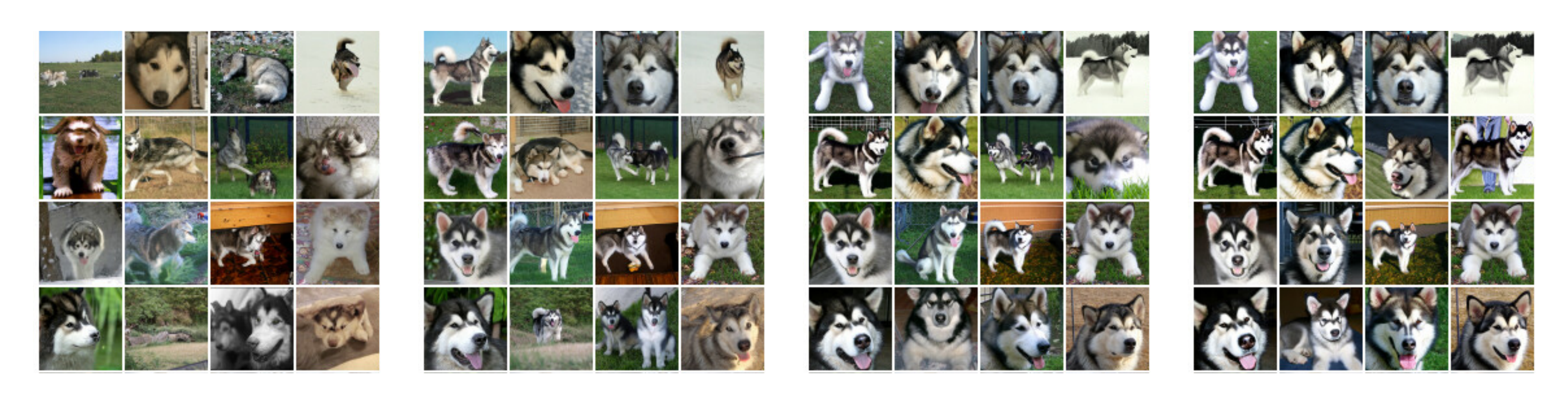
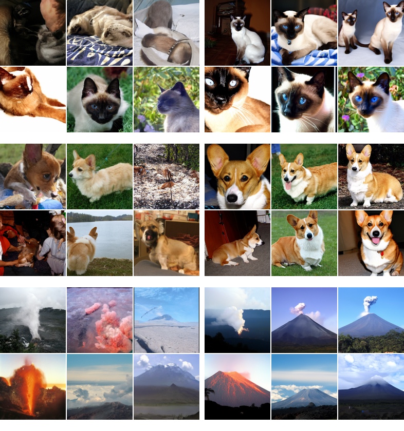
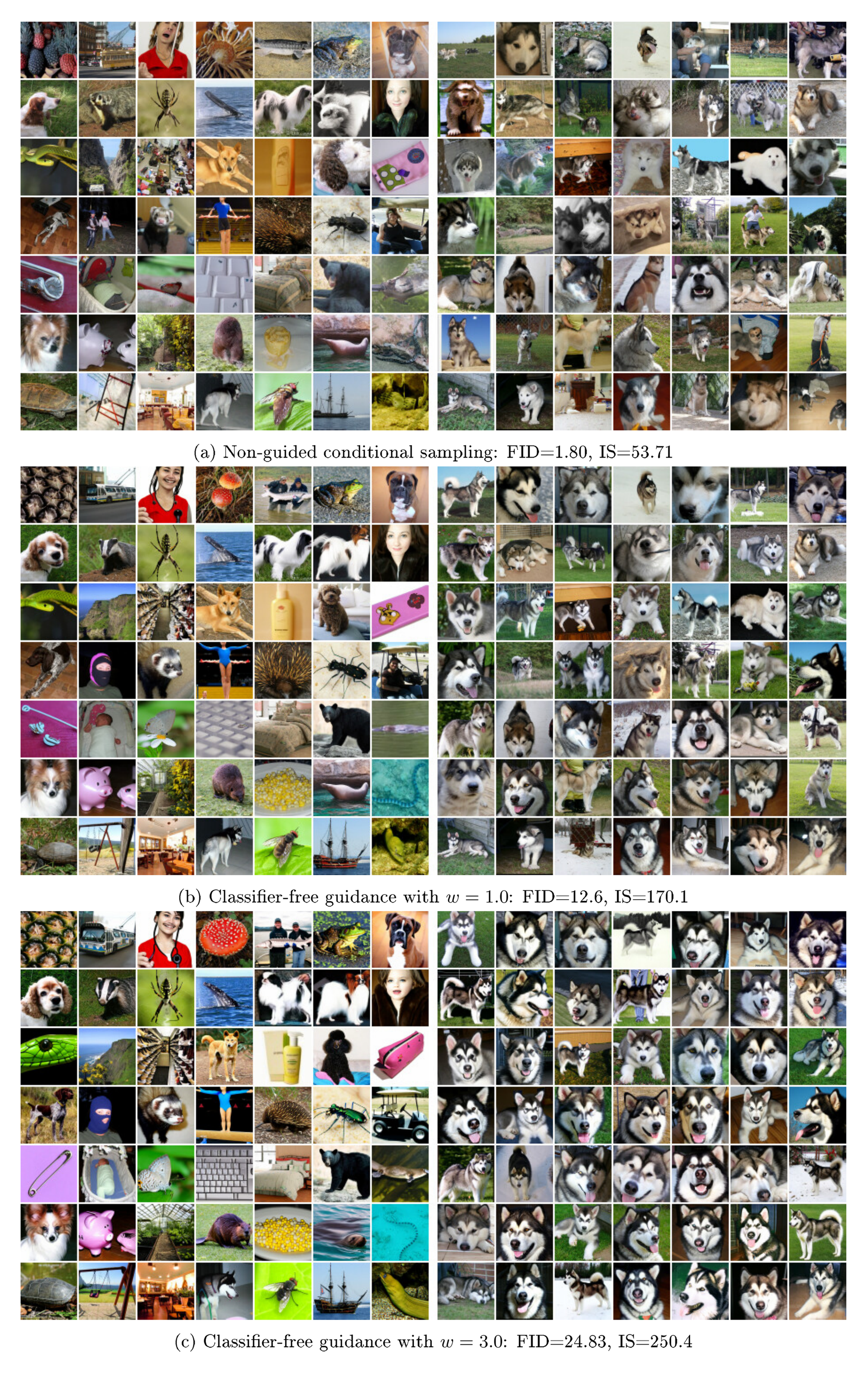
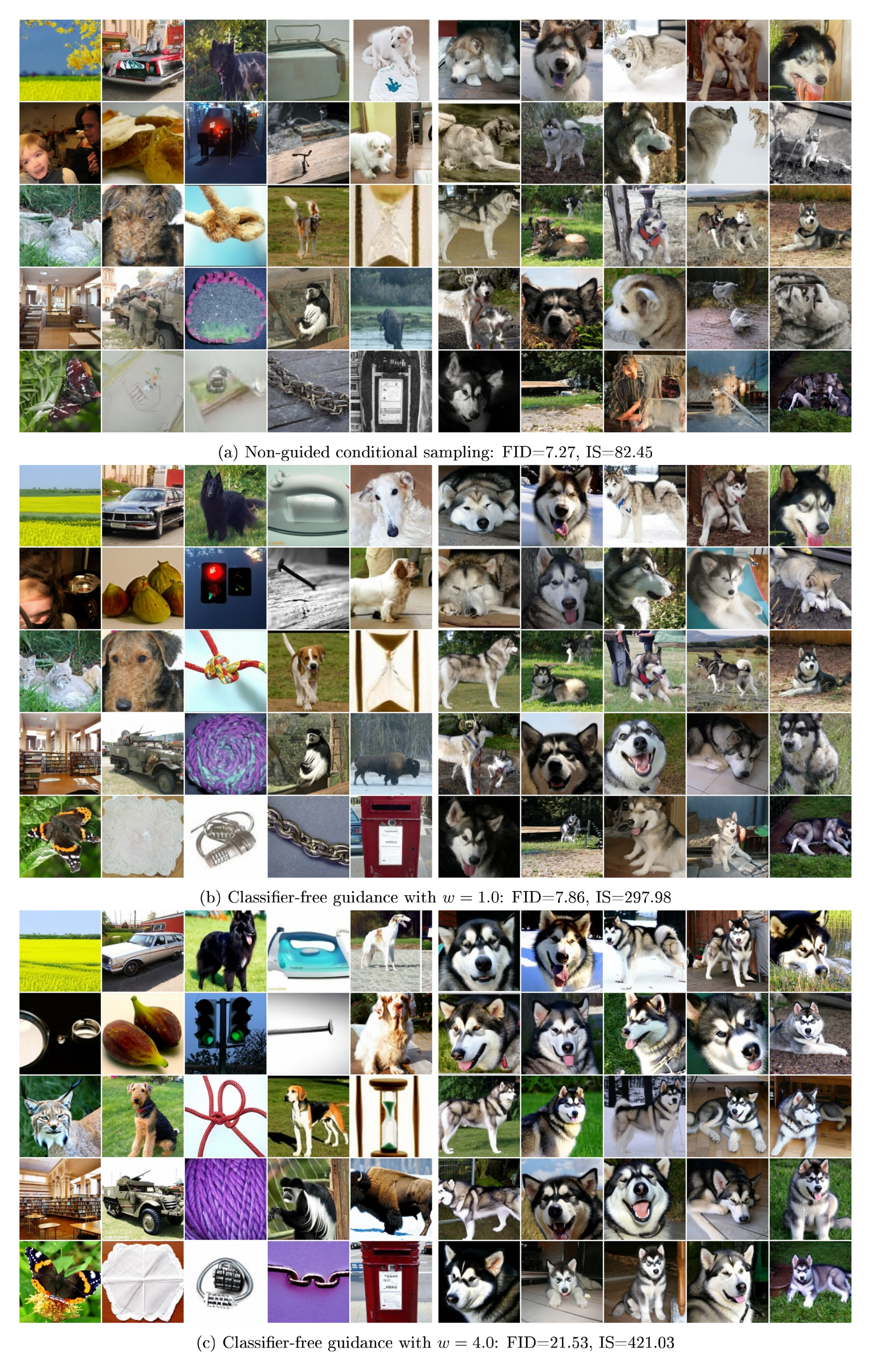
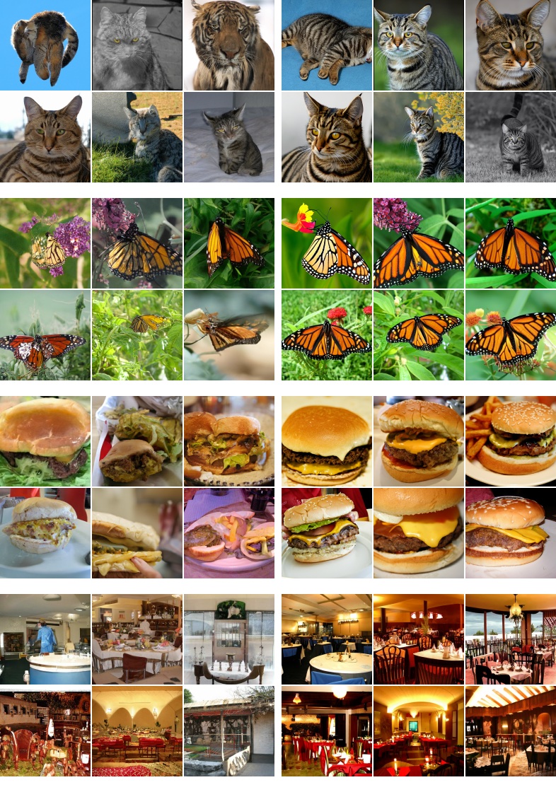
Figure 1, Figure 6, Figure 3, Figure 7, and Figure 8 show randomly generated samples from our model for different levels of guidance: here we clearly see that increasing classifier-free guidance strength has the expected effect of decreasing sample variety and increasing individual sample fidelity.

:::

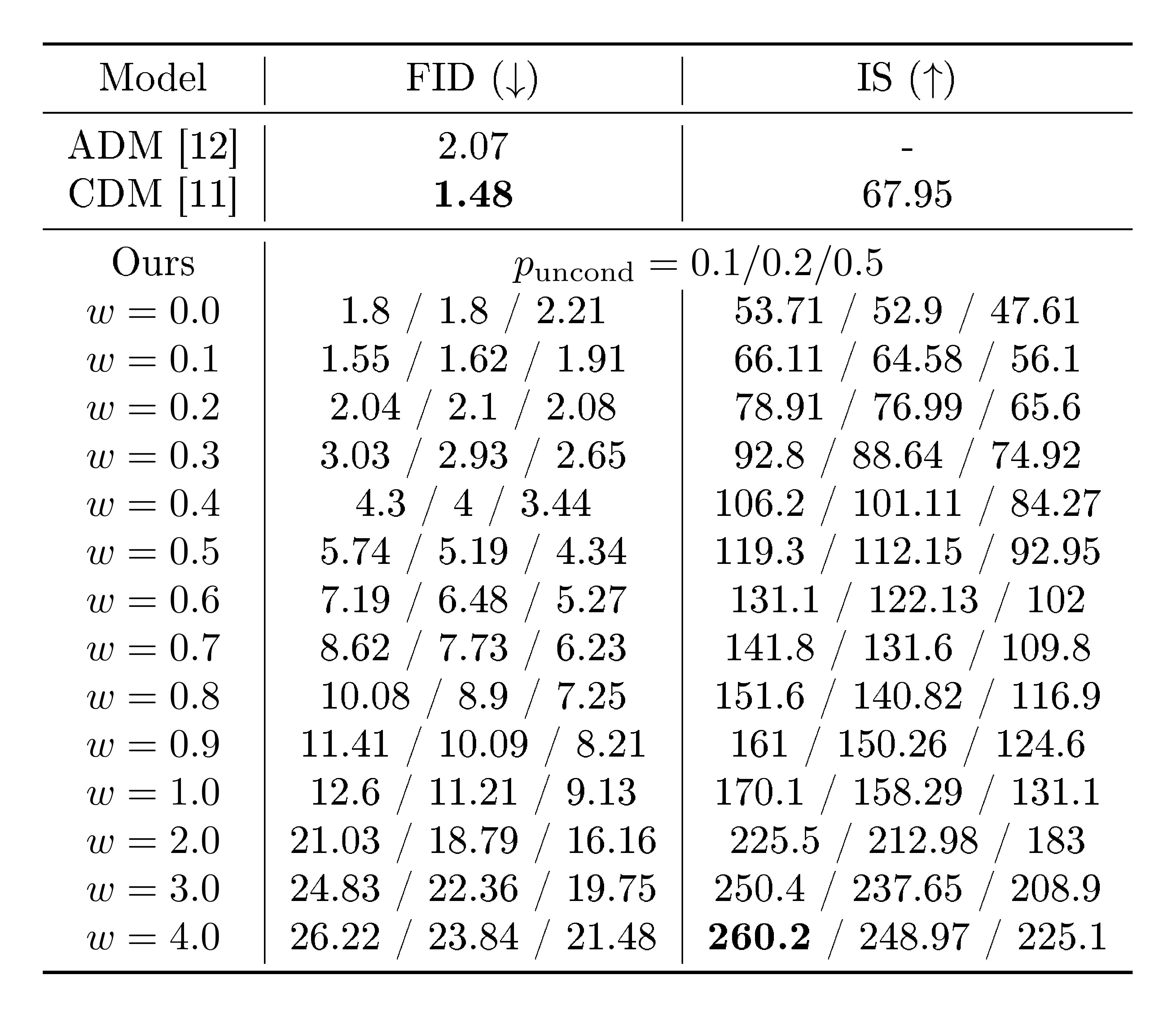
Table 1: ImageNet 64x64 results ($w=0.0$ refers to non-guided models).

:::

4.2 Varying the unconditional training probability

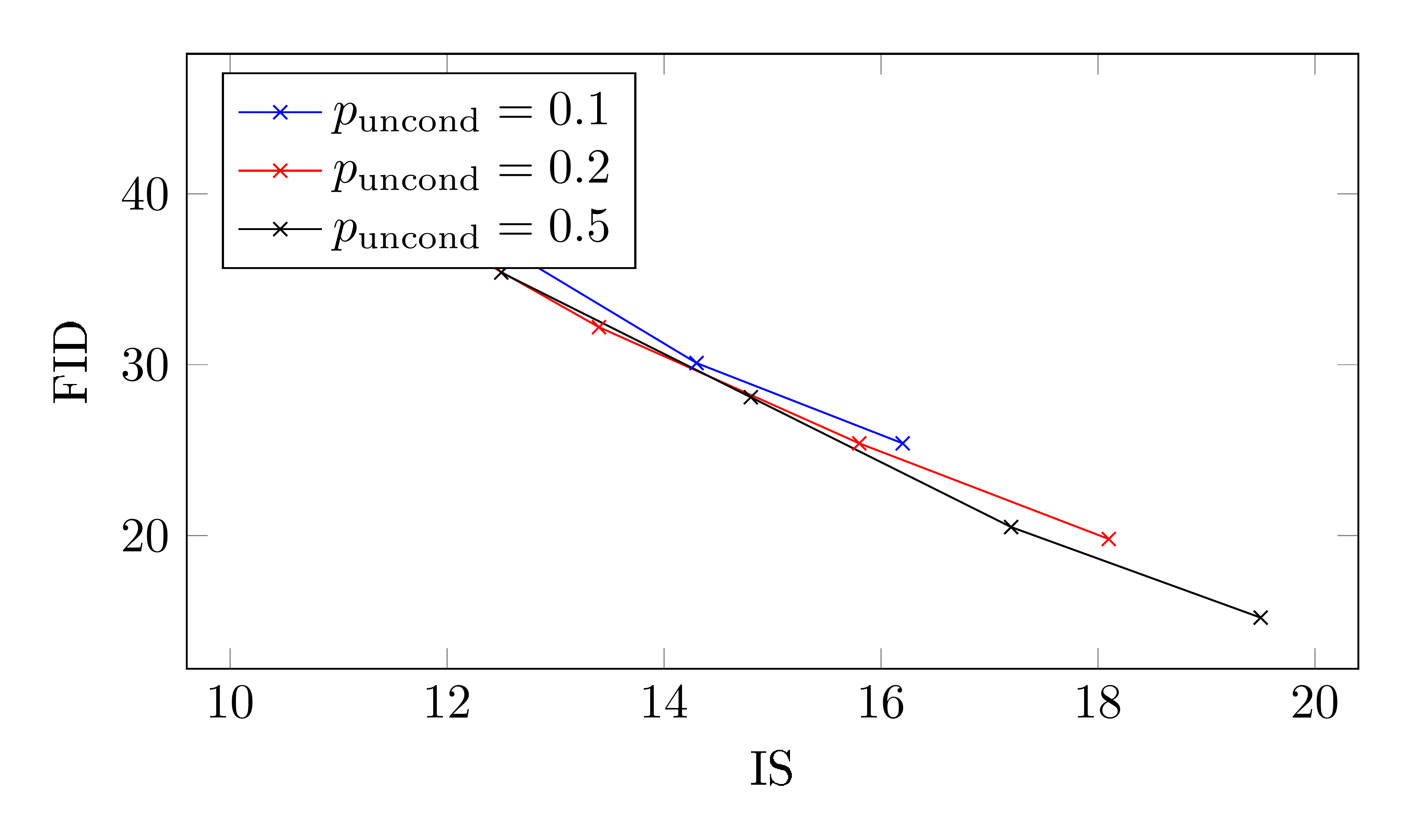
The main hyperparameter of classifier-free guidance at training time is $p_\mathrm{uncond}$, the probability of training on unconditional generation during joint training of the conditional and unconditional diffusion models. Here, we study the effect of training models on varying $p_\mathrm{uncond}$ on $64\times64$ ImageNet.

Table 1 and Figure 4 show the effects of $p_\mathrm{uncond}$ on sample quality. We trained models with $p_\mathrm{uncond}\in{0.1, 0.2, 0.5}$, all for 400 thousand training steps, and evaluated sample quality across various guidance strengths. We find $p_\mathrm{uncond}=0.5$ consistently performs worse than $p_\mathrm{uncond}\in{0.1, 0.2}$ across the entire IS/FID frontier; $p_\mathrm{uncond}\in{0.1, 0.2}$ perform about equally as well as each other.

Based on these findings, we conclude that only a relatively small portion of the model capacity of the diffusion model needs to be dedicated to the unconditional generation task in order to produce classifier-free guided scores effective for sample quality. Interestingly, for classifier guidance, [12] report that relatively small classifiers with little capacity are sufficient for effective classifier guided sampling, mirroring this phenomenon that we found with classifier-free guided models.

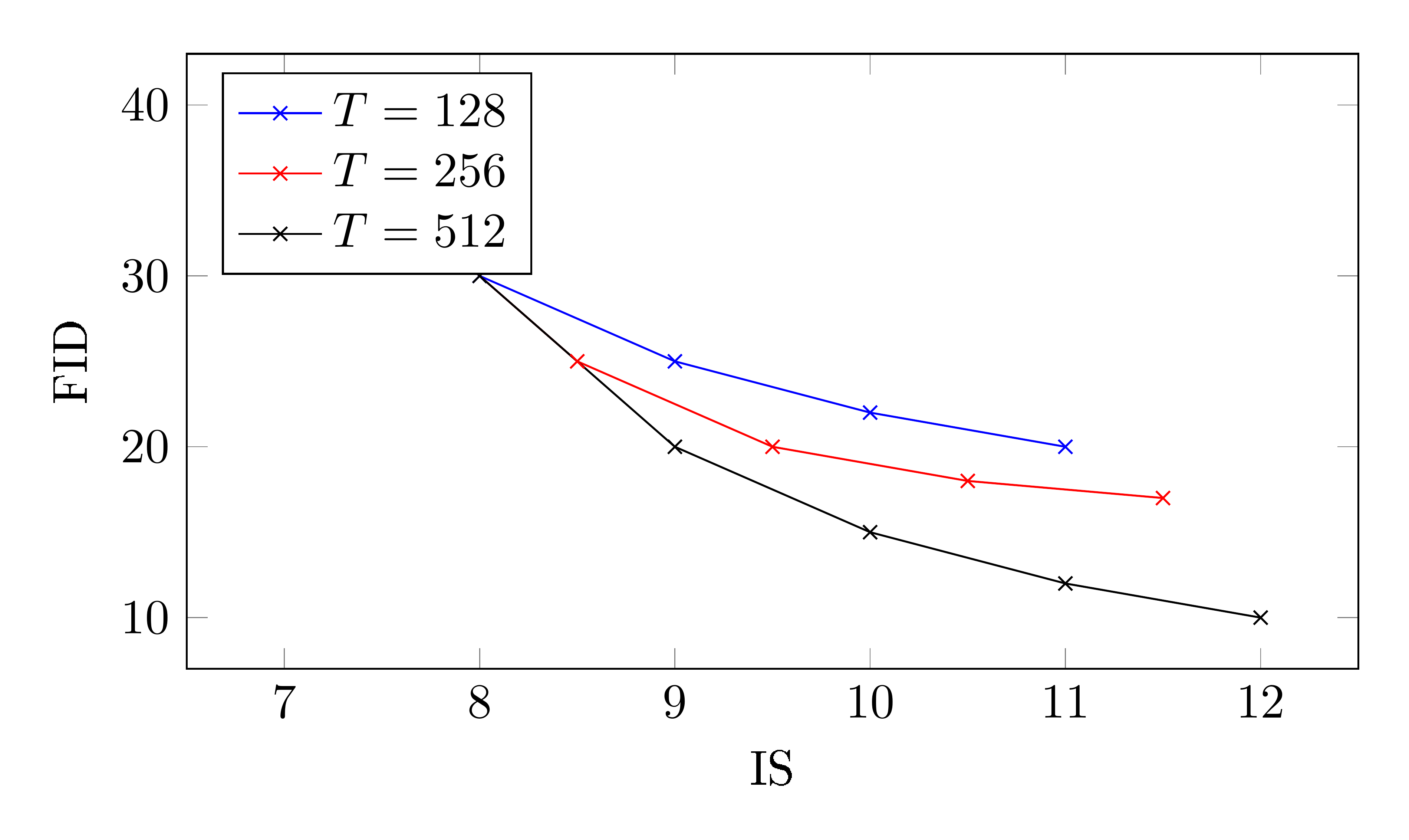
4.3 Varying the number of sampling steps

Since the number of sampling steps $T$ is known to have a major impact on the sample quality of a diffusion model, here we study the effect of varying $T$ on our $128\times128$ ImageNet model. Table 2 and Figure 5 show the effect of varying $T\in{128, 256, 1024}$ over a range of guidance strengths. As expected, sample quality improves when $T$ is increased, and for this model $T=256$ attains a good balance between sample quality and sampling speed.

Note that $T=256$ is approximately the same number of sampling steps used by ADM-G ([12]), which is outperformed by our model. However, it is important to note that each sampling step for our method requires evaluating the denoising model twice, once for the conditional ${\boldsymbol{\epsilon}}\theta(\mathbf{z}\lambda, \mathbf{c})$ and once for the unconditional ${\boldsymbol{\epsilon}}\theta(\mathbf{z}\lambda)$. Because we used the same model architecture as ADM-G, the fair comparison in terms of sampling speed would be our $T=128$ setting, which underperforms compared to ADM-G in terms of FID score.

:::

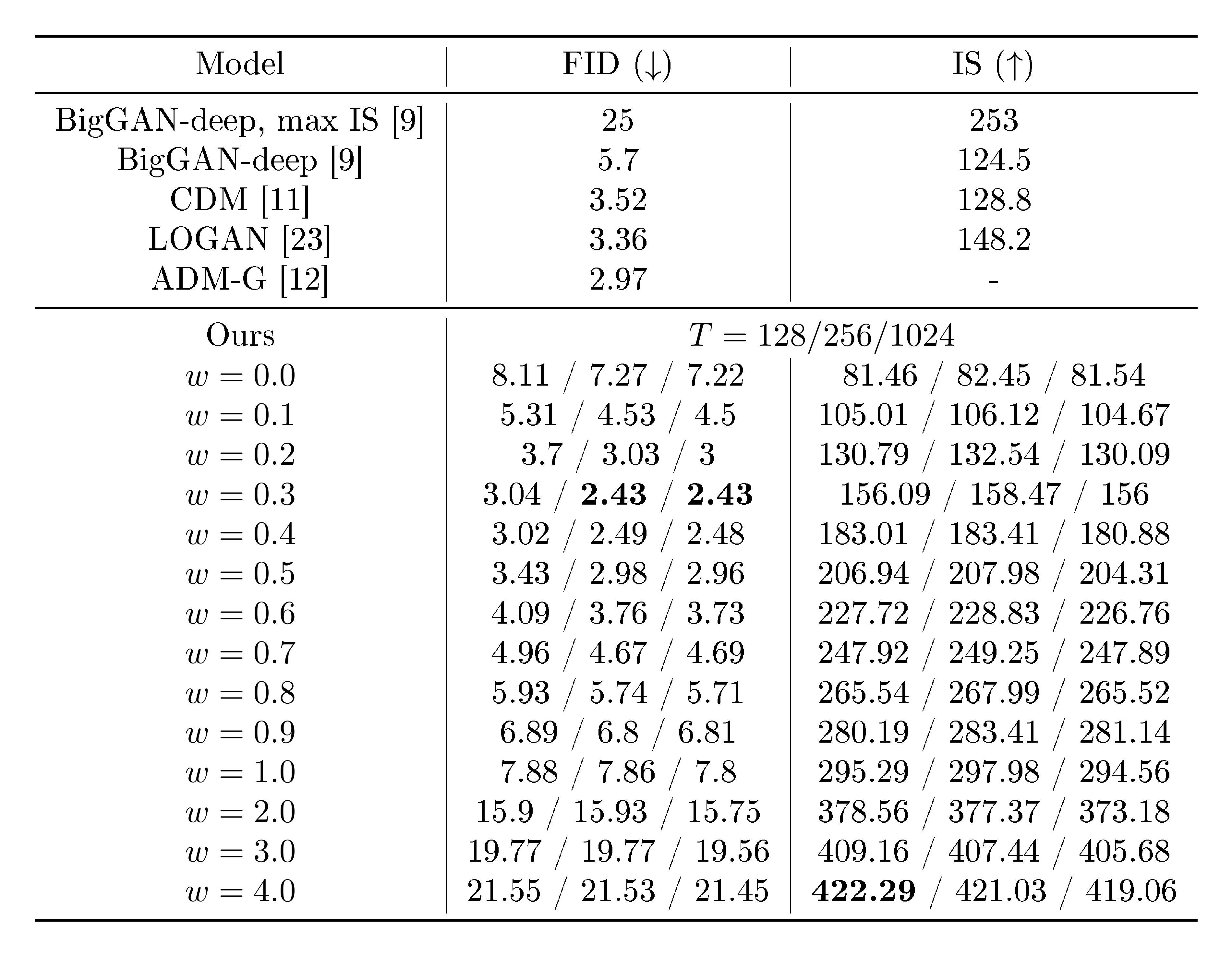
Table 2: ImageNet 128x128 results ($w=0.0$ refers to non-guided models).

:::

5. Discussion

Section Summary: The classifier-free guidance method stands out for its simplicity, requiring just a single line of code to randomly drop conditioning during training and blend conditional and unconditional scores during sampling, unlike classifier guidance which needs a separate, complex classifier trained on noisy data. This approach allows pure generative models to balance image quality metrics without adversarial effects on classifiers and works by boosting conditional likelihood while reducing unconditional likelihood through a novel negative score term. While it can sometimes skip training an unconditional model by summing over known class distributions, it may slow sampling due to extra model passes, and future improvements could address the trade-off between higher fidelity and reduced sample diversity to avoid biases in real-world applications.

The most practical advantage of our classifier-free guidance method is its extreme simplicity: it is only a one-line change of code during training—to randomly drop out the conditioning—and during sampling—to mix the conditional and unconditional score estimates. Classifier guidance, by contrast, complicates the training pipeline since it requires training an extra classifier. This classifier must be trained on noisy $\mathbf{z}_\lambda$, so it is not possible to plug in a standard pre-trained classifier.

Since classifier-free guidance is able to trade off IS and FID like classifier guidance without needing an extra trained classifier, we have demonstrated that guidance can be performed with a pure generative model. Furthermore, our diffusion models are parameterized by unconstrained neural networks and therefore their score estimates do not necessarily form conservative vector fields, unlike classifier gradients ([22]). Therefore, our classifier-free guided sampler follows step directions that do not resemble classifier gradients at all and thus cannot be interpreted as a gradient-based adversarial attack on a classifier, and hence our results show that boosting the classifier-based IS and FID metrics can be accomplished with pure generative models with a sampling procedure that is not adversarial against image classifiers using classifier gradients.

We also have arrived at an intuitive explanation for how guidance works: it decreases the unconditional likelihood of the sample while increasing the conditional likelihood. Classifier-free guidance accomplishes this by decreasing the unconditional likelihood with a negative score term, which to our knowledge has not yet been explored and may find uses in other applications.

Classifier-free guidance as presented here relies on training an unconditional model, but in some cases this can be avoided. If the class distribution is known and there are only a few classes, we can use the fact that $\sum_\mathbf{c} p(\mathbf{x}| \mathbf{c}) p(\mathbf{c}) = p(\mathbf{x})$ to obtain an unconditional score from conditional scores without explicitly training for the unconditional score. Of course, this would require as many forward passes as there are possible values of $\mathbf{c}$ and would be inefficient for high dimensional conditioning.

A potential disadvantage of classifier-free guidance is sampling speed. Generally, classifiers can be smaller and faster than generative models, so classifier guided sampling may be faster than classifier-free guidance because the latter needs to run two forward passes of the diffusion model, one for conditional score and another for the unconditional score. The necessity to run multiple passes of the diffusion model might be mitigated by changing the architecture to inject conditioning late in the network, but we leave this exploration for future work.

Finally, any guidance method that increases sample fidelity at the expense of diversity must face the question of whether decreased diversity is acceptable. There may be negative impacts in deployed models, since sample diversity is important to maintain in applications where certain parts of the data are underrepresented in the context of the rest of the data. It would be an interesting avenue of future work to try to boost sample quality while maintaining sample diversity.

6. Conclusion

Section Summary: This conclusion introduces classifier-free guidance as a technique for diffusion models that boosts the quality of generated samples while reducing their variety. It works like traditional classifier guidance but without needing an actual classifier, and the results prove that these models can achieve top-notch quality scores on their own, without relying on classifier-related math. The authors are excited for future tests of this method across more scenarios and types of data.

We have presented classifier-free guidance, a method to increase sample quality while decreasing sample diversity in diffusion models. Classifier-free guidance can be thought of as classifier guidance without a classifier, and our results showing the effectiveness of classifier-free guidance confirm that pure generative diffusion models are capable of maximizing classifier-based sample quality metrics while entirely avoiding classifier gradients. We look forward to further explorations of classifier-free guidance in a wider variety of settings and data modalities.

7. Acknowledgements

We thank Ben Poole and Mohammad Norouzi for discussions.

Appendix

A. Samples

References

Section Summary: This section lists key research papers on generative AI models, focusing on techniques like diffusion models and score-based methods that help computers create realistic images, audio, and other data from scratch. It includes foundational works on unsupervised learning, such as those using nonequilibrium thermodynamics and gradient estimation, alongside advancements in models like WaveGrad for sound synthesis and DiffWave for versatile audio generation. The references also cover comparisons with GANs, improvements in training, and evaluations on large datasets like ImageNet, spanning from 2004 to 2021.

[1] Jascha Sohl-Dickstein, Eric Weiss, Niru Maheswaranathan, and Surya Ganguli. Deep unsupervised learning using nonequilibrium thermodynamics. In International Conference on Machine Learning, pp.\ 2256–2265, 2015.

[2] Yang Song and Stefano Ermon. Generative modeling by estimating gradients of the data distribution. In Advances in Neural Information Processing Systems, pp.\ 11895–11907, 2019.

[3] Jonathan Ho, Ajay Jain, and Pieter Abbeel. Denoising diffusion probabilistic models. In Advances in Neural Information Processing Systems, pp.\ 6840–6851, 2020.

[4] Yang Song, Jascha Sohl-Dickstein, Diederik P Kingma, Abhishek Kumar, Stefano Ermon, and Ben Poole. Score-based generative modeling through stochastic differential equations. International Conference on Learning Representations, 2021b.

[5] Diederik P Kingma, Tim Salimans, Ben Poole, and Jonathan Ho. Variational diffusion models. arXiv preprint arXiv:2107.00630, 2021.

[6] Yang Song, Conor Durkan, Iain Murray, and Stefano Ermon. Maximum likelihood training of score-based diffusion models. arXiv e-prints, pp.\ arXiv–2101, 2021a.

[7] Nanxin Chen, Yu Zhang, Heiga Zen, Ron J Weiss, Mohammad Norouzi, and William Chan. WaveGrad: Estimating gradients for waveform generation. International Conference on Learning Representations, 2021.

[8] Zhifeng Kong, Wei Ping, Jiaji Huang, Kexin Zhao, and Bryan Catanzaro. DiffWave: A Versatile Diffusion Model for Audio Synthesis. International Conference on Learning Representations, 2021.

[9] Andrew Brock, Jeff Donahue, and Karen Simonyan. Large scale GAN training for high fidelity natural image synthesis. In International Conference on Learning Representations, 2019.

[10] Ali Razavi, Aaron van den Oord, and Oriol Vinyals. Generating diverse high-fidelity images with VQ-VAE-2. In Advances in Neural Information Processing Systems, pp.\ 14837–14847, 2019.

[11] Jonathan Ho, Chitwan Saharia, William Chan, David J Fleet, Mohammad Norouzi, and Tim Salimans. Cascaded diffusion models for high fidelity image generation. arXiv preprint arXiv:2106.15282, 2021.

[12] Prafulla Dhariwal and Alex Nichol. Diffusion models beat GANs on image synthesis. arXiv preprint arXiv:2105.05233, 2021.

[13] Diederik P Kingma and Prafulla Dhariwal. Glow: Generative flow with invertible 1x1 convolutions. In Advances in Neural Information Processing Systems, pp.\ 10215–10224, 2018.

[14] Tim Salimans, Ian Goodfellow, Wojciech Zaremba, Vicki Cheung, Alec Radford, and Xi Chen. Improved techniques for training GANs. In Advances in Neural Information Processing Systems, pp.\ 2234–2242, 2016.

[15] Martin Heusel, Hubert Ramsauer, Thomas Unterthiner, Bernhard Nessler, and Sepp Hochreiter. GANs trained by a two time-scale update rule converge to a local Nash equilibrium. In Advances in Neural Information Processing Systems, pp.\ 6626–6637, 2017.

[16] Alex Nichol and Prafulla Dhariwal. Improved denoising diffusion probabilistic models. International Conference on Machine Learning, 2021.

[17] Pascal Vincent. A connection between score matching and denoising autoencoders. Neural Computation, 23(7):1661–1674, 2011.

[18] Aapo Hyvärinen and Peter Dayan. Estimation of non-normalized statistical models by score matching. Journal of Machine Learning Research, 6(4), 2005.

[19] Yves Grandvalet and Yoshua Bengio. Semi-supervised learning by entropy minimization. In Proceedings of the 17th International Conference on Neural Information Processing Systems, pp.\ 529–536, 2004.

[20] Peter Grünwald and John Langford. Suboptimal behavior of bayes and mdl in classification under misspecification. Machine Learning, 66(2-3):119–149, 2007.

[21] Olga Russakovsky, Jia Deng, Hao Su, Jonathan Krause, Sanjeev Satheesh, Sean Ma, Zhiheng Huang, Andrej Karpathy, Aditya Khosla, Michael Bernstein, et al. ImageNet large scale visual recognition challenge. International Journal of Computer Vision, 115(3):211–252, 2015.

[22] Tim Salimans and Jonathan Ho. Should EBMs model the energy or the score? In Energy Based Models Workshop-ICLR 2021, 2021.