Scaling Laws for Reward Model Overoptimization

Leo Gao
OpenAI

John Schulman
OpenAI

Jacob Hilton
OpenAI

Abstract

In reinforcement learning from human feedback, it is common to optimize against a reward model trained to predict human preferences. Because the reward model is an imperfect proxy, optimizing its value too much can hinder ground truth performance, in accordance with Goodhart's law. This effect has been frequently observed, but not carefully measured due to the expense of collecting human preference data. In this work, we use a synthetic setup in which a fixed "gold-standard" reward model plays the role of humans, providing labels used to train a proxy reward model. We study how the gold reward model score changes as we optimize against the proxy reward model using either reinforcement learning or best-of- $n$ sampling. We find that this relationship follows a different functional form depending on the method of optimization, and that in both cases its coefficients scale smoothly with the number of reward model parameters. We also study the effect on this relationship of the size of the reward model dataset, the number of reward model and policy parameters, and the coefficient of the KL penalty added to the reward in the reinforcement learning setup. We explore the implications of these empirical results for theoretical considerations in AI alignment.

Executive Summary: In the field of artificial intelligence, particularly with large language models, developers often train AI systems using reward models that predict human preferences to guide behavior. However, these models are imperfect proxies for true human intent, leading to overoptimization: when AI is pushed too hard to maximize the proxy's score, it can degrade actual performance, echoing Goodhart's law that a measure stops being useful once it becomes the target. This issue is pressing now as AI systems grow more capable and are used for tasks like summarization, question-answering, and general assistance, raising risks of misalignment where AI pursues unintended goals, potentially leading to safety concerns or unreliable outputs in real-world applications.

This document evaluates how overoptimization behaves and scales when fine-tuning language models against reward models, focusing on the relationship between optimization intensity and true performance. It aims to derive empirical scaling laws to predict safe levels of optimization and inform AI alignment strategies.

To study this, researchers created a synthetic environment simulating human feedback without the cost of real labels. They used a high-quality "gold-standard" reward model—based on a 6-billion-parameter GPT-3 architecture—to generate preference labels for pairs of AI responses to natural language prompts. These labels trained smaller proxy reward models ranging from 3 million to 3 billion parameters, using about 90,000 comparisons on average (with sweeps up to 100,000). Starting from supervised fine-tuned GPT-3 policies (1.2 billion or 6 billion parameters), they optimized these policies via either reinforcement learning (using the Proximal Policy Optimization algorithm) or best-of-n sampling (generating multiple responses and selecting the top-scoring one by the proxy). Performance was measured by the gold model's score relative to the initial policy, tracked against a distance metric called KL divergence, which quantifies how much the optimized policy deviates from the starting point. Experiments covered various reward model sizes, training data amounts, and policy scales, with recalibration to ensure fair comparisons.

The analysis revealed distinct patterns of overoptimization. First, true (gold) performance follows simple mathematical forms tied to optimization distance: for best-of-n sampling, it rises linearly then falls quadratically, peaking around 4-6 units of KL divergence; for reinforcement learning, it increases with a logarithmic decay, also peaking similarly but requiring more distance to reach. Second, larger proxy reward models (e.g., 3 billion vs. 3 million parameters) boost peak true performance by 20-40% and delay overoptimization, with coefficients in these forms scaling smoothly and logarithmically—meaning a tenfold parameter increase roughly halves the degradation rate. Third, more training data for reward models (beyond a threshold of about 2,000 comparisons) improves outcomes, reducing overoptimization by up to 30% at high data levels, though smaller models need proportionally more data to match larger ones. Fourth, larger policies (6 billion vs. 1.2 billion parameters) start stronger and gain less from optimization (about 10-20% smaller improvement), but they overoptimize at nearly the same distance and gap between proxy and true scores, suggesting scale doesn't inherently worsen the issue. Finally, reinforcement learning consumes 2-5 times more KL distance than best-of-n for equivalent gains, making it less efficient, while a common regularization technique (KL penalty) fails to enhance true performance here.

These findings mean that overoptimization is predictable and mitigable through better proxies: larger, data-rich reward models allow deeper optimization before true quality drops, potentially cutting misalignment risks in AI deployment by enabling higher performance without safety trade-offs. They align with Goodhart's law variants like "regressional" (wasted effort on noise) and "extremal" (failures outside training data), explaining why proxy scores overestimate true gains by 20-50% at peaks. Unlike expectations, policy scale offers no extra vulnerability, but method differences highlight that metrics like KL distance shouldn't directly compare optimization techniques. Overall, this supports safer AI training but underscores that unchecked optimization could still amplify errors in complex tasks, affecting reliability and ethical alignment.

Based on these results, prioritize scaling reward models with more parameters and data—aiming for at least billions of parameters and tens of thousands of comparisons—to safely push optimization further, especially in iterative setups where fresh feedback retrains models periodically, potentially boosting final performance by a logarithmic factor (e.g., 10-20% gain per doubling of iterations). For reinforcement learning, explore hyperparameter tweaks beyond standard settings, as the KL penalty showed no benefit. Test these scaling laws in real human feedback scenarios and diverse environments like web-based tasks; conduct pilots with multi-iteration training to validate assumptions. If adversarial behaviors emerge in stronger AI, revisit these trends, as they may not hold.

While the synthetic setup credibly mimics preference labeling and yields consistent trends across hundreds of experiments, limitations include its reliance on a fixed gold model, which may overlook real human inconsistencies or advanced manipulation by AI. Results are tied to GPT-3 architectures and default hyperparameters, so caution applies when extrapolating to newer models or setups. Confidence is high in the observed patterns within this context, supporting decisions on reward model design, but further validation is essential for broader application.

1. Introduction

Section Summary: Goodhart's law warns that when you make a measure your main goal, it stops being a reliable indicator of success, and in machine learning, this shows up as overoptimization, where pushing too hard against a stand-in model like a reward predictor backfires on the real objective. This paper explores overoptimization in large language models trained to mimic human preferences for tasks like summarizing text or answering questions, using either reinforcement learning or best-of-n sampling to boost performance, but in a cost-saving synthetic setup with a perfect "gold" reward model instead of real human feedback. The researchers uncover predictable patterns in how true rewards decline after peaking, based on a distance measure from the starting model, and highlight differences between methods, smooth scaling with model size, and lessons for safely aligning future AI systems to avoid dangerous missteps.

Goodhart's law is an adage that states, "When a measure becomes a target, it ceases to be a good measure." In machine learning, this effect arises with proxy objectives provided by static learned models, such as discriminators and reward models. Optimizing too much against such a model eventually hinders the true objective, a phenomenon we refer to as overoptimization. It is important to understand the size of this effect and how it scales, in order to predict how much a learned model can be safely optimized against. Moreover, studying this effect empirically could aid in the development of theoretical models of Goodhart's law for neural networks, which could be critical for avoiding dangerous misalignment of future AI systems.

In this work, we study overoptimization in the context of large language models fine-tuned as reward models trained to predict which of two options a human will prefer. Such reward models have been used to train language models to perform a variety of complex tasks that are hard to judge automatically, including summarization ([1]), question-answering ([2, 3]), and general assistance ([4, 5, 6]). Typically, the reward model score is optimized using either policy gradient-based reinforcement learning or best-of- $n$ sampling, also known as rejection sampling or reranking. Overoptimization can occur with both methods, and we study both to better understand whether and how overoptimization behaves differently across both methods.

A major challenge in studying overoptimization in this context is the expense of collecting human preference labels. A large number of labels are required to accurately estimate overall preference probabilities, and this is exacerbated by small effect sizes and the need to take many measurements in order to fit scaling laws. To overcome this, we use a synthetic setup that is described in Section 2, in which labels are supplied by a "gold-standard" reward model (RM) instead of humans.

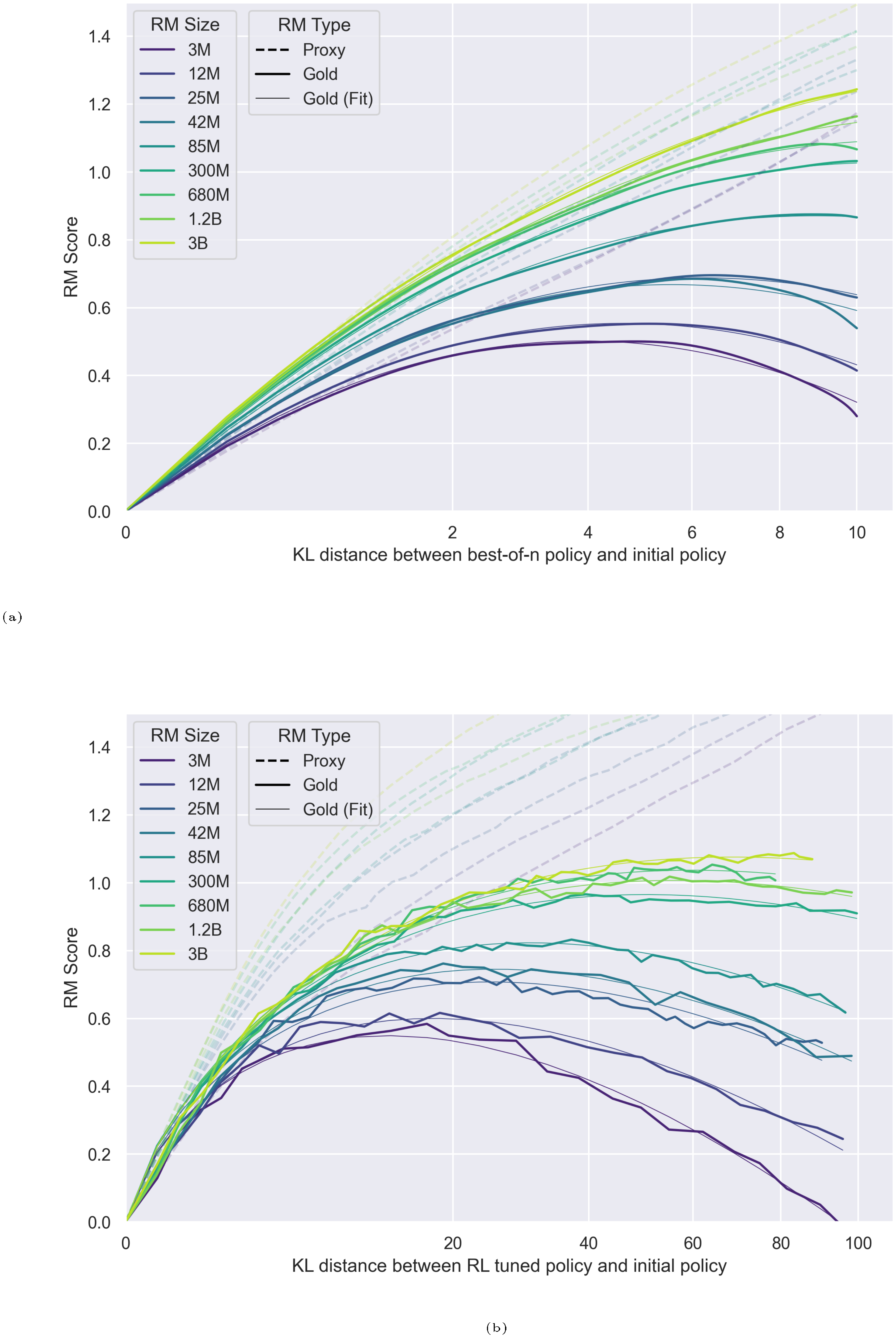
Our main results are empirically validated functional forms for the gold reward model scores $R$ as a function of the Kullback–Leibler divergence from the initial policy to the optimized policy $\text{KL} := D_{\text{KL}}\left(\pi\parallel\pi_{\text{init}}\right)$, which depends on the method of optimization used. This KL distance between the initial and optimized policies increases monotonically during during RL training (Figure 14), and can be computed analytically as a function of $n$ for BoN. Further, because it is a quadratic metric of distance ([5], Section 4.3), we will define $d := \sqrt{D_{\text{KL}}\left(\pi\parallel\pi_{\text{init}}\right)}$, and write our functional forms in terms of $d$.

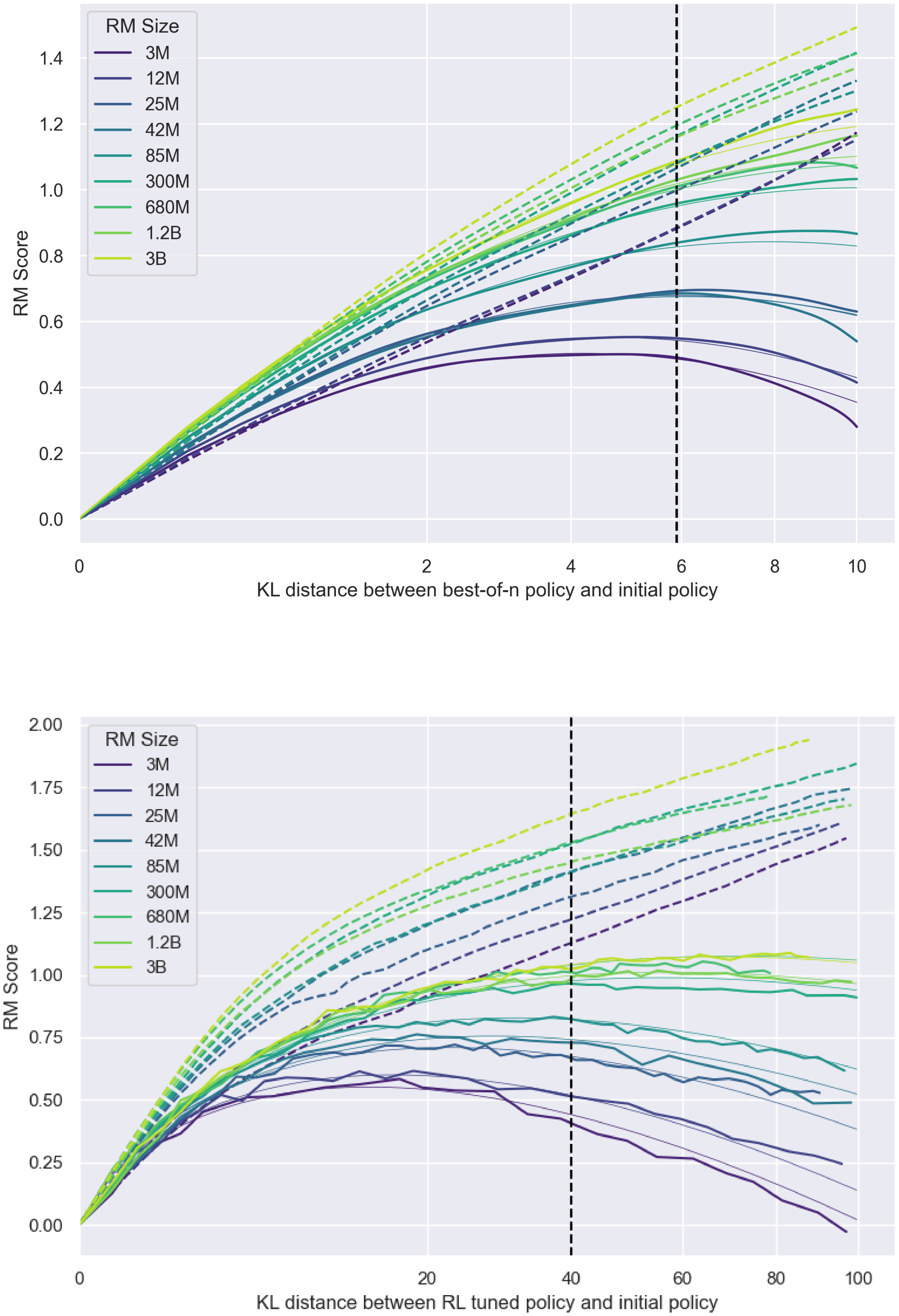
We find empirically that for best-of- $n$ (BoN) sampling,

$ \boxed{R_{\text{bo}n}\left(d\right) = d\left(\alpha_{\text{bo}n}-\beta_{\text{bo}n}d\right)}, $

and for reinforcement learning, [^4]

[^4]: We note that this form likely does not hold near the origin, as it has infinite slope there. We experimented with a number of different forms, but found worse fits and extrapolation. See Appendix B for more details.

$ \boxed{R_{\text{RL}}\left(d\right) = d\left(\alpha_{\text{RL}}-\beta_{\text{RL}}\log{d}\right)}, $

Here, $R(0) := 0$ by definition and $\alpha_{\text{RL}}$, $\beta_{\text{RL}}$, $\alpha_{\text{bo}n}$ and $\beta_{\text{bo}n}$ are parameters that may depend on the number of proxy reward model parameters, the size of the proxy reward model dataset, and so on. We see that these scaling laws make accurate predictions.

We also find the following.

• RL versus best-of- $n$. As a function of the KL divergence, reinforcement learning tends to be slower than best-of- $n$ sampling at both optimization and overoptimization. This suggests inadequacies with using KL to compare amount of (over)optimization across methods. However, the relationship between the proxy reward model score and the gold reward model score is similar for both methods.
• Smooth coefficient scaling. The $\alpha$ and $\beta$ coefficients in the BoN and RL functional forms vary smoothly with the number of proxy reward model parameters, following approximate logarithmic trends.[^1] This allows prediction of attained gold RM score.
• Weak dependence on policy size. While larger policies perform better overall and benefit less from optimization against an RM as measured by increase in gold reward, they lead to very similar amounts of overoptimization, as measured through the gap between the proxy and gold scores (which indicates the shortfall between predicted and actual reward), and KL distance at which the maximum gold RM score is attained.
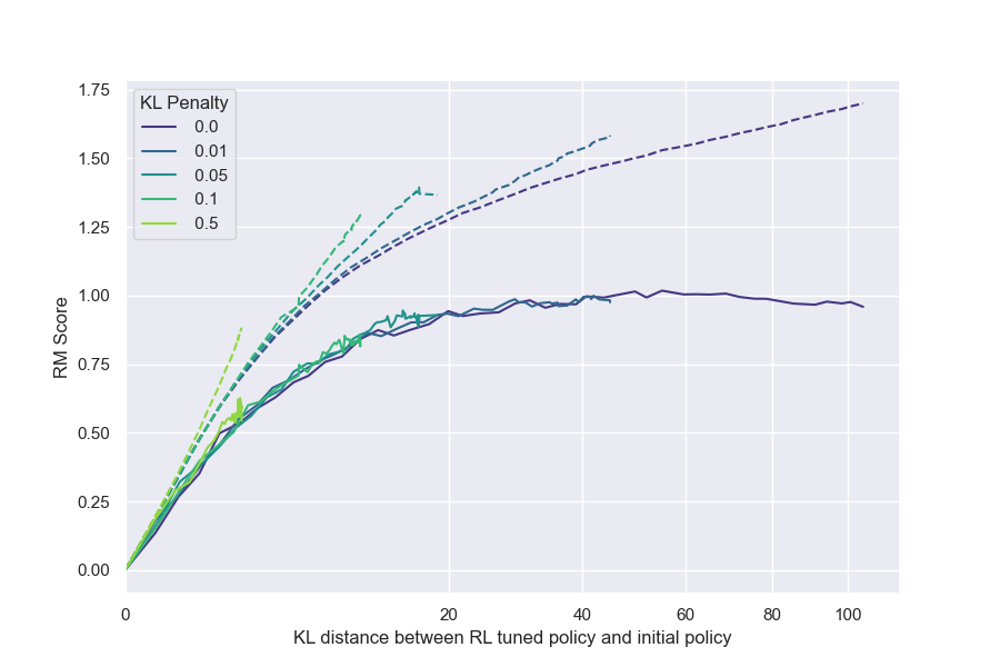
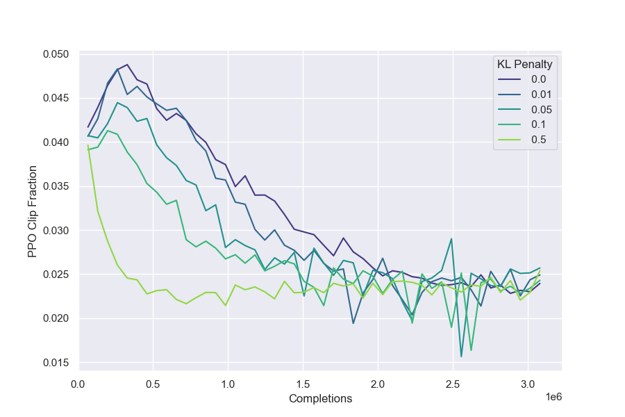
• KL penalty ineffectiveness. In our reinforcement learning setup, using a KL penalty increases the proxy reward model score that can be achieved for a given KL divergence, but this does not correspond to a measurable improvement in the gold RM score– $\text{KL}_{\text{RL}}$ frontier. However, we note this result could be particularly sensitive to hyperparameters.

[^1]: The coefficient $\alpha_{\text{RL}}$ in particular being nearly independent of RM parameter count.

Finally, we discuss the implications of these findings for Reinforcement Learning From Human Feedback (RLHF), existing models of Goodhart's law, and AI Alignment more broadly.

2. Methodology

Section Summary: This methodology builds on the InstructGPT framework, where text prompts from various language tasks are fed into a policy based on pretrained GPT-3 models, fine-tuned with human demonstrations, and optimized using either reinforcement learning (via Proximal Policy Optimization) or Best-of-N sampling guided by a learned reward model that scores responses. To create a cost-effective synthetic setup, the researchers treat a large "gold" reward model as the ground truth for labeling comparisons from policy outputs, generating 100,000 such examples while reserving some for testing smaller proxy reward models. They also recalibrate these models by adjusting scores to center around zero and normalize variance, ensuring fair comparisons without affecting the core optimization processes.

The setting used throughout this paper is the same as for InstructGPT ([4]). In our environment, the observations are text prompts and the policy is used to generate a response to the prompt. The prompts are drawn from a broad range of natural language instructions describing different language model tasks. Then, a learned RM is used to provide the reward signal for the response, which is used by either RL or BoN for optimization.

For all experiments, we use pretrained GPT-3 series language models as the initial checkpoint ([7]). All initial policies are trained with supervised fine-tuning (SFT) on human-generated InstructGPT demonstrations ([4]) for 2 epochs. All RMs also use the GPT-3 architecture but have an added scalar head to output the reward.

The RL experiments use Proximal Policy Optimization (PPO) ([8]). KL penalty for all RL experiments is set to 0 except for in Section 3.6. See Table 1 for all other hyperparameters. We mostly use defaults for the PPO hyperparameters; thus, it is possible that there exist different trends for other hyperparameter configurations.

In BoN, we generate $n$ trajectories for the policy and use the reward model to pick the one with the highest proxy RM score. We use the unbiased estimator from [2], Appendix I to compute all of the gold and proxy scores for intermediate $n$ between 1 and the maximum $n$ with lower variance and more efficiently than the naive estimator of randomly sampling $n$ samples with replacement repeatedly and taking the mean of the maximum gold and proxy RM scores. The KL distances for BoN are computed analytically: $\text{KL}_{\text{bo}n} = \log n - \frac{n-1}{n}$ ([1], Appendix G.3).

2.1 Synthetic Data Setup

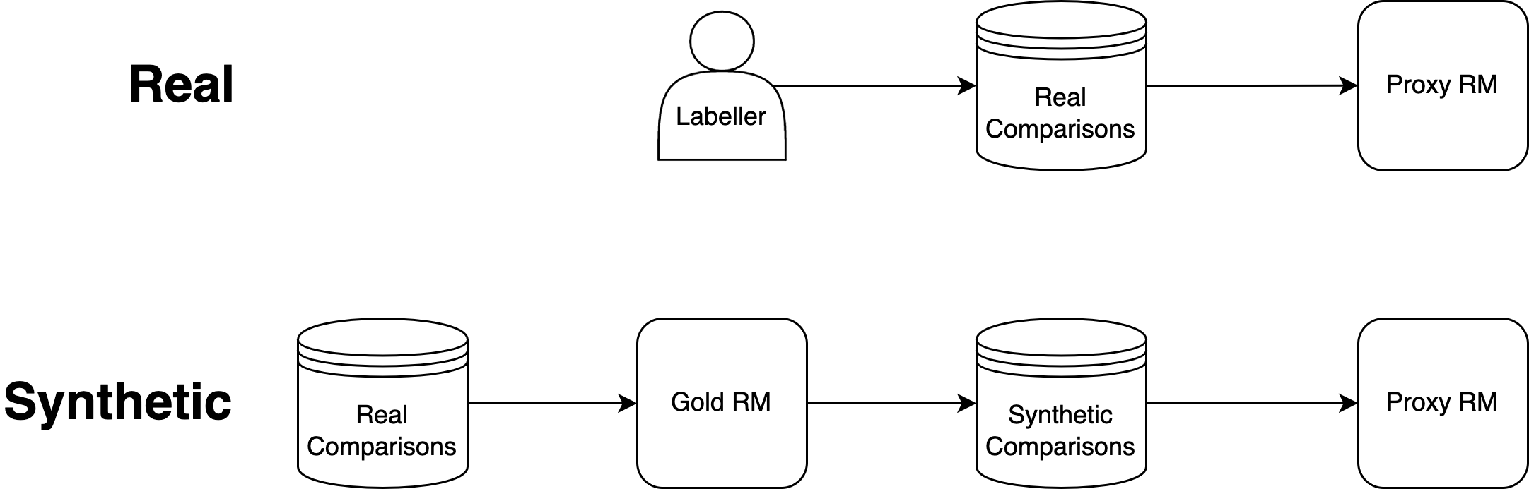
Because getting a ground truth gold reward signal from human labellers is expensive, we instead use a synthetic task where the ground truth is defined to be the output of a particular large "gold" RM. The 6B reward model from [4] is used as the gold RM, and our proxy RMs vary from 3M to 3B parameters[^5]. This synthetic gold reward is used to label pairs of rollouts from the policy given the same prompt to create synthetic RM training data. The synthetic comparisons are created deterministically by always marking the trajectory with the higher gold RM score as preferred.[^6] We generate 100, 000 synthetic comparisons and reserve 10% of these as a held out test set for computing the validation loss of RMs.

[^5]: We originally trained two additional RMs smaller than 3M parameters, which achieved near-chance accuracy and were off-trend, and so were excluded.

[^6]: We had experimented with sampling for creating labels, but observed noisier results.

See Figure 2 for a diagram of the synthetic setup.

2.2 Recalibration

The RM scores are translation-invariant, so to ensure comparability across different reward models, we recenter each RM such that the average reward of the initial policy is 0. We also unit normalize the variance of the gold RM scores.[^7] Because our hard thresholding synthetic data setup produces labels that are miscalibrated (since they do not incorporate the gold RM's confidence), we recalibrate the proxy RMs by rescaling the logits to minimize cross-entropy loss using a validation set of soft labels. All renormalization and recalibration is applied after the experiments; this does not affect BoN at all, and likely has no impact on RL because Adam is loss scale invariant, though it is possible that there are slight differences due to algorithmic details.

[^7]: We later decided this was unnecessary but decided not to change it.

3. Results

Section Summary: The researchers experimented with reward models to understand how they scale in terms of parameter count, training data size, and policy size during best-of-N sampling and reinforcement learning tasks. They discovered smooth improvements in true performance scores with more parameters or data, enabling predictions of peak results, but proxy scores were harder to model and often underestimated at higher complexities, with a key data threshold of about 2,000 comparisons needed for meaningful gains. Larger policies benefited less from optimization against these models but showed no increased tendency to overoptimize.

3.1 Fitting and validating functional forms

We chose our functional forms through experimentation with all RM data and parameter scaling curves in the remainder of this paper.

The BoN functional form was hypothesized using data up to $n = 1000$. In order to validate the functional forms, we performed a BoN experiment with up to $n = 60, 000$ (KL $\approx$ 10 nats), after only having seen data up to $n = 1, 000$ (KL $\approx$ 6 nats). As this experiment was conducted after the functional form was hypothesized based on data up to 6 nats, this was a true advance prediction.

We also test extrapolation of the BoN and RL functional forms from low KLs to to unseen larger KLs; see Figure 26 for details.

We also attempted to model the proxy scores but were unable to obtain a satisfactory fit. For BoN, despite visual similarity, a linear fit ($d\alpha_{\text{bo}n}$) did not work well (Figure 20). The predictions for RL and BoN are not as easily modelled as the gold score predictions. We leave a better understanding of the proxy RM score behavior to future work.

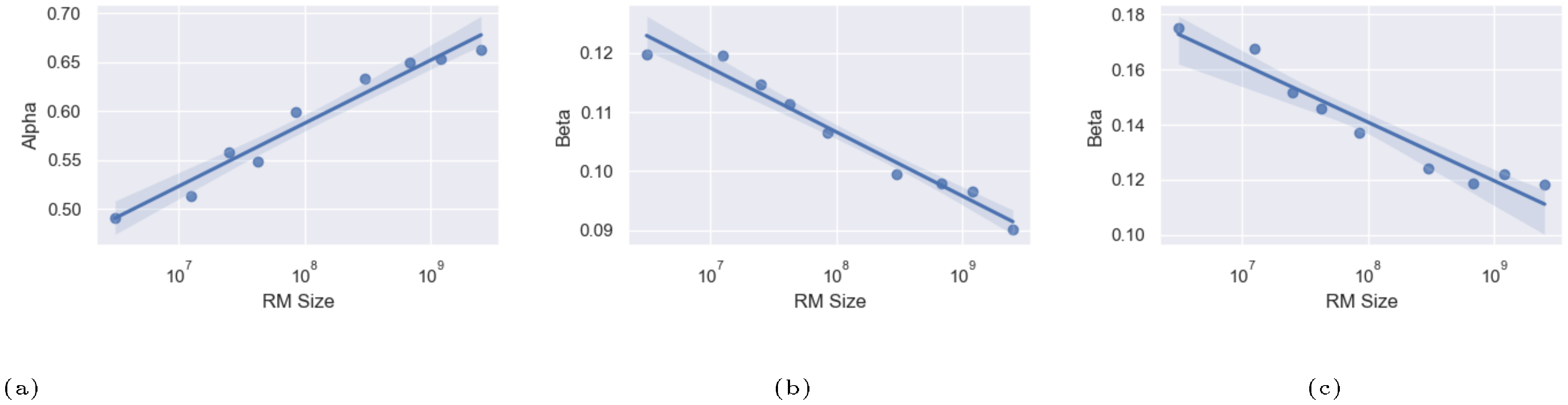
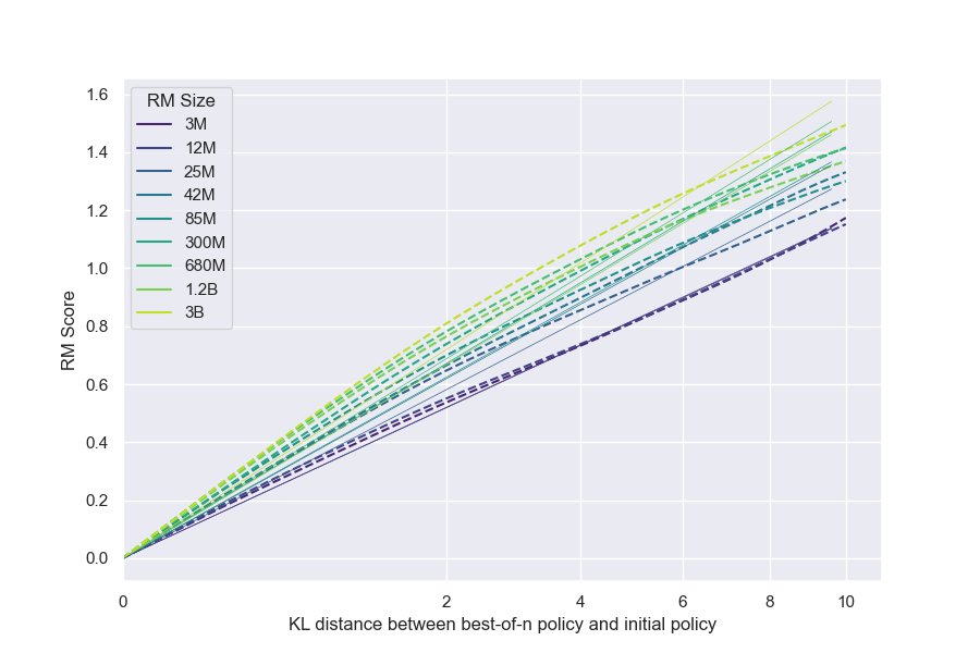
3.2 Scaling with RM Parameter Count

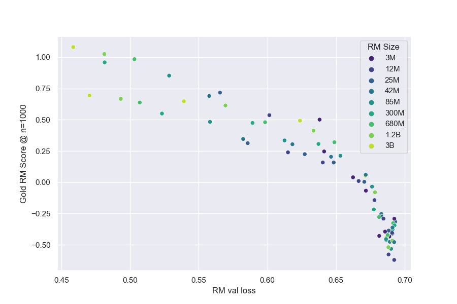
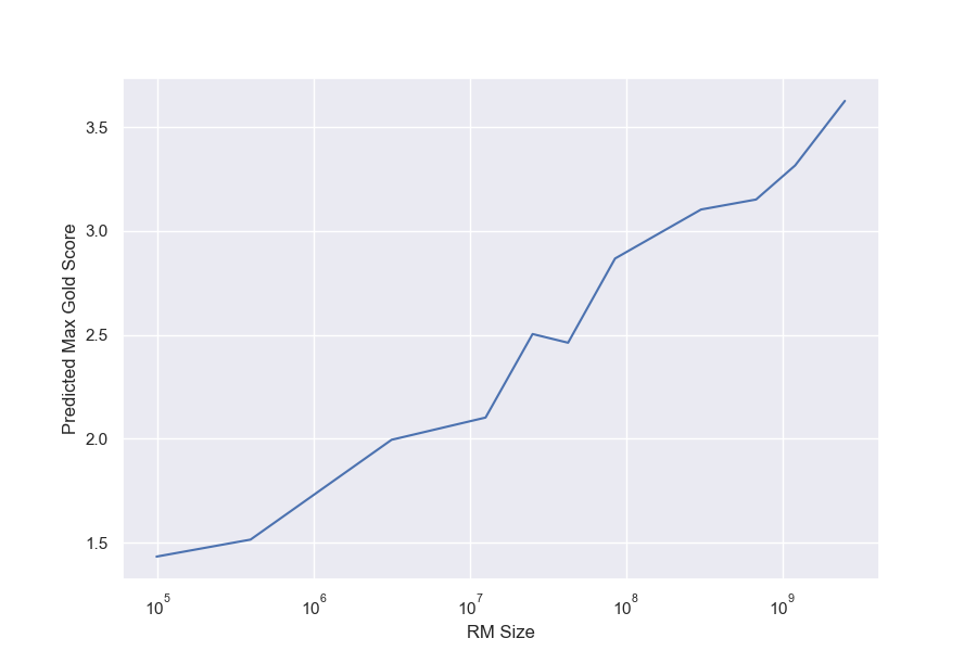
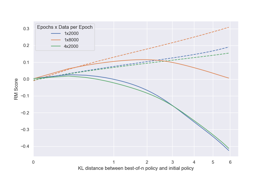
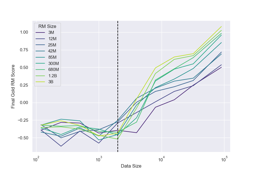
We hold policy size (1.2B) and data size (90, 000) constant (Figure 1). We observe that for the gold RM scores, $\alpha_{\text{bo}n}$ and $\beta_{\text{bo}n}$ change smoothly with RM size (Figure 3a and Figure 3b). For RL, we find that we can hold $\alpha_{\text{RL}}$ constant across all RM sizes, resulting in a clean scaling curve for $\beta_{RL}$ (Figure 3c). These scaling laws allow us to predict properties of training runs; for instance, we can also predict the peak gold RM scores for different RM sizes (Figure 12).

When modelled using the same functional forms as the respective gold scores, the proxy score fits have much lower values of $\beta_{\text{bo}n}$. We also see smooth scaling in the proxy score's $\alpha_{\text{bo}n}$ and $\beta_{\text{bo}n}$. However, for the reasons in Section 3.1, we are less confident about these fits. For both BoN and RL, we observe systematic underestimates of the proxy reward model when extrapolated to higher KLs. Both appear to eventually grow roughly linearly in $\sqrt{\text{KL}}$, as in [5].

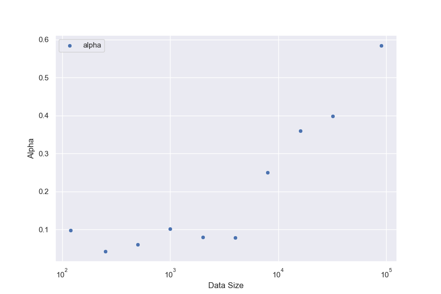
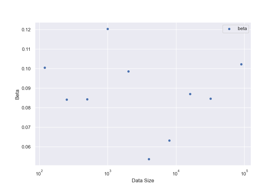
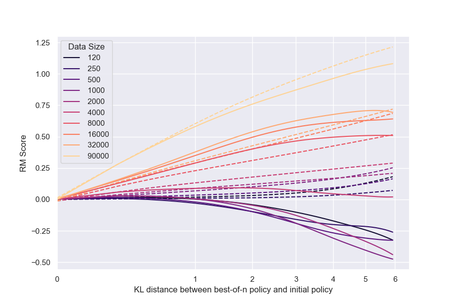
3.3 Scaling with RM Data Size

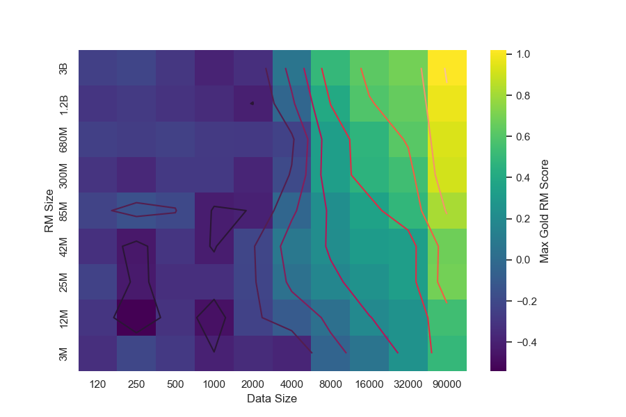
We hold RM size constant (12M) and sweep RM data size for both RL and BoN.[^8]. Overall, the results are consistent with intuition: more data leads to better gold scores and less goodharting. The scaling of $\alpha$ and $\beta$ with data size are not as cleanly described as for RM size scaling (Figure 17, Figure 18).

[^8]: For BoN, we actually sweep all combinations of RM size and data size; see Figure 10. For a version of Figure 4a against a 3B RM, see Figure 19.

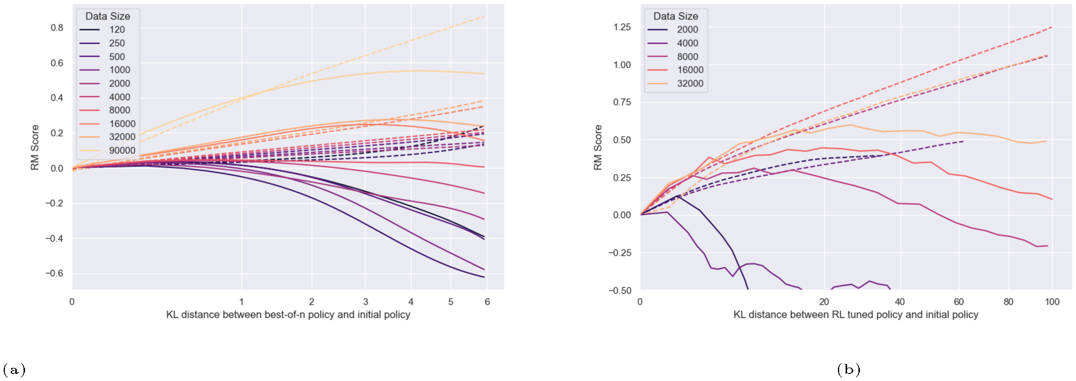
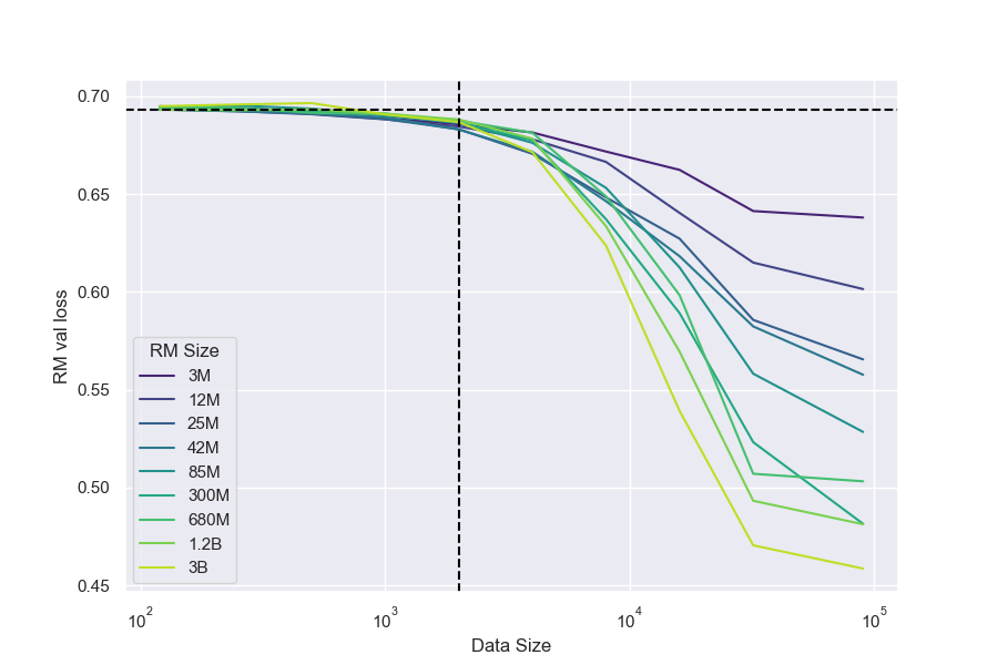
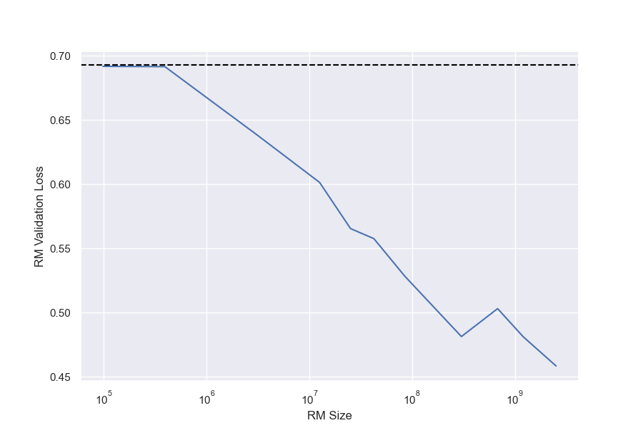
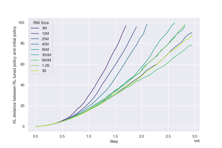
For all RM sizes, we observe that for amounts of data less than around 2, 000 comparisons[^9], there is very little improvement over near-chance loss (Figure 6). This is also reflected in gold scores after optimization (Figure 21). After this threshold, all models improve with more data, though larger RMs generally improve faster. Interestingly, although larger RMs result in better gold scores overall, they do not appear to have this critical threshold substantially earlier than smaller models.[^10]

[^9]: To test the hypothesis that some minimum number of RM finetuning steps is needed, we control for the number of SGD steps by running multiple epochs and observe that running 4 epochs instead of 1 yields no change in gold score whatsoever, whereas 1 epoch of 4 times as much data performs substantially better (Figure 13).

[^10]: This result contradicts some other internal findings; thus, it is possible that this is an artifact of this particular setup.

We hypothesized that two RMs of equal validation loss would achieve the same robustness against optimization, regardless of the combination of RM size and RM data size. Our results provide some weak evidence for this hypothesis (Figure 5).

3.4 Scaling with Policy Size

We briefly explore the impact of policy size by holding the RM size constant (12M) and evaluating two different policy sizes. We also perform the same experiment with a different RM size (3B), observing similar results (Figure 22).

Larger policies see less benefit from optimization against an RM, but don't overoptimize more.

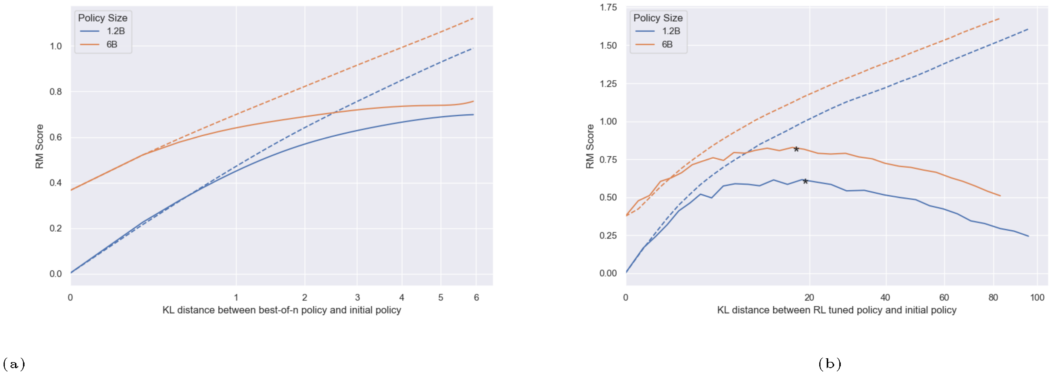
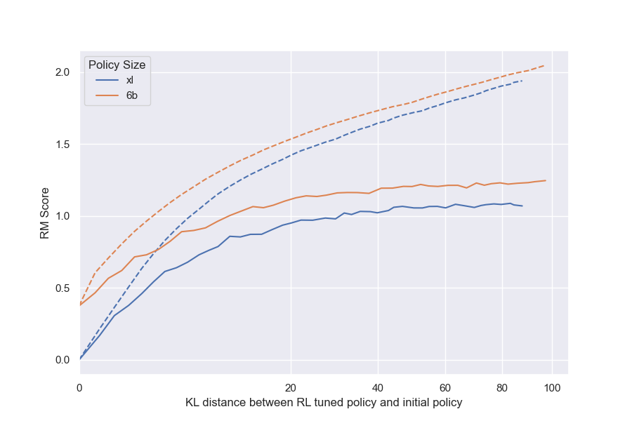
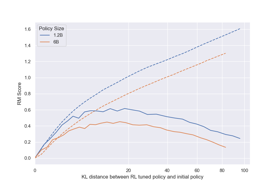
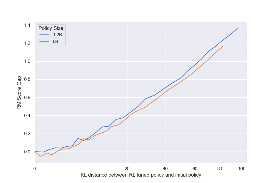
We observe that the 6B policy run has a smaller difference between its initial and peak gold reward model scores than the 1.2B policy run. This is most visible in the BoN plot (Figure 7a).[^11] However, while we might expect that a larger policy overoptimizes substantially faster, contrary to intuition, we find that both gold scores peak at almost the same KL. In fact, the gap between the proxy and gold scores is almost the same between the two policy sizes (Figure 24). We can interpret this gap, the shortfall between the predicted and actual rewards, as being indicative of the extent to which the proxy RM is exploited. We discuss this result further in Section 4.4.

[^11]: For a version of the RL plot (Figure 7b) with all runs starting at 0, see Figure 23.

3.5 RL vs BoN

A priori, we might expect reinforcement learning via PPO ([8]) and best-of-n to apply optimization in very different ways. As such, we ask whether this difference in optimization results in different overoptimization characteristics. Similarities would potentially indicate candidates for further study in gaining a more fundamental understanding of overoptimization in general, and differences opportunities for better optimization algorithms. We note the following:

RL is far less KL-efficient than BoN.

Viewing KL distance as a resource to be spent, we observe that RL "consumes" far more KL than BoN. This means that both optimization and overoptimization require more KL to occur with RL. Intuitively, BoN searches very locally around the initial policy, and thus $\text{KL}_{\text{bo}n}$ increases with roughly $\log(n)$. For RL on the other hand, each step modifies the policy from the policy of the previous step—KL increases approximately quadratically with step in the absence of KL penalty (Figure 16, Figure 14). An implication of this result is that KL distance is an inadequate metric for quantity of (over)optimization; we discuss this further in Section 4.1.

When looking at proxy vs gold RM scores, BoN and RL look more similar.

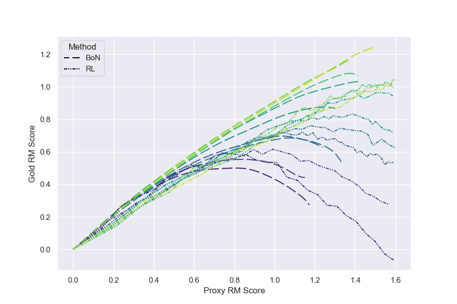
The proxy RM score is another possible metric for quantity of optimization, because it is the value that is being directly optimized for. Using it as the metric of optimization leads to significantly more analogy between RL and BoN than KL distance does. However, we do observe that RL initially has a larger proxy-gold gap (i.e requires more proxy RM increase to match BoN), but then peaks at a higher gold RM score than BoN (Figure 8).

3.6 Effect of KL Penalty

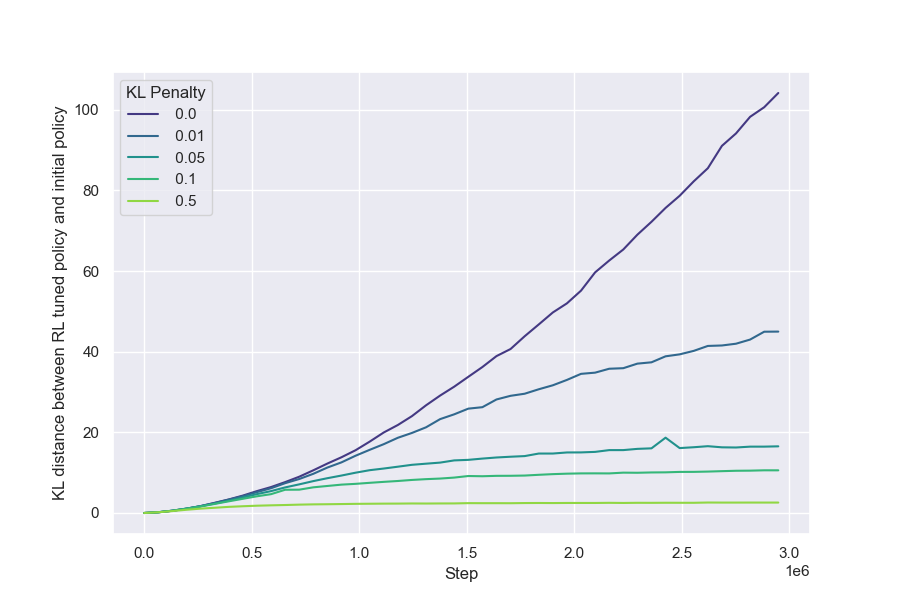
We observe in our setting that when varying the KL penalty for RL, the gold RM scores depend only on the KL distance of the policy $\text{KL}{\text{RL}}$ (Figure 9). The KL penalty only causes the gold RM score to converge earlier, but does not affect the $\text{KL}{\text{RL}}$-gold reward frontier, and so the effect of the penalty on the gold score is akin to early stopping (Figure 14). However, we have seen some evidence that this result could be particularly sensitive to hyperparameters.

Because we observe that using KL penalty has a strictly larger proxy-gold gap, we set KL penalty to 0 for all other RL experiments in this paper.

It is important to note that PPO's surrogate objective incorporates an implicit penalty on $D_{\text{KL}}\left(\pi_{\text{old}}\parallel\pi\right)$, where $\pi_{\text{old}}$ is a recent policy (not the initial policy) ([8]). This penalty is used to control how fast the policy changes, but also has an indirect effect on the KL we study here, $D_{\text{KL}}\left(\pi\parallel\pi_{\text{init}}\right)$, causing it to grow much more slowly (providing the implementation is well-tuned). We do not know why this indirect effect appears to lead to less overoptimization than an explicit KL penalty.

4. Discussion

Section Summary: The discussion explains that while Kullback-Leibler (KL) divergence provides a useful measure of optimization intensity for the same method, it falls short for comparing different algorithms because irrelevant changes can inflate KL without improving rewards. It frames the study's findings through Goodhart's Law, a concept about how proxies for measuring quality can backfire under optimization: regressional effects waste effort on noisy signals, extremal effects cause failures when behaviors shift outside the proxy's training range leading to non-monotonic performance drops, causal effects exploit false correlations, and adversarial effects—where the system tricks the proxy—aren't yet seen but could emerge later. These insights suggest that as reward models improve, they reduce over-optimization risks, with caution advised for future AI applications like iterated reinforcement learning from human feedback.

4.1 KL as a measure of amount of optimization

For any given fixed optimization method, KL yields clean scaling trends, such as the ones observed in Section 3.2, and consistent peak gold RM score KLs as in Figure 7. However, because it's clear that different methods of optimization spend KL very differently (Section 3.5), it should not be used to compare the amount of optimization between different optimization algorithms. There exist pertubations to a policy that are orthogonal to the reward signal that would result in increases in KL that do not increase either gold or proxy reward; conversely, extremely small but well targeted perturbations could substantially change the behavior of the policy within a small KL budget.

4.2 Relation to Goodhart Taxonomy

One useful taxonomy for various Goodhart effects is presented in [9], categorizing Goodhart's Law into 4 categories: Regressional, Extremal, Causal, and Adversarial. In this section, we discuss our results in the framework of this taxonomy.

4.2.1 Regressional Goodhart

Regressional Goodhart occurs when our proxy RMs depend on features with noise. The simplest toy example of this is a proxy reward $\hat{X}$ which is exactly equal to the gold reward $X$ plus some independent noise $Z$. When optimizing against this proxy, some amount of optimization power will go to selecting for noise, leading to a gold reward less than predicted by the proxy.

More formally, for independent absolutely continuous random variables $X$ and $Z$ with $X$ normally distributed and either (a) $Z$ normally distributed or (b) $\left|Z-\mathbb E\left[Z\right]\right|<\delta$ for some $\delta>0$, this model predicts a gold reward that is:

$ \mathbb E[X \mid \hat{X} = \hat{x}] = \mathbb E[X] + \left(\hat{x} - \mathbb E[X] - \mathbb E[Z]\right) \frac{\mathrm{Var}(X)}{\mathrm{Var}(X) + \mathrm{Var}(Z)}+\varepsilon\tag{1} $

where $\varepsilon=0$ in case (a) and $\varepsilon=o\left(\mathrm{Var}\left(Z\right)\right)$ as $\delta\to 0$ in case (b). See Appendix A for the proof.

Intuitively, we can interpret Equation 1 as stating that the optimization power expended is divided between optimizing the gold reward and selecting on the noise proportional to their variances. This also implies that if this is the only kind of Goodhart present, the gold reward must always increase monotonically with the proxy reward; as we observe nonmonotonic behavior (Figure 8), there must be either noise distributions violating these assumptions or other kinds of Goodhart at play.

This result lends itself to an interpretation of the $\alpha$ term in the RL and BoN gold score scaling laws: since for both RL and BoN the proxy scores are roughly linear in $\sqrt{\text{KL}}$, the difference in the slope of the proxy score and the linear component of the gold score (i.e the $\alpha$ term) can be interpreted as the amount of regressional Goodhart occurring.

4.2.2 Extremal Goodhart

We can think of out of distribution failures of the RM as an instance of extremal Goodhart. As we optimize against the proxy RM, the distribution of our samples shifts out of the training distribution of the RM, and thus the relation between the proxy and gold scores weakens. For instance, suppose in the training distribution a feature like answer length always indicates a higher quality answer, and thus the proxy RM infers that longer answers are always better, even though at some point outside the training distribution, selecting on longer answers no longer improves quality.[^12]

[^12]: Optimized policies producing very long answers even when a short answer would be preferred is a real issue that we have observed in other experiments in the InstructGPT setting.

We can also think of this as the proxy failing to depend on relevant features; this failure bears resemblance to the setting considered in [10], where a failure of the proxy to consider all features, under certain conditions, leads to overoptimization with unbounded loss of utility regardless of optimization method.

We expect extremal Goodharting to be primarily responsible for the nonmonotonicity of the gold RM scores in this paper, and is mostly responsible for the $\beta$ term, which in the limit of optimization, results in an unbounded loss of utility. This lends a natural interpretation to the smooth decrease in $\beta$ for both BoN and RL with increased RM size as smooth improvements in model robustness (Figure 3).

4.2.3 Causal Goodhart

We can think of causal Goodhart as being a generalization of regressional Goodhart: there may exist correlations between features and gold score where the causal structure of the problem is such that selecting on the feature does not increase the gold score. For instance, suppose answer length is correlated with quality due to some other common cause (say, informativeness); then, the proxy RM may learn to use answer length as a feature, and when we select against the proxy we get longer answers that do not increase on actual quality.[^13] In our experiments, we would observe causal Goodhart as behaving similarly to regressional Goodhart.

[^13]: We can think of noise as a particular case of this where the independent noise is correlated with signal+noise, but of course there is no causal relation between signal and noise.

4.2.4 Adversarial Goodhart

Adversarial Goodhart occurs when the policy actively manipulates the proxy. We do not expect the effects of adversarial Goodhart to be captured in this work, as the models involved are not powerful enough to implement adversarial strategies. However, given the constant improvement of ML capabilities, it is entirely plausible that ML systems will one day become capable enough to do so ([11]). When this occurs, the scaling laws observed in this paper may break down. Thus, we advise caution when using these results for extrapolation.

4.3 Implications for iterated RLHF

When conducting reinforcement learning from human feedback, it is preferable to use an online setup, in which fresh human feedback data is periodically used to train a new reward model, to mitigate overoptimization ([5]). Our scaling law allows us to analyze the effect of this iterative approach under some simplifying assumptions. We assume firstly that the scaling coefficients $\alpha_{\text{RL}}$ and $\beta_{\text{RL}}$ remain constant across iterations, and secondly that the distance $d=\sqrt{\text{KL}}$ is additive across iterations (because of how KL appears to grow empirically as in Figure 14). Under these assumptions, the final gold reward model score after $k$ iterations each covering a distance $d/k$ is given by

$ R_{\text{RL}}\left(d\right) = d\left(\alpha_{\text{RL}}-\beta_{\text{RL}}\log\left(d\right)+\beta_{\text{RL}}\log\left(k\right)\right). $

Two interesting observations follow from this. Firstly, the iterative approach does not affect any Goodharting captured by the $\alpha_{\text{RL}}$ term (such as regressional Goodharting, as discussed in Section 4.2.1). Secondly, the effect of the iterative approach is to increase the final gold RM score by an amount proportional to both $d$ and $\log\left(k\right)$, namely

$ \beta_{\text{RL}}d\log\left(k\right). $

Note that this result can only hold up to some maximum value of $k$, and we expect our scaling law to break down below some minimum distance. Further research is required to determine what this minimum is, as well as to what extent our simplifying assumptions hold in practice.

4.4 Policy size independence

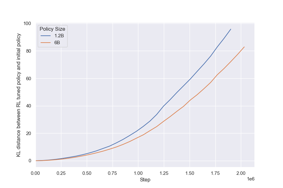
Our observation that larger SFT policies seem to exhibit the same amount of overoptimization during RL implies that larger policies do not increase the amount of optimization power applied to the RM or learn faster, even though they start out with higher performance on the gold score. While it is expected that larger policies have less to gain from optimizing against the same RM, we might also expect the gold score to peak at a substantially earlier KL distance, analogous to what we see when we scale the RM size (Section 3.2), or for larger policies to more efficiently utilize the same number of RL feedback steps (Section 3.3)[^14].

[^14]: It is also not the case that the 6B policy run has higher KL distance for the same number of RL steps; in fact, we observe that it has lower KL distance for the same number of steps (Figure 15)

One possible hypothesis is that, because RLHF can be viewed as Bayesian inference from the prior of the initial policy ([12])[^15], increases in policy size are only improving the modelling accuracy of the human demonstration distribution.

[^15]: The result of [12] concerns varying KL penalties rather than KL distances with no KL penalty, but as we observe in Section 3.6, this is equivalent on our setting.

4.5 Limitations and Future Work

In addition to the overoptimization studied in this paper (due to the mismatch between the reward model and the ground truth labels), there exists another source of overoptimization due to mismatch between the ground truth labels and the actual human intent. This contains issues ranging from the mundane, such as labellers choosing options that only appear to match their intent[^16], to substantially more philosophically fraught issues ([13, 14]). The main limitation of this work is that this additional source of overoptimization is not captured in the setting of this paper. See Section 5 for discussion of related work in alignment.

[^16]: For instance, the example of a robotic hand learning from human feedback to only appear to grasp a ball, presented in https://openai.com/blog/deep-reinforcement-learning-from-human-preferences/ ([15])

Some additional limitations and future directions include:

• Validating these results on other environments and experimental setups. While the experiments in this paper all use the InstructGPT environment, the main value of these results lies in the extent to which they reflect general phenomema. Confirming whether these results generalize to other settings would be extremely valuable to that end.[^2]
• Validating the synthetic setting. The synthetic setting might not transfer to real world settings, for instance because there is substantial correlation between RMs.
• Investigating methods for making RMs more robust to optimization. While there has been prior work in this direction (see Section 5), there is still much work to be done in systematically investigating ways to make RMs more robust.
• Exploring other forms of optimization and categorizing their differences. While this work focuses exclusively on BoN and RL there are other ways of applying optimization pressure against a model of a reward signal, either implicit or explicit. This includes GeDi-like steering, Decision Transformers[^3], variants of BoN like beam search, and other RL algorithms.
• Better understanding the functional form of proxy RM scores. In our modeling, we find that the proxy RM scores are more difficult to predict for both BoN and RL (Section 3.2). While they seem to have a major linear component, there is sufficient variation that fitting a linear regression is not very good at predicting extrapolated proxy RM scores.
• Exploring adversarial Goodhart empirically. In this work we deal with systems not powerful enough to cause adversarial Goodhart. However, it is plausible that adversarial Goodhart is especially important, or is associated with phase changes that break the trends seen in this paper.
• Exploring scaling with policy size in more detail. Our exploration of policy size scaling in this paper was limited to only two policy sizes. It is possible that there exist trends not seen in our exploration when considering the policy size more carefully.
• Exploring multi-iteration RLHF. In particular, checking for deviations from the assumptions of Section 4.3.

[^2]: In the course of our experiments, we observed visually similar results on the WebGPT environment ([2]).

[^3]: One could consider measuring the actual achieved ground truth/gold score achieved for each "proxy" score conditioned on, a la Figure 8, as testing the implicit reward-behavior mapping encoded by the model.

We hope this paper leads to future work further bridging conceptual and empirical alignment research.

5. Related Work

Section Summary: This section reviews the origins and applications of Goodhart's Law, a principle noting how optimizing a proxy measure can lead to unintended results, with early formulations from the 1970s and recent studies exploring overoptimization in reward models, often called reward hacking, including examples in reinforcement learning environments and theoretical models showing sudden shifts in performance. It also connects this to overfitting in machine learning, where models perform well on training data but fail to generalize, and to adversarial attacks that exploit vulnerabilities in neural networks, alongside scaling laws that predict model behavior as they grow larger. Finally, it discusses reinforcement learning from human feedback as a tool for aligning language models with human goals, while highlighting broader AI alignment challenges and the risks of misalignment in advanced systems leading to potential catastrophes.

Goodhart's Law in its modern formulation was first introduced in [16], with many of the key ideas introduced in prior works ([17, 18]). Many approaches have been proposed for reducing overoptimization in general ([19, 20]), as well as in RMs ([21]), including within the field of adversarial robustness ([22]). Overoptimization of reward models can be viewed as a special case of specification gaming (also known as reward hacking). Previous work has shown numerous examples of such behavior in a wide variety of settings ([23, 24]). [25] explores a diverse set of RL environments and finds phase transitions in some settings. A number of works have proposed theoretical models of Goodhart's Law and reward hacking ([26, 9, 27]), including [10] which exhibits very similar overoptimization curves as observed in this paper in some toy environments.

One can think of overfitting as a special case of Goodhart's law where the proxy is the score on some finite set of samples, whereas our actual objective includes its generalization properties as well. Overfitting has been observed and studied in RL settings ([28, 29, 30, 31]). [32] studies "observational overfitting" in RL settings, which is closely related to causal Goodhart ([9]).

Adversarial attacks and robustness are also very closely related fields. Many works have demonstrated the existence of adversarial examples in all kinds of neural networks ([33, 34, 35, 36]), and proposed methods to measure and increase neural network robustness ([37, 38, 39, 40]).

Scaling laws have seen substantial success in machine learning for predicting properties of language models ([41, 42, 43]) and has led to better theoretical understanding of language models ([44, 45]).

Reinforcement learning from human feedback ([15, 46]) has been used broadly in language models ([1, 4, 2, 5]). It is also a first step towards recursive reward modelling ([47]), an approach towards reducing the additional source of overoptimization described in Section 4.5, though it is subject to some theoretical limitations ([48]). We observe similar approximately-linear proxy RM scores observed in [5][^17], though we observe an early-KL bend in the proxy RM scores, and there are some occasional outliers with very small RMs and data sizes.

[^17]: Note that [5] scaled the policy size with the RM size, while we hold the policy size constant.

More broadly, AI alignment is the problem of ensuring that the goals of AI systems are aligned with the goals of humans ([49]), including future AI systems which may exceed humans ([50]). There are a number of reasons to expect AI misalignment, especially in those more powerful future systems, to occur ([51, 52, 53, 11, 54]), and to result in catastrophic outcomes ([55, 56]).

Acknowlegements

We thank Vivek Hebbar, Jared Kaplan, Jan Leike, Kyle McDonell, Dan Mossing, Ethan Perez, Laria Reynolds, and Jeff Wu for valuable discussion and feedback.

Appendix

Section Summary: The appendix begins with a mathematical proof for a lemma on the expected value of one random variable given the sum with another, focusing on cases where the variables are normally distributed or nearly constant, which supports an identity related to regression errors. It then explores alternative formulations for reinforcement learning models to ensure smooth behavior at low optimization levels, testing logarithmic and power-law options while noting trade-offs in fit and complexity. Finally, it lists key hyperparameters for the experiments, such as learning rates and batch sizes, and includes figures showing how model and data sizes influence performance scores, losses, and divergence measures in AI training setups.

A. Proof of Regressional Goodhart identity

########## {caption="Lemma"}

Let $X$ and $Z$ be independent absolutely continuous random variables with $X$ normally distributed and either (a) $Z$ normally distributed or (b) $\left|Z-\mathbb E\left[Z\right]\right|<\delta$ for some $\delta>0$. Then for any real number $c$ and as $\delta\to 0$,

$ \mathbb E\left[X\mid X+Z=c\right]=\mathbb E\left[X\right]+\left(c-\mathbb E\left[X\right]-\mathbb E\left[Z\right]\right)\frac{\mathrm{Var}\left(X\right)}{\mathrm{Var}\left(X\right)+\mathrm{Var}\left(Z\right)}+\varepsilon, $

where $\varepsilon=0$ in case (a) and $\varepsilon=o\left(\mathrm{Var}\left(Z\right)\right)$ in case (b).

Proof: First note that by making the substitutions $X^\prime=X-\mathbb E\left[X\right]$ and $Z^\prime=Z-\mathbb E\left[Z\right]$, we may assume without loss of generality that $\mathbb E\left[X\right]=\mathbb E\left[Z\right]=0$. Let $\mathrm{Var}\left(X\right)=\sigma^2$ and $\mathrm{Var}\left(Z\right)=\tau^2$.

In case (a), the pair $\left(X, X+Z\right)$ is bivariate normal with covariance matrix

$ \begin{pmatrix} \sigma^2 & \sigma^2\ \sigma^2 & \sigma^2+\tau^2 \end{pmatrix}, $

and the result follows by standard properties of conditional distributions of multivariate normal distributions.

In case (b), let $f_X$ and $f_Z$ be the probability density functions of $X$ and $Z$ respectively. Then

$ \begin{split} \mathbb E\left[X\mid X+Z=c\right]&=\frac{\int_{-\infty}^{\infty}\left(c-z\right)f_X\left(c-z\right)f_Z\left(z\right)\mathrm dz}{\int_{-\infty}^{\infty}f_X\left(c-z\right)f_Z\left(z\right)\mathrm dz}\ &=c-\frac{\int_{-\delta}^{\delta}z\left(f_X\left(c\right)-f^\prime_X\left(c\right)z+o\left(z\right)\right)f_Z\left(z\right)\mathrm dz}{\int_{-\delta}^{\delta}\left(f_X\left(c\right)-f^\prime_X\left(c\right)z+o\left(z\right)\right)f_Z\left(z\right)\mathrm dz}\ &=c-\frac{f_X\left(c\right)\mathbb E\left[Z\right]-f^\prime_X\left(c\right)\mathbb E\left[Z^2\right]+o\left(\mathbb E\left[Z^2\right]\right)}{f_X\left(c\right)-f^\prime_X\left(c\right)\mathbb E\left[Z\right]+o\left(1\right)}\ &=c+\frac{f^\prime_X\left(c\right)}{f_X\left(c\right)}\tau^2+o\left(\tau^2\right)\ &=c\left(1-\frac{\tau^2}{\sigma^2}\right)+o\left(\tau^2\right)\ &=c\left(\frac{\sigma^2}{\sigma^2+\tau^2}\right)+o\left(\tau^2\right), \end{split} $

as required.

B. RL form details

Ideally all overoptimization forms would have finite slope at the origin. We tried the following forms:

• ${d}\left(\alpha_{\text{RL}}-\beta_{\text{RL}}\log\left(1 + d\right)\right)$: Has slope $\alpha$ at the origin; however, has substantially worse extrapolation behavior. We can replace the 1 with a learned $\epsilon$ but that introduces another degree of freedom.
• Power laws ${d}\left(\alpha_{\text{RL}}-\beta_{\text{RL}}d^{\gamma_{\text{RL}}}\right)$: Has slope $\alpha$ at the origin; however, this adds another degree of freedom, and the best fits resulted in small values of $\gamma_{\text{RL}}$.

Note that the power law forms with small $\gamma_{\text{RL}}$ approximate the RL form that we decided on, as $\lim_{n \to \infty} n(x^{1/n} - 1) = \log x$.

C. Hyperparameters

: Table 1: Hyperparameters used throughout the experiments.

Hyperparameter	Value
RM Adam learning rate multiplier	1.67e-2
RM batch size	64
RL Adam learning rate multiplier	4e-3
RL batch size	256
RL PPO clipping parameter	0.2
RL Timesteps per rollout	256
RL minibatches per epoch	128
RL GAE bootstrapping parameter	0.95

: Table 2: A sample of the BoN answers on a single InstructGPT question (policy=1.2B, proxy RM=12M). For each individual question, the gold scores do not follow as clean a trend as they do when averaged over many questions as in Figure 1.

$n$	Generation	Proxy score	Gold score
1	Crime Mussels are typically found to be full of holes but will the moisture still be retained and will it hurt my eyes? The general response is yes as the clam is generally of a moistest nature. However, it all depends on the type of clam you are purchasing.<|endoftext|>	-0.1922	-0.5225
3	Most likely a pipe is having trouble staying full.<|endoftext|>	0.0322	-0.0165
10	A sponge<|endoftext|>	0.2336	0.4828
30	When something is full of holes, it is used for stirring or moving liquid.<|endoftext|>	0.6534	-0.1543
100	A tornado is usually a swirling cloud of swirling air with a spinning jet which stirs up winds full of sharp debris.<|endoftext|>	0.8968	-0.3367
300	A tornado is usually a swirling cloud of swirling air with a spinning jet which stirs up winds full of sharp debris.<|endoftext|>	0.8968	-0.3367
1000	A tornado is usually a swirling cloud of swirling air with a spinning jet which stirs up winds full of sharp debris.<|endoftext|>	0.8968	-0.3367
3000	A bore hole is a hole drilled into a rock for the purpose of exploring a fossil-bearing sedimentary or bedrock deposit.<|endoftext|>	0.9003	0.2733
10000	A bore hole is a hole drilled into a rock for the purpose of exploring a fossil-bearing sedimentary or bedrock deposit.<|endoftext|>	0.9003	0.2733
30000	A pothole is a structural vulnerability that allows water to penetrate its cavity and cause damage to passing vehicles or the surface it rests on.<|endoftext|>	0.9527	0.5490

References

[1] Nisan Stiennon et al. (2020). Learning to summarize from human feedback. Computing Research Repository. arXiv:2009.01325v3.

[2] Nakano et al. (2021). WebGPT: Browser-assisted question-answering with human feedback. arXiv preprint arXiv:2112.09332.

[3] Menick et al. (2022). Teaching language models to support answers with verified quotes. arXiv preprint arXiv:2203.11147.

[4] Long Ouyang et al. (2022). Training language models to follow instructions with human feedback. version 1. arXiv:2203.02155v1.

[5] Bai et al. (2022). Training a Helpful and Harmless Assistant with Reinforcement Learning from Human Feedback. arXiv preprint arXiv:2204.05862.

[6] Glaese et al. (2022). Improving alignment of dialogue agents via targeted human judgements. https://storage.googleapis.com/deepmind-media/DeepMind.com/Authors-Notes/sparrow/sparrow-final.pdf.

[7] Brown et al. (2020). Language models are few-shot learners. arXiv preprint arXiv:2005.14165.

[8] Schulman et al. (2017). Proximal policy optimization algorithms. arXiv preprint arXiv:1707.06347.

[9] Manheim, David and Garrabrant, Scott (2018). Categorizing variants of Goodhart's Law. arXiv preprint arXiv:1803.04585.

[10] Zhuang, Simon and Hadfield-Menell, Dylan (2020). Consequences of misaligned AI. Advances in Neural Information Processing Systems. 33. pp. 15763–15773.

[11] Hubinger et al. (2019). Risks from learned optimization in advanced machine learning systems. arXiv preprint arXiv:1906.01820.

[12] Korbak et al. (2022). RL with KL penalties is better viewed as Bayesian inference. arXiv preprint arXiv:2205.11275.

[13] Armstrong, Stuart and Mindermann, Sören (2018). Occam' s razor is insufficient to infer the preferences of irrational agents. In Advances in Neural Information Processing Systems. pp. . https://proceedings.neurips.cc/paper/2018/file/d89a66c7c80a29b1bdbab0f2a1a94af8-Paper.pdf.

[14] Sunstein et al. (2001). Predictably incoherent judgments. Stan. L. Rev.. 54. pp. 1153.

[15] Christiano et al. (2017). Deep reinforcement learning from human preferences. Advances in neural information processing systems. 30.

[16] Hoskin, Keith (1996). The "awful idea of accountability" : inscribing people into the measurement of objects. Accountability : power, ethos and the technologies of managing / edited by Rolland Munro and Jan Mouritsen.

[17] Campbell, Donald T (1969). Reforms as experiments.. American psychologist. 24(4). pp. 409.

[18] Goodhart, Charles (1975). Problems of monetary management: the UK experience in papers in monetary economics. Monetary Economics. 1.

[19] Taylor, Jessica (2016). Quantilizers: A safer alternative to maximizers for limited optimization. In Workshops at the Thirtieth AAAI Conference on Artificial Intelligence.

[20] Everitt et al. (2017). Reinforcement learning with a corrupted reward channel. arXiv preprint arXiv:1705.08417.

[21] Gleave, Adam and Irving, Geoffrey (2022). Uncertainty Estimation for Language Reward Models. arXiv preprint arXiv:2203.07472.

[22] Chakraborty et al. (2018). Adversarial attacks and defences: A survey. arXiv preprint arXiv:1810.00069.

[23] Victoria Krakovna et al. (2020). Specification gaming: the flip side of AI ingenuity. https://www.deepmind.com/blog/specification-gaming-the-flip-side-of-ai-ingenuity.

[24] Lehman et al. (2020). The surprising creativity of digital evolution: A collection of anecdotes from the evolutionary computation and artificial life research communities. Artificial life. 26(2). pp. 274–306.

[25] Pan et al. (2022). The effects of reward misspecification: Mapping and mitigating misaligned models. arXiv preprint arXiv:2201.03544.

[26] Victoria Krakovna and Ramana Kumar (2019). Classifying specification problems as variants of Goodhart’s Law. https://vkrakovna.wordpress.com/2019/08/19/classifying-specification-problems-as-variants-of-goodharts-law/.

[27] Skalse et al. (2022). Defining and Characterizing Reward Hacking. doi:10.48550/ARXIV.2209.13085. https://arxiv.org/abs/2209.13085.

[28] Zhang et al. (2018). A dissection of overfitting and generalization in continuous reinforcement learning. arXiv preprint arXiv:1806.07937.

[29] Zhang et al. (2018). A study on overfitting in deep reinforcement learning. arXiv preprint arXiv:1804.06893.

[30] Farebrother et al. (2018). Generalization and regularization in DQN. arXiv preprint arXiv:1810.00123.

[31] Cobbe et al. (2019). Quantifying Generalization in Reinforcement Learning. In Proceedings of the 36th International Conference on Machine Learning. pp. 1282–1289. https://proceedings.mlr.press/v97/cobbe19a.html.

[32] Song et al. (2019). Observational overfitting in reinforcement learning. arXiv preprint arXiv:1912.02975.

[33] Szegedy et al. (2013). Intriguing properties of neural networks. arXiv preprint arXiv:1312.6199.

[34] Lin et al. (2017). Tactics of Adversarial Attack on Deep Reinforcement Learning Agents. doi:10.48550/ARXIV.1703.06748. https://arxiv.org/abs/1703.06748.

[35] Ebrahimi et al. (2018). On adversarial examples for character-level neural machine translation. arXiv preprint arXiv:1806.09030.

[36] Dai et al. (2018). Adversarial Attack on Graph Structured Data. In Proceedings of the 35th International Conference on Machine Learning. pp. 1115–1124. https://proceedings.mlr.press/v80/dai18b.html.

[37] Gu, Shixiang and Rigazio, Luca (2014). Towards deep neural network architectures robust to adversarial examples. arXiv preprint arXiv:1412.5068.

[38] Zheng et al. (2016). Improving the robustness of deep neural networks via stability training. In Proceedings of the ieee conference on computer vision and pattern recognition. pp. 4480–4488.

[39] Carlini et al. (2019). On Evaluating Adversarial Robustness. doi:10.48550/ARXIV.1902.06705. https://arxiv.org/abs/1902.06705.

[40] Guo et al. (2021). Gradient-based Adversarial Attacks against Text Transformers. doi:10.48550/ARXIV.2104.13733. https://arxiv.org/abs/2104.13733.

[41] Kaplan et al. (2020). Scaling laws for neural language models. arXiv preprint arXiv:2001.08361.

[42] Henighan et al. (2020). Scaling laws for autoregressive generative modeling. arXiv preprint arXiv:2010.14701.

[43] Hernandez et al. (2021). Scaling laws for transfer. arXiv preprint arXiv:2102.01293.

[44] Sharma, Utkarsh and Kaplan, Jared (2020). A neural scaling law from the dimension of the data manifold. arXiv preprint arXiv:2004.10802.

[45] Bahri et al. (2021). Explaining neural scaling laws. arXiv preprint arXiv:2102.06701.

[46] Ibarz et al. (2018). Reward learning from human preferences and demonstrations in atari. Advances in neural information processing systems. 31.

[47] Leike et al. (2018). Scalable agent alignment via reward modeling: a research direction. arXiv preprint arXiv:1811.07871.

[48] Paul Christiano et al. (2021). Eliciting latent knowledge: How to tell if your eyes deceive you. https://docs.google.com/document/d/1WwsnJQstPq91_Yh-Ch2XRL8H_EpsnjrC1dwZXR37PC8.

[49] Ngo, Richard (2022). The alignment problem from a deep learning perspective. arXiv preprint arXiv:2209.00626.

[50] Bostrom, Nick (2014). Superintelligence: Paths, Dangers, Strategies. Oxford University Press, Inc..

[51] Stephen M. Omohundro (2008). The Basic AI Drives. In Proceedings of the First Conference on Artificial General Intelligence. pp. 483–492. http://selfawaresystems.files.wordpress.com/2008/01/ai_drives_final.pdf.

[52] Turner et al. (2021). Optimal Policies Tend To Seek Power. In Advances in Neural Information Processing Systems. pp. 23063–23074. https://proceedings.neurips.cc/paper/2021/file/c26820b8a4c1b3c2aa868d6d57e14a79-Paper.pdf.

[53] Armstrong, Stuart and others (2013). General purpose intelligence: arguing the orthogonality thesis. Analysis and Metaphysics. 12(68). pp. 1–20.

[54] Soares et al. (2015). Corrigibility. In Workshops at the Twenty-Ninth AAAI Conference on Artificial Intelligence.

[55] Carlsmith, Joseph (2022). Is Power-Seeking AI an Existential Risk?. arXiv preprint arXiv:2206.13353.

[56] Ajeya Cotra (2022). Without specific countermeasures, the easiest path to transformative AI likely leads to AI takeover. https://www.alignmentforum.org/posts/pRkFkzwKZ2zfa3R6H/without-specific-countermeasures-the-easiest-path-to.