Autoencoding beyond pixels using a learned similarity metric

Anders Boesen Lindbo LarsenSøren Kaae SønderbyHugo LarochelleOle Winther

article2015ICML2,263 citations

Proposes combining variational autoencoders and generative adversarial networks to measure reconstruction loss using learned discriminator features rather than pixel-wise comparisons, producing sharper images and enabling semantic latent vector arithmetic.

Listen

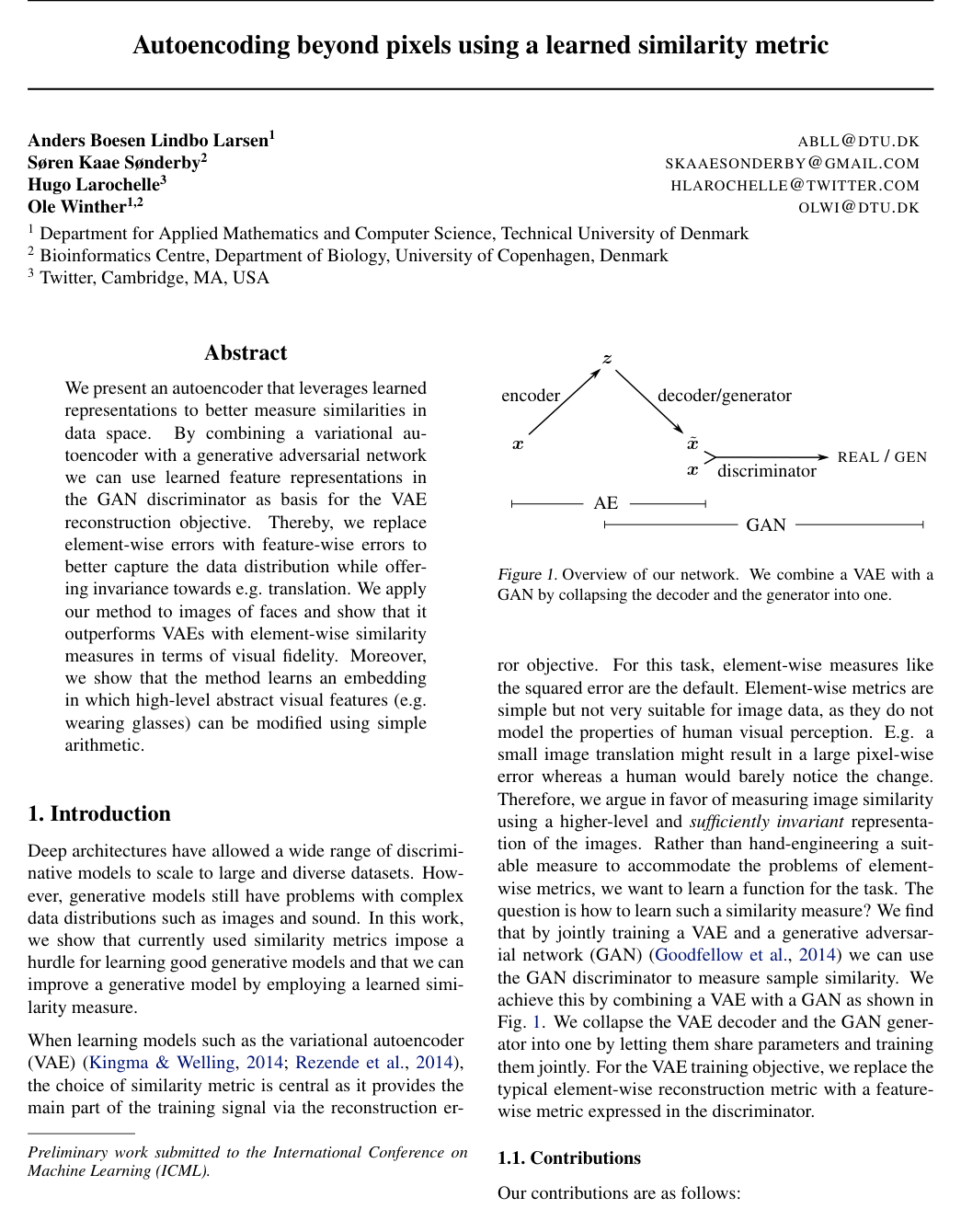
Generating realistic, high-dimensional visual data remains a central challenge in machine learning. Standard generative models, particularly variational autoencoders, typically rely on simple pixel-by-pixel distance metrics to measure reconstruction quality. These element-wise measures fail to align with human visual perception because minor spatial shifts cause large numerical penalties, frequently producing overly blurry reconstructions. The article sets out to demonstrate that combining a variational autoencoder with a generative adversarial network creates a hybrid architecture that learns high-level similarity metrics directly from data, significantly improving image quality and latent representation.

To evaluate this framework, the authors collapsed the decoder of the variational autoencoder and the generator of the generative adversarial network into a single shared network. Instead of comparing individual pixels, the model uses intermediate feature representations from the adversarial discriminator to measure reconstruction error while simultaneously training against adversarial objectives. The approach was tested unsupervised on benchmark datasets of 64x64 pixel face images, including the CelebA dataset containing 202,599 images and the Labeled Faces in the Wild dataset, without relying on manual metric engineering.

The findings show that the proposed hybrid model generates sharper, more natural face images and reconstructions compared to standard variational autoencoders, avoiding the off-center blurriness common in pixel-based methods. In quantitative attribute generation tests, the hybrid achieved a lower mean squared error of 22.39 compared to 27.59 for the standard variational autoencoder and 27.89 for a standalone generative adversarial network, as well as a higher cosine similarity score of 0.9114. Furthermore, the unsupervised training successfully disentangled visual concepts in latent space, enabling deliberate image manipulation—such as adding eyeglasses or altering hairstyles—via simple vector arithmetic while preserving identity and texture consistency.

These results indicate that learned, feature-level similarity metrics effectively overcome the structural limitations of element-wise objectives in image synthesis. Unifying image encoding and adversarial generation eliminates the need for hand-engineered distance metrics and expands the capability of unsupervised models to discover actionable semantic controls from unlabeled data. However, the model did not achieve state-of-the-art results when applied to semi-supervised classification on complex, high-variance datasets, and traditional pixel log-likelihood metrics deteriorated despite superior visual fidelity.

Organizations seeking to implement generative vision systems should consider adopting learned discriminator-based loss functions when visual quality and semantic manipulation are core priorities. Future work should explore using pretrained or specialized similarity networks and evaluate methods to stabilize training across broader, more diverse image categories before deploying this architecture to general object classification pipelines.

Technical University of Denmark Twitter University of Copenhagen gan generative adversarial networks reconstruction learned similarity metric variational autoencoder generative adversarial network

arXiv: 1512.09300 andersbll/autoencoding_beyond_pixels

Paper: Generative Adversarial Networks, Ian J. Goodfellow et al. (2014). This foundational paper introduces generative adversarial networks, providing the essential adversarial architecture and training mechanics that the source paper later combines with variational autoencoders.
Paper: Adversarial Autoencoders, Alireza Makhzani et al. (2015). This paper establishes the adversarial autoencoder framework, serving as a direct prerequisite for understanding the fusion of autoencoders and adversarial networks explored in the source.
Paper: Conditional Generative Adversarial Nets, Mehdi Mirza et al. (2014). This foundational work on conditional generative adversarial networks provides key architectural principles for conditioning generator networks that the source paper extends.

Paper: beta-VAE: Learning Basic Visual Concepts with a Constrained Variational Framework, Irina Higgins et al. (2016). This subsequent work builds directly on variational generative frameworks to explore disentangled latent representations, continuing the source's investigation into semantic image manipulation.
Paper: GIRAFFE: Representing Scenes as Compositional Generative Neural Feature Fields, Michael Niemeyer et al. (2021). This study extends the source's exploration of unsupervised latent space manipulation by introducing 3D-aware compositional neural fields for disentangled scene editing.
Paper: The Unreasonable Effectiveness of Deep Features as a Perceptual Metric, Richard Zhang et al. (2018). This research directly generalizes the source paper's core premise by demonstrating that deep network feature activations universally outperform traditional pixel metrics as perceptual similarity measures.

Cover for Autoencoding beyond pixels using a learned similarity metric

Abstract

We present an autoencoder that leverages learned representations to better measure similarities in data space. By combining a variational autoencoder with a generative adversarial network we can use learned feature representations in the GAN discriminator as basis for the VAE reconstruction objective. Thereby, we replace element-wise errors with feature-wise errors to better capture the data distribution while offering invariance towards e.g. translation. We apply our method to images of faces and show that it outperforms VAEs with element-wise similarity measures in terms of visual fidelity. Moreover, we show that the method learns an embedding in which high-level abstract visual features (e.g. wearing glasses) can be modified using simple arithmetic.

Topics

gan generative adversarial networks reconstruction variational autoencoders visual feature variational auto encoders semantic similarity

Keywords

1. Introduction
1.1. Contributions
2. Autoencoding with learned similarity
2.1. Variational autoencoder
2.2. Generative adversarial network
2.3. Beyond element-wise reconstruction error with VAE/GAN
3. Related work
4. Experiments
4.1. CelebA face images
4.1.1. VISUAL ATTRIBUTE VECTORS
4.2. Attribute similarity, Labeled faces in the wild
4.3. Unsupervised pretraining for supervised tasks
5. Discussion
Acknowledgements
References

Knowls

Knowl 1 — VAE/GAN Architecture Combining Variational Autoencoding with Adversarial Training
model/method
The VAE/GAN model integrates a Variational Autoencoder (VAE) and a Generative Adversarial Network (GAN) into a unified unsupervised generative framework. The architecture consists of three components:
1. An Encoder $\mathrm{Enc}(x)$ that maps a data sample $x$ to a latent distribution $q(z \mid x)$ .
2. A shared Decoder/Generator $\mathrm{Dec}(z)$ that maps a latent vector $z$ back to data space, simultaneously serving as the VAE decoder $p(x \mid z)$ and the GAN generator.
3. A Discriminator $\mathrm{Dis}(x)$ that outputs the probability that $x$ is a real data sample versus a generated sample, while also computing intermediate hidden feature representations $\mathrm{Dis}_l(x)$ at layer $l$ .
Instead of evaluating reconstruction error via element-wise pixel metrics (such as mean squared error), the model formulates the reconstruction loss in the feature space of the discriminator layer $\mathrm{Dis}_l$ . The objective function consists of three terms:

$\mathcal{L} = \mathcal{L}_{\mathrm{prior}} + \mathcal{L}_{\mathrm{llike}}^{\mathrm{Dis}_l} + \mathcal{L}_{\mathrm{GAN}}$

where $\mathcal{L}_{\mathrm{prior}} = D_{\mathrm{KL}}(q(z \mid x) \,\|\, p(z))$ regularizes the latent space towards prior $p(z) = \mathcal{N}(0, \mathbf{I})$ , $\mathcal{L}_{\mathrm{llike}}^{\mathrm{Dis}_l}$ measures feature-level reconstruction fidelity (content error), and $\mathcal{L}_{\mathrm{GAN}}$ encourages the generated images to lie on the data manifold (style/realism error).
Knowl 2 — Discriminator Feature-Space Reconstruction Loss
equation
Let $x$ be an input data sample, $z \sim q(z \mid x) = \mathrm{Enc}(x)$ be its latent encoding, and $\tilde{x} = \mathrm{Dec}(z)$ be the reconstructed sample. Let $\mathrm{Dis}_l(x)$ denote the hidden activation vector of the $l$ -th layer of the discriminator network $\mathrm{Dis}$ .

A Gaussian observation model is introduced on the feature representation $\mathrm{Dis}_l(x)$ with mean $\mathrm{Dis}_l(\tilde{x})$ and identity covariance matrix $\mathbf{I}$ :

$p(\mathrm{Dis}_l(x) \mid z) = \mathcal{N}\left(\mathrm{Dis}_l(x) \;\middle|\; \mathrm{Dis}_l(\tilde{x}),\, \mathbf{I}\right)$

The VAE reconstruction loss (expected negative log-likelihood) is then given by:

$\mathcal{L}_{\mathrm{llike}}^{\mathrm{Dis}_l} = -\mathbb{E}_{q(z \mid x)}\left[\log p(\mathrm{Dis}_l(x) \mid z)\right] = \frac{1}{2}\mathbb{E}_{q(z \mid x)}\left[\|\mathrm{Dis}_l(x) - \mathrm{Dis}_l(\mathrm{Dec}(z))\|_2^2\right] + \text{const}$

This replaces pixel-wise reconstruction errors with an abstract, high-level similarity metric learned by the discriminator, providing invariance to local image perturbations and spatial misalignments.
Knowl 3 — Adversarial Objective with Dual Negative Sampling
equation
In the VAE/GAN framework, the adversarial loss $\mathcal{L}_{\mathrm{GAN}}$ evaluates real data samples $x \sim p_{\mathrm{data}}(x)$ against two distinct sources of negative samples: prior-generated samples $\mathrm{Dec}(z_p)$ from $z_p \sim p(z) = \mathcal{N}(0, \mathbf{I})$ , and autoencoder reconstructions $\mathrm{Dec}(\mathrm{Enc}(x))$ from $z \sim q(z \mid x)$ :

$\mathcal{L}_{\mathrm{GAN}} = \log\big(\mathrm{Dis}(x)\big) + \log\big(1 - \mathrm{Dis}(\mathrm{Dec}(z_p))\big) + \log\big(1 - \mathrm{Dis}(\mathrm{Dec}(\mathrm{Enc}(x)))\big)$

where $\mathrm{Dis}(x) \in [0, 1]$ represents the probability that $x$ is an actual training sample. Including reconstructed samples $\mathrm{Dec}(\mathrm{Enc}(x))$ ensures that negative samples closely match specific positive examples $x$ in structure, supplying a more informative gradient signal to the discriminator and generator.
Knowl 4 — Joint VAE/GAN Training Algorithm and Parameter Update Routing
algorithm
Training VAE/GAN requires selectively routing gradient signals to specific subnetworks to avoid degenerate solutions (such as the discriminator collapsing its hidden representations to zero if updated by reconstruction loss):
Input: Dataset of samples, network parameters $\theta_{\text{Enc}}$ , $\theta_{\text{Dec}}$ , $\theta_{\text{Dis}}$ , weighting hyperparameter $\gamma > 0$
Output: Trained encoder, decoder/generator, and discriminator networks
repeat
    Sample mini-batch $X$ from dataset
     $Z \leftarrow \text{Enc}(X)$
     $\mathcal{L}_{\text{prior}} \leftarrow D_{\text{KL}}(q(Z|X) \,\|\, p(Z))$
     $\tilde{X} \leftarrow \text{Dec}(Z)$
     $\mathcal{L}_{\text{llike}}^{\text{Dis}_l} \leftarrow -\mathbb{E}_{q(Z|X)}[\log p(\text{Dis}_l(X)|Z)]$
    Sample $Z_p \sim \mathcal{N}(0, I)$
     $X_p \leftarrow \text{Dec}(Z_p)$
     $\mathcal{L}_{\text{GAN}} \leftarrow \log(\text{Dis}(X)) + \log(1 - \text{Dis}(\tilde{X})) + \log(1 - \text{Dis}(X_p))$
     $\theta_{\text{Enc}} \leftarrow \theta_{\text{Enc}} - \nabla_{\theta_{\text{Enc}}} (\mathcal{L}_{\text{prior}} + \mathcal{L}_{\text{llike}}^{\text{Dis}_l})$
     $\theta_{\text{Dec}} \leftarrow \theta_{\text{Dec}} - \nabla_{\theta_{\text{Dec}}} (\gamma \mathcal{L}_{\text{llike}}^{\text{Dis}_l} - \mathcal{L}_{\text{GAN}})$
     $\theta_{\text{Dis}} \leftarrow \theta_{\text{Dis}} - \nabla_{\theta_{\text{Dis}}} \mathcal{L}_{\text{GAN}}$
until convergence
The hyperparameter $\gamma > 0$ balances the decoder's reconstruction accuracy (content) against its ability to fool the discriminator (style). The adversarial loss $\mathcal{L}_{\mathrm{GAN}}$ is not backpropagated to $\theta_{\mathrm{Enc}}$ , and $\mathcal{L}_{\mathrm{llike}}^{\mathrm{Dis}_l}$ is not backpropagated to $\theta_{\mathrm{Dis}}$ . Training uses RMSProp with a learning rate of $0.0003$ and mini-batch size of 64. Layer $l$ in $\mathrm{Dis}$ is chosen after three spatial downsamplings by a factor of 2.
Knowl 5 — Latent Space Vector Arithmetic for Visual Attribute Modification
model/method
Unsupervised training of the VAE/GAN yields an aligned continuous latent space where semantic visual attributes can be manipulated via linear vector arithmetic. For any binary visual attribute $a$ , let $S_a^+$ denote the set of images possessing the attribute and $S_a^-$ denote the set of images lacking it. The visual attribute vector $v_a$ in the latent space is calculated as the difference between the mean latent representations:

$v_a = \frac{1}{|S_a^+|} \sum_{x \in S_a^+} \mathbb{E}_{q(z \mid x)}[z] - \frac{1}{|S_a^-|} \sum_{x \in S_a^-} \mathbb{E}_{q(z \mid x)}[z]$

To alter an input image $x$ with respect to attribute $a$ , the modified image $\tilde{x}_a$ is generated by shifting the latent encoding along $v_a$ :

$\tilde{x}_a = \mathrm{Dec}\left(\mathbb{E}_{q(z \mid x)}[z] + \alpha v_a\right)$

where $\alpha \in \mathbb{R}$ modulates the attribute intensity. This operation successfully adds or removes high-level attributes (e.g., eyeglasses, bangs, gray hair, mustache) while preserving unperturbed features such as subject identity and hair texture.
Knowl 6 — Convolutional Network Architectures for VAE/GAN
experimental setup
The standard network specifications for $64 \times 64 \times 3$ image processing across the three modules of VAE/GAN are defined as follows (where BNorm indicates batch normalization with per-channel normalization on convolutional layers, and stride 2 convolutions perform downsampling $\downarrow$ or upsampling $\uparrow$ via backward convolution/fractional striding):
- Encoder (Enc):
  - $5 \times 5$ conv, 64 channels, $\downarrow$ stride 2, BNorm, ReLU
  - $5 \times 5$ conv, 128 channels, $\downarrow$ stride 2, BNorm, ReLU
  - $5 \times 5$ conv, 256 channels, $\downarrow$ stride 2, BNorm, ReLU
  - Fully connected, 2048 units, BNorm, ReLU
  - Linear heads outputting mean and log-variance parameters for latent vector $z$
- Decoder/Generator (Dec):
  - Fully connected, $8 \times 8 \times 256$ units, BNorm, ReLU
  - $5 \times 5$ conv, 256 channels, $\uparrow$ stride 2, BNorm, ReLU
  - $5 \times 5$ conv, 128 channels, $\uparrow$ stride 2, BNorm, ReLU
  - $5 \times 5$ conv, 32 channels, $\uparrow$ stride 2, BNorm, ReLU
  - $5 \times 5$ conv, 3 channels, tanh activation
- Discriminator (Dis):
  - $5 \times 5$ conv, 32 channels, ReLU
  - $5 \times 5$ conv, 128 channels, $\downarrow$ stride 2, BNorm, ReLU
  - $5 \times 5$ conv, 256 channels, $\downarrow$ stride 2, BNorm, ReLU
  - $5 \times 5$ conv, 256 channels, $\downarrow$ stride 2, BNorm, ReLU (this layer serves as feature representation $\mathrm{Dis}_l$ )
  - Fully connected, 512 units, BNorm, ReLU
  - Fully connected, 1 unit, sigmoid activation

Knowl 7 — Conditional Attribute Regression Benchmark on Labeled Faces in the Wild

data/table

To quantitatively assess conditional generation fidelity on $64 \times 64$ face images from the Labeled Faces in the Wild (LFW) dataset, conditional VAE, GAN, and VAE/GAN models were constructed by concatenating conditioning attribute vectors to the input of Dec and to the top fully connected layers of Enc and Dis. At test time, faces generated from test attribute vectors were evaluated using an independently trained attribute regression network matching the Enc architecture.

Cosine similarity was computed as the best out of 10 samples per test attribute vector, and mean squared error (MSE) was computed over the test set across 25 runs:

VAE/GAN generated images that more accurately reflected the conditioning attributes, achieving lower MSE ( $22.39$ vs. $27.59$ for VAE and $27.89$ for GAN) and higher cosine similarity ( $0.9114$ vs. $0.9030$ for VAE and $0.8892$ for GAN).

Knowl 8 — Metric Collapse Artifacts in Static Discriminator Autoencoders
empirical result
When a VAE is trained using a fixed, pretrained GAN discriminator as a static similarity measure (termed $\mathrm{VAE}_{\mathrm{Dis}_l}$ ) without joint adversarial updates to the discriminator, reconstructed and generated images develop severe high-frequency noise patterns and blue artifacts. This occurs because static discriminator features contain invariant blind spots where the learned distance collapses to zero for specific non-natural pixel configurations, which the decoder exploits during optimization.

In contrast, the joint training in VAE/GAN continuously adapts the discriminator to penalize these artifacts via $\mathcal{L}_{\mathrm{GAN}}$ , maintaining a well-behaved feature similarity space and producing sharp, artifact-free textures.
Knowl 9 — Limitations in Pixel Log-Likelihood Evaluation and Semi-Supervised Classification
limitation
The VAE/GAN model presents two identified limitations:
1. Pixel-Space Log-Likelihood Disconnect: When the discriminator is discarded after training and pixel-level log-likelihood is computed using the remaining VAE component (on CIFAR-10), VAE/GAN achieves log-likelihood scores that are far worse than plain VAEs trained directly with element-wise Gaussian loss. This demonstrates that standard pixel log-likelihood metrics fail to reflect visual fidelity and perceptual sharpness.
2. Suboptimal Semi-Supervised Transfer: Evaluating VAE/GAN in a semi-supervised setup—via unsupervised pretraining followed by fine-tuning on small subsets of labeled images on CIFAR-10 and STL-10—fails to reach competitive classification accuracy compared to dedicated semi-supervised baselines (such as ladder networks or stacked what-where autoencoders). High intra-class variation impedes the unsupervised model from discovering class-discriminative latent clusterings.

Coverage note — No substantial contributed material was omitted; all primary architectural, mathematical, algorithmic, empirical, and limitation contributions are covered.

References

1.Bengio, Yoshua, Courville, Aaron, and Vincent, Pierre. Representation learning: A review and new perspectives. Pattern Analysis and Machine Intelligence, IEEE Transactions on, 35(8):1798–1828, 2013.
2.Bromley, Jane, Bentz, James W., Bottou, Léon, Guyon, Isabelle, LeCun, Yann, Moore, Cliff, Säckinger, Eduard, and Shah, Roopak. Signature verification using a siamese time delay neural network. International Journal of Pattern Recognition and Artificial Intelligence, 07 (04):669–688, 1993.
3.Chopra, S., Hadsell, R., and LeCun, Y. Learning a similarity metric discriminatively, with application to face verification. In Computer Vision and Pattern Recognition, 2005. CVPR 2005. IEEE Computer Society Conference on, volume 1, pp. 539–546 vol. 1, June 2005.
4.Denton, Emily L, Chintala, Soumith, Szlam, Arthur, and Fergus, Rob. Deep generative image models using a laplacian pyramid of adversarial networks. In Cortes, C., Lawrence, N.D., Lee, D.D., Sugiyama, M., Garnett, R., and Garnett, R. (eds.), Advances in Neural Information Processing Systems 28, pp. 1486–1494. Curran Associates, Inc., 2015.
5.Dosovitskiy, Alexey, Springenberg, Jost Tobias, and Brox, Thomas. Learning to generate chairs with convolutional neural networks. In IEEE International Conference on Computer Vision and Pattern Recognition (CVPR), pp. 1538–1546, 2015.
6.Gatys, Leon A., Ecker, Alexander S., and Bethge, Matthias. A neural algorithm of artistic style. CoRR, abs/1508.06576, 2015.
7.Goodfellow, Ian, Pouget-Abadie, Jean, Mirza, Mehdi, Xu, Bing, Warde-Farley, David, Ozair, Sherjil, Courville, Aaron, and Bengio, Yoshua. Generative adversarial nets. In Ghahramani, Z., Welling, M., Cortes, C., Lawrence, N.D., and Weinberger, K.Q. (eds.), Advances in Neural Information Processing Systems 27, pp. 2672–2680. Curran Associates, Inc., 2014.
8.Huang, Gary B., Ramesh, Manu, Berg, Tamara, and Learned-Miller, Erik. Labeled faces in the wild: A database for studying face recognition in unconstrained environments. Technical Report 07-49, University of Massachusetts, Amherst, October 2007.
9.Ioffe, Sergey and Szegedy, Christian. Batch normalization: Accelerating deep network training by reducing internal covariate shift. In Blei, David and Bach, Francis (eds.), Proceedings of the 32nd International Conference on Machine Learning (ICML-15), pp. 448–456. JMLR Workshop and Conference Proceedings, 2015.
10.Kingma, Diederik P. and Welling, Max. Auto-encoding variational Bayes. In Proceedings of the International Conference on Learning Representations, 2014.
11.Kulkarni, Tejas D., Whitney, Will, Kohli, Pushmeet, and Tenenbaum, Joshua B. Deep convolutional inverse graphics network. CoRR, abs/1503.03167, 2015.
12.Kumar, Neeraj, Berg, Alexander C., Belhumeur, Peter N., and Nayar, Shree K. Attribute and simile classifiers for face verification. In Computer Vision, 2009 IEEE 12th International Conference on, pp. 365–372, Sept 2009.
13.Larsen, Anders Boesen Lindbo. CUDArray: CUDA-based NumPy. Technical Report DTU Compute 2014-21, Department of Applied Mathematics and Computer Science, Technical University of Denmark, 2014.
14.Liu, Ziwei, Luo, Ping, Wang, Xiaogang, and Tang, Xiaoou. Deep learning face attributes in the wild. In Proceedings of International Conference on Computer Vision (ICCV), 2015.
15.Mansimov, Elman, Parisotto, Emilio, Ba, Lei Jimmy, and Salakhutdinov, Ruslan. Generating images from captions with attention. CoRR, abs/1511.02793, 2015.
16.Mathieu, Michaãl, Couprie, Camille, and LeCun, Yann. Deep multi-scale video prediction beyond mean square error. CoRR, abs/1511.05440, 2015.
17.Mikolov, Tomas, Sutskever, Ilya, Chen, Kai, Corrado, Greg S, and Dean, Jeff. Distributed representations of words and phrases and their compositionality. In Burges, C.J.C., Bottou, L., Welling, M., Ghahramani, Z., and Weinberger, K.Q. (eds.), Advances in Neural Information Processing Systems 26, pp. 3111–3119. Curran Associates, Inc., 2013.
18.Mirza, Mehdi and Osindero, Simon. Conditional generative adversarial nets. CoRR, abs/1411.1784, 2014.
19.Radford, Alec, Metz, Luke, and Chintala, Soumith. Unsupervised representation learning with deep convolutional generative adversarial networks. CoRR, abs/1511.06434, 2015.
20.Rasmus, Antti, Berglund, Mathias, Honkala, Mikko, Valpola, Harri, and Raiko, Tapani. Semi-supervised learning with ladder networks. In Cortes, C., Lawrence, N.D., Lee, D.D., Sugiyama, M., and Garnett, R. (eds.), Advances in Neural Information Processing Systems 28, pp. 3532–3540. Curran Associates, Inc., 2015.
21.Reed, Scott E, Zhang, Yi, Zhang, Yuting, and Lee, Honglak. Deep visual analogy-making. In Cortes, C., Lawrence, N.D., Lee, D.D., Sugiyama, M., Garnett, R., and Garnett, R. (eds.), Advances in Neural Information Processing Systems 28, pp. 1252–1260. Curran Associates, Inc., 2015.
22.Rezende, Danilo Jimenez, Mohamed, Shakir, and Wierstra, Daan. Stochastic backpropagation and approximate inference in deep generative models. In Proceedings of The 31st International Conference on Machine Learning, pp. 1278–1286, 2014.
23.Ridgeway, Karl, Snell, Jake, Roads, Brett, Zemel, Richard S., and Mozer, Michael C. Learning to generate images with perceptual similarity metrics. CoRR, abs/1511.06409, 2015.
24.Theis, Lucas, van den Oord, Aäron, and Bethge, Matthias. A note on the evaluation of generative models. CoRR, abs/1511.01844, 2015.
25.Wang, Zhou and Bovik, A.C. Mean squared error: Love it or leave it? a new look at signal fidelity measures. Signal Processing Magazine, IEEE, 26(1):98–117, Jan 2009.
26.Yan, X., Yang, J., Sohn, K., and Lee, H. Attribute2Image: Conditional Image Generation from Visual Attributes. CoRR, abs/1512.00570, 2015.
27.Zhao, Junbo, Mathieu, Michael, Goroshin, Ross, and LeCun, Yann. Stacked what-where auto-encoders. CoRR, abs/1506.02351, 2015.
28.Zhu, Shizhan, Li, Cheng, Loy, Chen Change, and Tang, Xiaoou. Transferring landmark annotations for cross-dataset face alignment. CoRR, abs/1409.0602, 2014.

Citation

MLA

Larsen, A. B. L., et al. “Autoencoding Beyond Pixels Using a Learned Similarity Metric”. arXiv, 2015, http://arxiv.org/abs/1512.09300v2.

APA

Larsen, A. B. L., Sønderby, S. K., Larochelle, H., & Winther, O. (2015). Autoencoding beyond pixels using a learned similarity metric. arXiv. http://arxiv.org/abs/1512.09300v2

Chicago

Larsen, A. B. L., S. K. Sønderby, H. Larochelle, and O. Winther. 2015. “Autoencoding Beyond Pixels Using a Learned Similarity Metric”. arXiv. http://arxiv.org/abs/1512.09300v2.

Harvard

Larsen, A.B.L. et al. (2015) “Autoencoding beyond pixels using a learned similarity metric”, arXiv [Preprint]. Available at: http://arxiv.org/abs/1512.09300v2.

Vancouver

1. Larsen ABL, Sønderby SK, Larochelle H, Winther O (2015) Autoencoding beyond pixels using a learned similarity metric. arXiv

BibTeX

@article{larsen2015autoencoding,
  title = {Autoencoding beyond pixels using a learned similarity metric},
  author = {Larsen, Anders Boesen Lindbo and Sønderby, Søren Kaae and Larochelle, Hugo and Winther, Ole},
  year = {2015},
  journal = {arXiv},
  url = {http://arxiv.org/abs/1512.09300v2},
  eprint = {1512.09300}
}

Metadata:arXiv

Source Code

This paper has an official code repository available. Click below to access the source code.

View Repository

Access the Paper

This paper is available from its original source. Click below to access the PDF.

Open PDF

License: Authors

Model	Cosine similarity	Mean squared error
LFW test set	0.9193	14.1987
VAE	0.9030	27.59 1.42
GAN	0.8892	27.89 3.07
VAE/GAN	0.9114	22.39 1.16

Autoencoding beyond pixels using a learned similarity metric

Abstract

Topics

Keywords

Table of Contents

Knowls

Knowl 1 — VAE/GAN Architecture Combining Variational Autoencoding with Adversarial Training

Knowl 2 — Discriminator Feature-Space Reconstruction Loss

Knowl 3 — Adversarial Objective with Dual Negative Sampling

Knowl 4 — Joint VAE/GAN Training Algorithm and Parameter Update Routing

Knowl 5 — Latent Space Vector Arithmetic for Visual Attribute Modification

Knowl 6 — Convolutional Network Architectures for VAE/GAN