Kernel Methods for Relation Extraction

Dmitry Zelenko
[email protected]
Chinatsu Aone
[email protected]
Anthony Richardella
[email protected]
SRA International
4300 Fair Lakes Ct.
Fairfax VA 22033 USA

Editors: Jaz Kandola, Thomas Hofmann, Tomaso Poggio and John Shawe-Taylor

Abstract

We present an application of kernel methods to extracting relations from unstructured natural language sources. We introduce kernels defined over shallow parse representations of text, and design efficient algorithms for computing the kernels. We use the devised kernels in conjunction with Support Vector Machine and Voted Perceptron learning algorithms for the task of extracting person-affiliation and organization-location relations from text. We experimentally evaluate the proposed methods and compare them with feature-based learning algorithms, with promising results.

Keywords: Kernel Methods, Natural Language Processing, Information Extraction

Executive Summary: Extracting meaningful relationships between entities in unstructured text—such as identifying which person works for which organization—remains a fundamental challenge in natural language processing. Traditional information extraction approaches typically rely on manually engineered rules, generative probabilistic models, or linear classifiers requiring intensive manual feature engineering that struggles to capture long-range contextual relationships.

The article demonstrates an adaptive, machine learning-based approach to relation extraction that uses kernel methods defined over shallow parse representations of text. By evaluating these specialized kernels with discriminative algorithms, the study aims to extract person-affiliation and organization-location relations without requiring full syntactic parsing or manual feature crafting.

To evaluate this approach, the researchers built contiguous and sparse subtree kernels that calculate similarity scores directly between shallow parse trees using dynamic programming. They tested these kernels in conjunction with Support Vector Machines and Voted Perceptron algorithms across a corpus of 200 news articles from major news agencies. The models were evaluated on 3,524 person-affiliation examples and 1,915 organization-location examples using 10 random train/test splits, benchmarked against feature-based linear classifiers including Naive Bayes, Winnow, and linear Support Vector Machines.

The evaluation revealed several key findings. First, the Support Vector Machine using the sparse subtree kernel achieved the best overall performance, reaching an F-measure—the harmonic balance of precision and recall—of 86.80% for person-affiliation and 83.30% for organization-location. Second, kernel-based algorithms consistently outperformed their feature-based counterparts; for instance, the sparse Support Vector Machine exceeded the feature-based baseline by approximately 3.6 to 5.1 percentage points in F-measure across both tasks. Third, sparse subtree kernels significantly outperformed contiguous subtree kernels by implicitly evaluating an exponential number of non-contiguous substructures rather than simple adjacent sequences. Finally, the kernel-based methods exhibited rapid learning convergence, achieving strong and stable accuracy with as few as 100 training examples.

These findings demonstrate that organizations can deploy high-performing information extraction systems while substantially reducing the development cost, domain-expert labor, and timeline associated with manual feature engineering. By retaining the natural structural representation of text, kernel methods leverage long-range syntactic patterns that traditional feature-based linear models miss.

For future development, the article recommends extending this kernel framework to related information extraction sub-tasks, such as learning the underlying shallow parsing, automated entity recognition, and coreference resolution for discourse processing. In addition, decision-makers should note that kernel classifiers are computationally slower during deployment than feature-based classifiers because each prediction requires evaluating numerous structural kernels. Consequently, further work must focus on optimizing classifier speed and evaluating hybrid approaches before deploying these models in high-throughput or real-time production environments on massive text corpora.

1. Introduction

Section Summary: This paper tackles the challenge of automatically pulling out entities like people or organizations and the relationships between them from ordinary text, a key unsolved task in language processing. It proposes a machine learning method that learns relation patterns from examples using kernel techniques applied to shallow parses of sentences, rather than relying on hand-written rules or probabilistic models. The approach treats relation detection as a classification task on parsed text and emphasizes the advantage of kernels in handling complex features implicitly without explicit computation.

Information extraction is an important unsolved problem of natural language processing (NLP). It is the problem of extracting entities and relations among them from text documents. Examples of entities are people, organizations, and locations. Examples of relations are person-affiliation and organization-location. The person-affiliation relation means that a particular person is affiliated with a certain organization. For instance, the sentence "John Smith is the chief scientist of the Hardcom Corporation" contains the person-affiliation relation between the person "John Smith" and the organization "Hardcom Corporation". In this paper, we address the problem of extracting such relations from natural language text.

We propose a machine learning approach to relation extraction. The patterns for identifying relations are learned from a set of already extracted relations rather than written manually. We also present a novel methodology for adaptive information extraction based on kernel methods (Vapnik, 1998, Cristianini and Shawe-Taylor, 2000). Kernel methods have enjoyed successful applications for other related problems such as text categorization (Joachims, 2002) and bioinformatics (Furey et al., 2000). Recently, kernel methods exhibited excellent performance for natural language parsing (Collins and Duffy, 2001).

We believe that shallow parsing (Abney, 1990) is an important prerequisite for information extraction. Shallow parsing provides a fairly robust mechanism for producing text representation that can be effectively used for entity and relation extraction.

Indeed, the first step of our relation extraction approach is a powerful shallow parsing component of a manually built information extraction system (Aone and Ramos-Santacruz, 2000). The system comprises a sequence of cascading finite state machines that identify names, noun phrases, and a restricted set of parts of speech in text. The system also classifies noun phrases and names as to whether they refer to people, organizations and locations, thereby producing entities. Thus, the input to the relation extraction system is a shallow parse, with noun phrases and names marked with relevant entity types.

We formalize a relation extraction problem as a shallow parse classification problem in Section 4. A shallow parse is turned into an example whose label reflects whether a relation of interest is expressed by the shallow parse. The learning system uses the labeled examples to output a model that is applied to shallow parses to obtain labels, and thus extract relations.

We note that our learning methodology differs from the prevalent approach to information extraction, viz., probabilistic modeling (Bikel et al., 1999, Miller et al., 1998). In contrast to probabilistic modeling, our approach is inherently discriminative. That is, we do not seek to explain the underlying text probabilistically. Instead, we learn a model whose sole purpose is to separate instances of a particular relation from non-instances thereof.

The approach is most similar to that of linear methods (Roth and Yih, 2001) that produce linear models for extracting fields from seminar announcements. In contrast to (Roth and Yih, 2001), whose models are feature-based, our models are expressed in terms of kernels. In Section 6, we present an experimental comparison of feature-based and kernel-based learning methods for relation extraction.

A unique property of the kernel methods is that we do not explicitly generate features. More precisely, an example is no longer a feature vector as it is common in machine learning algorithms. Instead, examples retain their original representations (of shallow parses) and are used within learning algorithms only via computing a similarity (or kernel) function between them. Such a use of examples allows our learning system to implicitly explore a much larger feature space than one computationally feasible for processing with feature-based learning algorithms.

Application of kernel methods to NLP has been pioneered by Collins and Duffy (2001), who defined kernels on parses and proposed to improve parsing via a re-ranking procedure. The re-ranking procedure is based on the Voted Perceptron learning algorithm, which has been shown to have a kernel formulation Freund and Schapire (1999). Collins (2002) extended the approach to part of speech tagging and entity extraction problems. We conduct an experimental evaluation of our approach in Section 6. We compare our approach with the feature-based linear methods (Roth, 1999), with promising results.

The rest of the paper is structured as follows. In Section 2, we survey the previous work on relation extraction, with emphasis on learning-based methods. In Section 3, we introduce the kernel-based machine learning algorithms and delineate a number of kernels relevant for natural language. In Section 4, we formalize the relation extraction problem as a learning problem. In Section 5 we design novel kernels defined in terms of shallow parses. In Section 6, we conduct a performance evaluation of the proposed approach on a number of relation extraction tasks. Finally, Section 8 contains conclusions and comments on the future work.

2. Related Work on Relation Extraction

Section Summary: Relation extraction emerged as a distinct task in the late 1990s through the Message Understanding Conferences, where most early systems relied on hand-crafted rules and only one statistical approach, by Miller et al., integrated semantic relations into full syntactic parsing. Subsequent work explored sequence models such as hidden Markov models, maximum-entropy Markov models, and conditional random fields, along with online linear classifiers, yet these methods struggled with the long-range dependencies typical of relations. The present paper therefore departs from full parsing and global generative modeling in favor of shallow parsing, local discriminative models, and kernel methods that more flexibly capture distant textual cues.

The problem of relation extraction is only starting to be addressed within the natural language processing and machine learning communities. The problem was formulated as part of Message Understanding Conferences (MUC) (Nat, 1998). While a number of manually engineered systems were developed for identifying relations of interest (see Aone et al., 1998), only a single learning-based approach (Miller et al., 1998) was proposed.

Miller et al. (1998) considered the problem of relation extraction in the context of natural language parsing and augmented syntactic parses with semantic relation-specific attributes. At the training stage, a lexicalized probabilistic context free grammar was estimated that incorporated the semantic attributes. At the evaluation stage, the decoding process yielded a relation-specific interpretation of text, in addition to a syntactic parse.

Our approach to relation extraction differs from that of Miller et al. (1998) in several important aspects. First, we remove parsing as a necessary prerequisite for relation extraction, and replace it with shallow parsing. Second, in contrast the generative approach which attempts to learn a single global model of text, we seek to learn a set local relation-specific models in a discriminative fashion. Third, we use kernel methods that allow us to eschew computational constraints in exploiting long-range dependencies that are inherent to generative models.

We briefly survey a number of approaches currently used for such natural language tasks as part of speech tagging and entity extraction. Hidden Markov Models (HMM) (Rabiner, 1990) have been perhaps the most popular approach for adaptive information extraction. HMMs exhibited excellent performance for name extraction (Bikel et al., 1999). Recently, HMM (with various extensions) have been applied to extraction of slots ("speaker", "time", etc.) in seminar announcements (Freitag and McCallum, 2000). HMMs are mostly appropriate for modeling local and flat problems. Relation extraction often involves modeling long range dependencies, for which HMM methodology is not directly applicable.

Several probabilistic frameworks for modeling sequential data have recently been introduced to alleviate for HMM restrictions. We note Maximum Entropy Markov Models (MEMM) (McCallum et al., 2000) and Conditional Random Fields (CRF) (Lafferty et al., 2001). MEMMs are able to model more complex transition and emission probability distributions and take into account various text features. CRFs are an example of exponential models (Berger et al., 1996); as such, they enjoy a number of attractive properties (e.g., global likelihood maximum) and are better suited for modeling sequential data, as contrasted with other conditional models (Lafferty et al., 2001). They are yet to be experimentally validated for information extraction problems.

Online learning algorithms for learning linear models (e.g., Perceptron, Winnow) are becoming increasingly popular for NLP problems (Roth, 1999). The algorithms exhibit a number of attractive features such as incremental learning and scalability to a very large number of examples. Their recent applications to shallow parsing (Munoz et al., 1999) and information extraction (Roth and Yih, 2001) exhibit state-of-the-art performance. The linear models are, however, feature-based which imposes constraints on their exploiting long-range dependencies in text. In Section 6, we compare the methods with our approach for the relation extraction problem.

We next introduce a class of kernel machine learning methods and apply them to relation extraction.

3. Kernel-based Machine Learning

Section Summary: Kernel methods provide an alternative to traditional machine learning approaches that convert objects into explicit lists of features, which often struggle with complex data such as language where distant relationships matter. Instead, these methods keep objects in their original form and compare them using a kernel function that acts as a similarity measure, implicitly handling the equivalent of vast numbers of features without computing them directly, as seen in kernels for matching subsequences in strings or substructures in trees. Algorithms like support vector machines and the voted perceptron can then use any valid kernel to learn effectively while avoiding overfitting, shifting the main design task to building kernels that capture relevant information.

Most learning algorithms rely on feature-based representation of objects. That is, an object is transformed into a collection features $f_1, \dots, f_N$, thereby producing a $N$-dimensional vector. In many cases, data cannot be easily expressed via features. For example, in most NLP problems, feature based representations produce inherently local representations of objects, for it is computationally infeasible to generate features involving long-range dependencies.

Kernel methods (Vapnik, 1998, Cristianini and Shawe-Taylor, 2000) are an attractive alternative to feature-based methods. Kernel methods retain the original representation of objects and use the object in algorithms only via computing a kernel function between a pair of objects. A kernel function is a similarity function satisfying certain properties. More precisely, a kernel function $K$ over the object space $X$ is binary function $K : X \times X \to [0, \infty]$ mapping a pair of objects $x, y \in X$ to their similarity score $K(x, y)$. A kernel function is required to be symmetric[^1] and positive-semidefinite.[^2]

[^1]: A binary function $K(\cdot, \cdot)$ is symmetric (over $X$), if $\forall x, y \in X$, $K(x, y) = K(y, x)$.

[^2]: A binary function $K(\cdot, \cdot)$ is positive-semidefinite, if $\forall x_1, x_2, \dots, x_n \in X$ the $n \times n$ matrix $(K(x_i, x_j))_{ij}$ is positive-semidefinite.

In can be shown that any kernel function implicitly calculates the dot-product of feature vectors of objects in high-dimensional feature spaces. That is, there exist features $f(\cdot) = (f_1(\cdot), f_2(\cdot), \dots)$, $f_i : X \to \mathbb{R}$, so that $K(x, y) = \langle f(x), f(y) \rangle$.[^3]

[^3]: $\langle a, b \rangle$ denotes the dot product of vectors $a$ and $b$.

Conversely, given features $f(\cdot) = (f_1(\cdot), f_2(\cdot), \dots)$, a function defined as a dot product of the corresponding feature vectors is necessarily a kernel function.[^4]

[^4]: This follows from the fact that a Gram matrix is positive-semidefinite (Horn and Johnson, 1985).

In many cases, it may be possible to compute the dot product of certain features without enumerating all the features. An excellent example is that of subsequence kernels (Lodhi et al., 2002). In this case, the objects are strings of characters, and the kernel function computes the number of common subsequences of characters in two strings, where each subsequence match is additionally decreased by the factor reflecting how spread out the matched subsequence in the original sequences (Lodhi et al., 2002). Despite the exponential number of features (subsequences), it is possible to compute the subsequence kernel in polytime. We therefore are able to take advantage of long-range features in strings without enumerating the features explicitly. In Section 5.2, we will extend the subsequence kernel to operate on shallow parses for relation extraction.

Another pertinent example is that of parse tree kernels(Collins and Duffy, 2001), where objects represent trees and the kernel function computes the number of common subtrees in two trees. The tree kernel used within the Voted Perceptron learning algorithm (Freund and Schapire, 1999) was shown to deliver excellent performance in Penn Treebank parsing.

We also note that both subsequence and subtree kernels belong to a class of convolution kernels (Haussler, 1999). Convolution kernels allow to compute the similarity between two objects based on the similarities of objects' parts. Although the kernels that we introduce are not convolution kernels per se, they are closely related thereto.

There are a number of learning algorithms that can operate only using the dot product of examples. The models produced by the learning algorithms are also expressed using only examples' dot products. Substituting a particular kernel functions in place of the dot product defines a specific instantiation of such learning algorithms. The algorithms that process examples only via computing their dot products are sometimes called dual learning algorithms.

The Support Vector Machine (SVM) (Cortes and Vapnik, 1995) is a learning algorithm that not only allows for a dual formulation, but also provides a rigorous rationale for resisting overfitting (Vapnik, 1998). Indeed, for the kernel-based algorithms working in extremely rich (though implicit) feature spaces, it is crucial to deal with the problem of overtraining. Both theoretical and experimental results indicate that SVM is able generalize very well and avoid overfitting in high (and even infinite) dimensional features spaces. In Section 6 we experimentally evaluate the Support Vector Machine for relation extraction.

After discovery of the kernel methods, several existing learning algorithms were shown to have dual analogues. For instance, the Perceptron learning algorithm (Rosenblatt, 1962) can be easily represented in the dual form (Cristianini and Shawe-Taylor, 2000). A variance-reducing improvement of Perceptron, Voted Perceptron (Freund and Schapire, 1999), is a robust and efficient learning algorithm that is very easy to implement. It has been shown to exhibit performance comparable to that of SVM. We employ the algorithm for relation extraction in Section 6.

We note that, from the learning system design perspective, the kernel methods shift the focus from the problem of feature selection to the problem of kernel construction. Since kernel is the only domain specific component of a kernel learning system, it is critical to design a kernel that adequately encapsulates information necessary for prediction. On the other hand, we hypothesize that use of long range dependencies in kernel computation will allow the algorithm implicitly explorer a much larger space than that available to feature-based algorithms. We next show how to formalize relation extraction as a learning problem.

4. Problem Formalization

Section Summary: The section explains how a shallow parse tree of a sentence is turned into training examples for detecting relations such as person-affiliation. Person and organization nodes are identified, assigned roles like member or affiliation, and combined only within their smallest common subtree; each resulting tree is then labeled positive or negative according to whether the sentence actually expresses the relation. These labeled trees are formally defined as nodes carrying typed attributes together with an inductive tree structure that supports later kernel-based similarity comparisons.

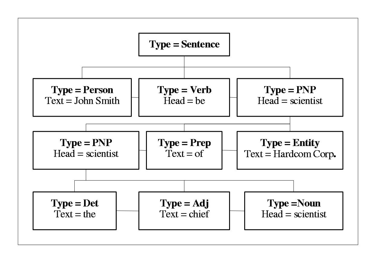
Let us consider the sentence, "John Smith is the chief scientist of the Hardcom Corporation". The shallow parsing system produces the representation of the sentence shown in Figure 1. The sentence is represented a shallow parse tree. In contrast to common parse trees, the type of a parent node does not determine the structure of its children nodes. Instead of providing the full interpretation of the sentence, shallow parsing only identifies its key elements. Therefore, shallow parsing is fairly robust, and is able to generate structured representations even for ungrammatical sentences.

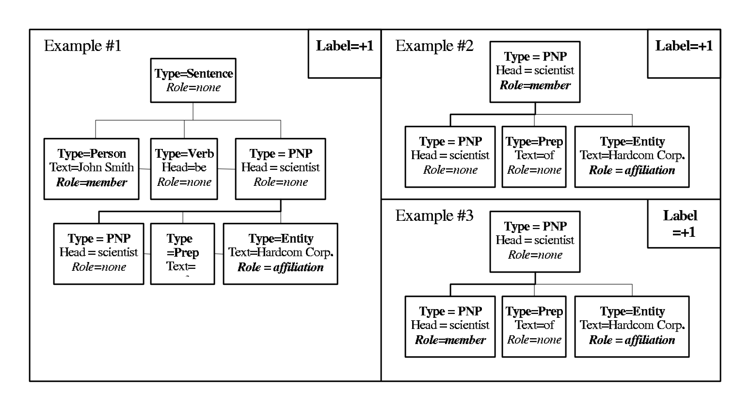
We next convert the shallow parse tree into examples for the person-affiliation relation. This type of relation holds between a person and an organization. There are three nodes in the shallow parse tree in Figure 1 referring to people, namely, the "John Smith" node with the type "Person", and the "PNP" nodes.[^5] There is one "Organization" node in the tree that refers to an organization. We create an example for the person-affiliation relation by taking a person node and an organization node in the shallow parse tree and assigning attributes to the nodes specifying the role that a node plays in the person-affiliation relation. The person and organization under consideration will receive the member and affiliation roles, respectively. The rest of the nodes will receive none roles reflecting that they do not participate in the relation. We then attach a label to the example by asking the question whether the node with the role of member and the node with the role of affiliation are indeed (semantically) affiliated, according to the sentence. For the above sentence, we will then generate three positive examples, shown in Figure 2.

[^5]: Note that after the tree is produced, we do not know if the "Person" and the "PNP" nodes refer to the same person.

Note that in generating the examples between the "PNP" and the "Organization" we eliminated the nodes that did not belong to the least common subtree of "Organization" and "PNP", thereby removing irrelevant subtrees. To summarize, a relation example is shallow parse, in which nodes are augmented with the role attribute, and each node of the shallow parse belongs to the least common subtree comprising the relation entities under consideration. We now formalize the notion of relation example. We first define the notion of the example node.

Definition 1 A node $p$ is a set of attributes ${a_1, a_2, \dots}$. Each node may have a different number of attributes. The attributes are named, and each node necessarily has attributes with names "Type" and "Role".

We use $p.a$ to denote the value of attribute with the name $a$ in the node $p$, e.g., $p.Type = Person$ and $p.Role = member$.

Definition 2 An (unlabeled) relation example is defined inductively as follows:

• Let $p$ be a node, then the pair $P = (p, [])$ is a relation example, where by $[]$ we denote an empty sequence.
• Let $p$ be a node, and $[P_1, P_2, \dots, P_l]$ be a sequence of relation examples. Then, the pair $P = (p, [P_1, P_2, \dots, P_l])$ is a relation example.

We say that $p$ is the parent of $P_1, P_2, \dots, P_l$, and $P_i

5. Kernels for Relation Extraction

Section Summary: The section introduces specialized kernels for relation extraction that operate on shallow parse trees rather than full syntactic parses. It defines a recursive similarity measure between two relation examples by first checking whether their root nodes match in type and role, then adding a node-level similarity score and a weighted sum over matching subsequences of their children; a decay factor penalizes longer or more spread-out subsequences. The authors prove that the resulting function is a valid kernel and present an efficient special case restricted to contiguous children subsequences, which they illustrate with a concrete sentence example.

Kernels on parse trees were previously defined by Collins and Duffy (2001). The kernels enumerated (implicitly) all subtrees of two parse trees, and used the number of common subtrees, weighted appropriately, as the measure of similarity between two parse trees. Since we are operating with shallow parse trees, and the focus of our problem is relation extraction rather than parsing, we use a different definition of kernels.

The nodes of the shallow parse trees have attributes, and we need to use the attributes in the kernel definition. We define a primitive kernel function on the nodes in terms of nodes' attributes, and then extend it on relation examples.

We first define a matching function $t(\cdot, \cdot) \in {0, 1}$ and a similarity function $k(\cdot, \cdot)$ on nodes. The matching function defined on nodes determines whether the nodes are matchable or not. In the case of relation extraction, the nodes are matchable only if their types and roles match. Thus, if two nodes have different roles, and non-compatible types,[^6] then their node matching function is equal to zero; otherwise, it is equal to 1. The similarity function on nodes is computed in terms of the nodes' attributes.

[^6]: Some distinct types are compatible, for example, "PNP" is compatible with "Person".

For example,

$ t(P_1.p, P_2.p) = \begin{cases} 1, & \text{if } P_1.Type = P_2.Type \text{ and } P_1.Role = P_2.Role \ 0, & \text{otherwise} \end{cases} $

and

$ k(P_1.p, P_2.p) = \begin{cases} 1, & \text{if } P_1.text = P_2.Text \ 0, & \text{otherwise} \end{cases} $

Then, for two relation examples $P_1, P_2$, we define the similarity function $K(P_1, P_2)$ in terms of similarity function of the parent nodes and the similarity function $K_c$ of the children. Formally,

$ K(P_1, P_2) = \begin{cases} 0, \text{if } t(P_1.p, P_2.p) = 0 \ k(P_1.p, P_2.p) + K_c(P_1.c, P_2.c), \text{ otherwise} \end{cases}\tag{1} $

Different definitions of the similarity function $K_c$ on children give rise to different $K

We denote by $\mathbf{i}$ a sequence $i_1 \le i_2 \le \dots \le i_n$ of indices, and we say that $i \in \mathbf{i}$, if $i$ is one of the sequence indices. We also use $d(\mathbf{i})$ for $i_n - i_1 + 1$, and $l(\mathbf{i})$ for length of the sequence $\mathbf{i}$. For a relation example $P$, we denote by $P[\mathbf{i}]$ the sequence of children $[P[i_1], \dots, P[i_n]]$.

For a similarity function $K$, we use $K(P_1[\mathbf{i}], P_2[\mathbf{j}])$ to denote $\sum_{s=1, \dots, l(\mathbf{i})} K(P_1[i_s], P_2[j_s])$. Then, we define the similarity function $K_c$ as follows

$ K_c(P_1.c, P_2.c) = \sum_{\mathbf{i}, \mathbf{j}, l(\mathbf{i})=l(\mathbf{j})} \lambda^{d(\mathbf{i})} \lambda^{d(\mathbf{j})} K(P_1[\mathbf{i}], P_2[\mathbf{j}]) \prod_{s=1, \dots, l(\mathbf{i})} t(P_1[i_s].p, P_2[j_s].p)\tag{2} $

The formula (2) enumerates all subsequences of relation example children with matching parents, accumulates the similarity for each subsequence by adding the corresponding child examples' similarities, and decreases the similarity by the factor of $\lambda^{d(\mathbf{i})} \lambda^{d(\mathbf{j})}$, $0 < \lambda < 1$, reflecting how spread out the subsequences within children sequences. Finally, the similarity of two children sequences is the sum all matching subsequences similarities.

The following theorem states that the formulas (1) and (2) define a kernel, under mild assumptions.

Theorem 3 Let $k(\cdot, \cdot)$ and $t(\cdot, \cdot)$ be kernels over nodes. Then, $K$ as defined by (1) and (2) is a kernel over relation examples.

The proof of Theorem 3 is in Appendix A.

We first consider a special case of $K_c$, where the subsequences $\mathbf{i}$ and $\mathbf{j}$ are assumed to be contiguous and give a very efficient algorithm for computing $K_c$. In Section 5.2, we address a more general case, when the subsequences are allowed to be sparse (non-contiguous).

5.1 Contiguous Subtree Kernels

For contiguous subtree kernels, the similarity function $K_c$ enumerates only children contiguous subsequences, that is, for a subsequence $\mathbf{i}$ in (2), $i_{s+1} = i_s + 1$ and $d(\mathbf{i}) = l(\mathbf{i})$. Since then $d(\mathbf{i}) = d(\mathbf{j})$ as well, we slightly abuse notation in this section by making $\lambda$ stand for $\lambda^2$ in formula (2). Hence, (2) becomes

$ K_c(P_1.c, P_2.c) = \sum_{\mathbf{i}, \mathbf{j}, l(\mathbf{i})=l(\mathbf{j})} \lambda^{l(\mathbf{i})} K(P_1[\mathbf{i}], P_2[\mathbf{j}]) \prod_{s=1, \dots, l(\mathbf{i})} t(P_1[i_s].p, P_2[j_s].p)\tag{3} $

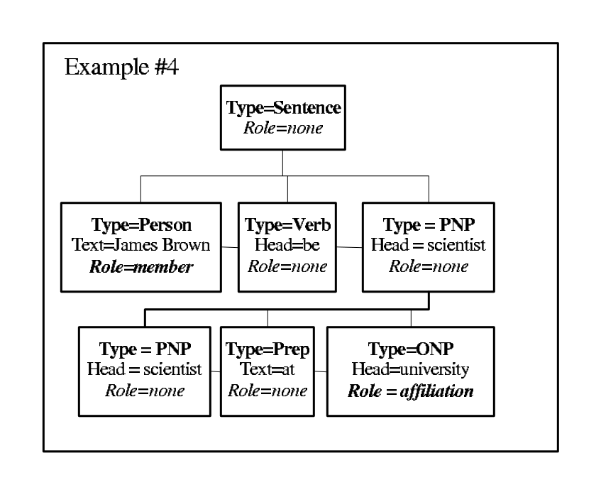
Let us consider a relation example corresponding to the sentence "James Brown was a scientist at the University of Illinois". The example is shown in Figure 3. We compare the example with the relation example #1 in Figure 2.

According to the definitions (1) and (3), for the examples $P_1$ (relation example #1) and $P_2$ (relation example #4), the kernel function is computed as follows (Assume that for all matching nodes, the similarity is 1 if their text(head) attributes match and 0, otherwise. Also assume that $\lambda = 0.5$).

$ \begin{aligned} K(P_1, P_2) &= k(P_1.Sentence.p, P_2.Sentence.p) \ &\quad + K_c([P_1.Person, P_1.Verb, P_1.PNP], [P_2.Person, P_2.Verb, P_2.PNP]) \ &= 0.5(k(P_1.Person, P_2.Person) + k(P_1.Verb, P_2.Verb) + K(P_1.PNP, P_2.PNP)) \ &\quad + 0.5^2(k(P_1.Person, P_2.Person) + 2k(P_1.Verb, P_2.Verb) + K(P_1.PNP, P_2.PNP)) \ &\quad + 0.5^3(k(P_1.Person, P_2.Person) + k(P_1.Verb, P_2.Verb) + K(P_1.PNP, P_2.PNP)) \ &= 1.125 + 0.875K(P_1.PNP, P_2.PNP) \ &= 1.125 + 0.875(k(P_1.PNP.p, P_2.PNP.p) + 0.5(k(P_1.PNP.PNP, P_2.PNP.PNP) \ &\quad + k(P_1.PNP.Prep, P_2.PNP.Prep) + k(P_1.PNP.Organization, P_2.PNP.ONP)) \ &\quad + 0.5^2(k(P_1.PNP.PNP, P_2.PNP.PNP) + 2k(P_1.PNP.Prep, P_2.PNP.Prep) \ &\quad + k(P_1.PNP.Organization, P_2.PNP.ONP)) \ &\quad + 0.5^3(k(P_1.PNP.PNP, P_2.PNP.PNP) + k(P_1.PNP.Prep, P_2.PNP.Prep) \ &\quad + k(P_1.PNP.Organization, P_2.PNP.ONP))) \ &= 1.125 + 0.875(1 + 0.5 + 0.25 + 0.125) \ &= 1.125 + 0.875 \cdot 1.875 \ &= 2.765625 \end{aligned} $

The core of the kernel computation resides in the formula (3). The formula enumerates all contiguous subsequences of two children sequences. We now give a fast algorithm for computing $K_c$ between $P_1$ and $P_2$, which, given kernel values for children, runs in time $O(mn)$, where $m$ and $n$ is the number of children of $P_1$ and $P_2$, respectively.

Let $C(i, j)$ be the $K_c$ computed for suffixes of children sequences of $P_1$ and $P_2$, where every subsequence starts with indices $i$ and $j$, respectively. That is,

$ C(i, j) = \sum_{\mathbf{i}, \mathbf{j}, i_1=i, j_1=j, l(\mathbf{i})=l(\mathbf{j})} \lambda^{l(\mathbf{i})} K(P_1[\mathbf{i}], P_2[\mathbf{j}]) \prod_{s=1, \dots, l(\mathbf{i})} t(P_1[i_s].p, P_2[j_s].p) $

Let $L(i, j)$ be the length of the longest sequence matching states in the children of $P_1$ and $P_2$ starting with indices $i$ and $j$, respectively. Formally,

$ L(i, j) = \max{l : \prod_{s=0, \dots, l} t(P_1[i+s].p, P_2[j+s].p) = 1} $

Then, the following recurrences hold:

$ L(i, j) = \begin{cases} 0, \text{ if } t(P_1[i].p, P_2[j].p) = 0 \ L(i+1, j+1) + 1, \text{ otherwise} \end{cases}\tag{4} $

$ C(i, j) = \begin{cases} 0, \text{if } t(P_1[i].p, P_2[j].p) = 0 \ \frac{\lambda(1-\lambda^{L(i, j)})}{1-\lambda} K(P_1[i], P_2[j]) + \lambda C(i+1, j+1), \text{ otherwise} \end{cases}\tag{5} $

The boundary conditions are:

$ L(m+1, n+1) = 0 $

$ C(m+1, n+1) = 0 $

The recurrence (5) follows from the observation that, if $P_1[i]$ and $P_2[j]$ match, then every matching pair $(c_1, c_2)$ of sequences that participated in computation of $C(i+1, j+1)$ will be extended to the matching pair $([P_1[i], c_1], [P_2[j], c_2])$, and

$ \begin{aligned} C(i, j) &= \lambda K(P_1[i], P_2[j]) + \sum_{(c_1, c_2)} \lambda^{l(c_1)+1}(K(P_1[i], P_2[j]) + K(c_1, c_2)) \ &= \sum_{s=1, \dots, L(i, j)} \lambda^s K(P_1[i], P_2[j]) + \lambda \sum_{(c_1, c_2)} \lambda^{l(c_1)} K(c_1, c_2) \ &= \frac{\lambda(1-\lambda^{L(i, j)})}{1-\lambda} K(P_1[i], P_2[j]) + \lambda C(i+1, j+1) \end{aligned} $

Now we can easily compute $K_c(P_1.c, P_2.c)$ from $C(i, j)$.

$ K_c(P_1.c, P_2.c) = \sum_{i, j} C(i, j)\tag{6} $

The time and space complexity of $K_c$ computation is $O(mn)$, given kernel values for children. Hence, for two relation examples the complexity of computing $K(P_1, P_2)$ is the sum of computing $K_c$ for the matching internal nodes (assuming that complexity of $t(\cdot, \cdot)$ and $k(\cdot, \cdot)$ is constant).

5.2 Sparse Subtree Kernels

For sparse subtree kernels, we use the general definition of similarity between children sequences as expressed by (2).

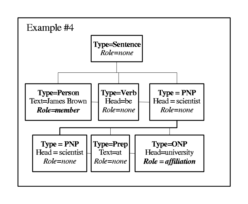
Let us consider a example corresponding to the sentence "John White, a well-known scientist at the University of Illinois, led the discussion." The example is shown in Figure 4. We compare the example with the relation example #1 in Figure 2.

According to the definitions (1) and (3), for the examples $P_1$ (relation example #1) and $P_2$ (relation example #5), the kernel function is computed as follows (Assume that for all matching nodes, the similarity is 1 if their text(head) attributes match and 0, otherwise. Also assume that $\lambda = 0.5$).

$ \begin{aligned} K(P_1, P_2) &= k(P_1.Sentence.p, P_2.Sentence.p) + \ &\quad + K_c([P_1.Person, P_1.Verb, P_1.PNP], [P_2.Person, P_2.Punc, P_2.PNP, P_2.Verb, P_2.BNP]) \ &= 0.5^2(k(P_1.Person, P_2.Person) + k(P_1.Verb, P_2.Verb) + K(P_1.PNP, P_2.PNP)) \ &\quad + 0.5^2 0.5^4 k([P_1.Person, P_1.Verb], [P_2.Person, P_2.Verb]) + \ &\quad + 0.5^3 0.5^3([P_1.Person, P_1.PNP], [P_2.Person, P_2.PNP]) + \ &\quad + (0.5^2 + 0.5^6) K(P_1.PNP, P_2.PNP) \ &= 0.265625(k(P_1.PNP.p, P_2.PNP.p) + 0.5^2(k(P_1.PNP.PNP, P_2.PNP.PNP) \ &\quad + k(P_1.PNP.Prep, P_2.PNP.Prep) + k(P_1.PNP.ONP, P_2.PNP.ONP)) \ &\quad + 0.5^4(k(P_1.PNP.PNP, P_2.PNP.PNP) + 2k(P_1.PNP.Prep, P_2.PNP.Prep) \ &\quad + k(P_1.PNP.ONP, P_2.PNP.ONP)) + 0.5^6(k(P_1.PNP.PNP, P_2.PNP.PNP) + \ &\quad + k(P_1.PNP.ONP, P_2.PNP.ONP)) + \ &\quad + 0.5^6(k(P_1.PNP.PNP, P_2.PNP.PNP) + k(P_1.PNP.Prep, P_2.PNP.Prep) \ &\quad + k(P_1.PNP.ONP, P_2.PNP.ONP)) \ &= 0.265625(1 + 0.5^2 \cdot 3 + 0.5^4 \cdot 4 + 0.5^6 \cdot (2 + 3)) \ &= 0.265625 \cdot 2.078125 \ &= 0.552 \end{aligned} $

As in the previous section, we give an efficient algorithm for computing $K_c$ between $P_1$ and $P_2$. The algorithm runs in time $O(mn^3)$, given kernel values for children, where $m$ and $n$ ($m \ge n$) is the number of children of $P_1$ and $P_2$, respectively. We will use a construction of Lodhi et al. (2002) in the algorithm design.

Derivation of an efficient programming algorithm for sparse subtree computation is somewhat involved and presented in Appendix B. Below we list the recurrences for computing $K_c$.

$ K_c = \sum_{q=1, \dots, \min(m, n)} K_{c, q}(m, n) $

$ K_{c, q}(i, j) = \lambda K_{c, q}(i, j - 1) + \sum_{s=1, \dots, i} t(P_1[s].p, P_2[j].p) \lambda^2 C_{q-1}(s - 1, j - 1, K(P_1[s], P_2[j])) $

$ C_q(i, j, a) = a C_q(i, j) + \sum_{r=1, \dots, q} C_{q, r}(i, j) $

$ C_q(i, j) = \lambda C_q(i, j - 1) + C_q'(i, j) $

$ C_q'(i, j) = t(P_1[i], P_2[j]) \lambda^2 C_{q-1}(i - 1, j - 1) + \lambda C_q'(i, j - 1) $

$ C_{q, r}(i, j) = \lambda C_{q, r}(i, j - 1) + C_{q, r}'(i, j) $

$ C_{q, r}'(i, j) = \begin{cases} t(P_1[i], P_2[j]) \lambda^2 C_{q-1, r}(i - 1, j - 1) + \lambda C_{q, r}'(i, j - 1), & \text{if } q \ne r \ t(P_1[i], P_2[j]) \lambda^2 K(P_1[i], P_2[j]) C_{q-1}(i - 1, j - 1) + \lambda C_{q, r}'(i, j - 1), & \text{if } q = r \end{cases} $

The boundary conditions are

$ K_{c, q}(i, j) = 0, \text{ if } q > \min(i, j) $

$ C_q(i, j) = 0, \text{ if } q > \min(i, j) $

$ C_0(i, j) = 1, $

$ C_q'(i, j) = 0, \text{ if } q > \min(i, j) $

$ C_{q, r}(i, j) = 0, \text{ if } q > \min(i, j) \text{ or } q < r $

$ C_{q, r}'(i, j) = 0, \text{ if } q > \min(i, j) \text{ or } q < r $

As can be seen from the recurrences, the time complexity of the algorithm is $O(mn^3)$ (assuming $m \ge n$). The space complexity is $O(mn^2)$.

6. Experiments

Section Summary: The experiments test kernel-based learning methods on the task of extracting two nuanced relations—person-affiliation and organization-location—from a collection of 200 news articles that were shallow-parsed and manually labeled. Examples were randomly divided into training and test sets, and performance was measured with precision, recall, and F-measure across multiple splits while also tracking how results improved with more training data. Two kernel algorithms, support vector machines and voted perceptrons using contiguous and sparse subtree kernels, were compared against conventional feature-based approaches to assess whether the kernels’ ability to consider larger substructures yields better extraction accuracy.

In this section, we apply kernel methods to extracting two types of relations from text: person-affiliation and organization-location.

A person and an organization are part of the person-affiliation relation, if the person is a member of or employed by organization. A company founder, for example, is defined not to be affiliated with the company (unless, it is stated that (s)he also happens to be a company employee).

A organization and a location are components of the organization-location relation, if the organization's headquarters is at the location. Hence, if a single division of a company is located in a particular city, the company is not necessarily located in the city.

The nuances in the above relation definitions make the extraction problem more difficult, but they also allow to make fine-grained distinctions between relationships that connect entities in text.

6.1 Experimental Methodology

The (text) corpus for our experiments comprises 200 news articles from different news agencies and publications (Associated Press, Wall Street Journal, Washington Post, Los Angeles Times, Philadelphia Inquirer).

We used the existing shallow parsing system to generate the shallow parses for the news articles. We generated relation examples from the shallow parses for both relations, as described in Section 4. We retained only the examples, for which the shallow parsing system did not make major mistakes (90% of the generated examples). We then labeled the retained examples whether they expressed the relation of interest. The resulting examples' statistics are shown in Table 6.1.

: Table 1: Number of examples for relations.

\begin{tabular}{|l|c|c|}
\hline
 & person-affiliation & org-location \\
\hline
\#positive & 1262 & 506 \\
\#negative & 2262 & 1409 \\
\hline
\#total & 3524 & 1915 \\
\hline
\end{tabular}

For each relation, we randomly split the set of examples into a training set (60% of the examples) and a testing set (40% of the examples). We obtained the models by running learning algorithms (with kernels, where appropriate) on the training set, testing the models on the test set, and computing performance measures. In order to get stable performance estimates, we averaged performance results over 10 random train/test splits. For each of the algorithms, we also computed the learning curves by gradually increasing the number of examples in the training set and observing performance change on the test set. The learning curves were also averaged over 10 random train/test splits.

For extraction problems, the system performance is usually reflected using the performance measures of information retrieval: precision, recall, and F-measure (van Rijsbergen, 1979). Precision is the ratio of the number of correctly predicted positive examples to the number predicted positive examples. Recall is the ratio of the number of correctly predicted positive examples to the number of true positive examples. F-measure (Fm) combines precision and recall as follows:

$ Fm = \frac{2 * precision * recall}{(precision + recall)} $

We report precision, recall, and F-measure for each experiment. We also present F-measure learning curves for each learning curve experiment.

In the experiments below, we present the performance of kernel-based algorithms for relation extraction in conjunction with that of feature-based algorithms. Note that the set of features used by the feature-based learning algorithms (presented in Appendix C) is not the same as the set of implicit features employed by kernel-based learning algorithms. The features used correspond to small subtrees of the shallow parse representations of relation examples, while the kernel formulation can take advantage of subtrees of any size. Therefore, in comparing the performance of kernel-based and feature-based methods, we seek to evaluate how much advantage a kernel formulation can give us with respect to a comparable yet less expressive feature formulation.

We now describe the experimental setup of the algorithms used in evaluation.

6.2 Kernel Methods Configuration

We evaluated two kernel learning algorithms: Support Vector Machine (SVM) (Cortes and Vapnik, 1995) and Voted Perceptron (Freund and Schapire, 1999). For SVM, we used the $SVM^{Light}$ (Joachims, 1998) implementation of the algorithm, with custom kernels incorporated therein. We implemented the Voted Perceptron algorithm as described in (Freund and Schapire, 1999).

We implemented both contiguous and sparse subtree kernels and incorporated them in the kernel learning algorithms. For both kernels, $\lambda$ was set to 0.5. The only domain specific information in the two kernels was encapsulated by the matching $t(\cdot, \cdot)$ and similarity $k(\cdot, \cdot)$ functions on nodes. Both functions are extremely simple, their definitions are shown below.

$ t(P_1.p, P_2.p) = \begin{cases} 1, & \text{if } Class(P_1.Type) = Class(P_2.Type) \text{ and } P_1.Role = P_2.Role \ 0, & \text{otherwise} \end{cases} $

where the function $Class$ combines some types into a single equivalence class: $Class(\text{PNP}) = \text{Person}$, $Class(\text{ONP}) = \text{Organization}$, $Class(\text{LNP}) = \text{Location}$, and $Class(\text{Type}) = \text{Type}$ for other types.

$ k(P_1.p, P_2.p) = \begin{cases} 1, & \text{if } P_1.text = P_2.Text \ 0, & \text{otherwise} \end{cases} $

We should emphasize that the above definitions of $t$ and $k$ are the only domain-specific information that the kernel methods use. Certainly, the kernel design is somewhat influenced by the problem of relation extraction, but the kernels can be used for other (not necessarily text-related) problems as well, if the functions $t$ and $k$ are defined differently.

We also normalized the computed kernels before their use within the algorithms. The normalization corresponds to the standard unit norm normalization of examples in the feature space corresponding to the kernel space (Cristianini and Shawe-Taylor, 2000):

$ K(P_1, P_2) = \frac{K(P_1, P_2)}{\sqrt{K(P_1, P_1) K(P_2, P_2)}} $

For both $SVM^{Light}$ and Voted Perceptron, we used their standard configurations (e.g., we did not optimize the value of $C$ that interpolates the training error and regularization cost for SVM, via cross-validation). For Voted Perceptron, we performed two passes over the training set.

6.3 Linear Methods Configuration

We evaluated three feature-based algorithms for learning linear discriminant functions: Naive-Bayes (Duda and Hart, 1973), Winnow (Littlestone, 1987), and SVM. We designed features for the relation extraction problem. The features are conjunctions of conditions defined over relation example nodes. The features are listed in appendix C. Again, we use the standard configuration for both algorithms: for Naive Bayes we employed add-one smoothing (Jelinek, 1997); for Winnow, learning rate (promotion parameter) was set to 1.1 and the number of training set passes to 2. For SVM, we used the linear kernel and set the regularization parameter ($C$) to 1.

6.4 Experimental Results

The performance results for person-affiliation and organization-location are shown in Table 2 and Table 3, respectively. The results indicate that kernel methods do exhibit good performance and, in most cases, fare better than feature-based algorithms in relation extraction. The results also highlights importance of kernels: algorithms with the sparse subtree kernels are always significantly better than their contiguous counterparts. The SVM results also pinpoint that kernels and not regularization are crucial for performance improvement.

: Table 2: Person-affiliation performance (in percentage points)

\begin{tabular}{|l|c|c|c|}
\hline
 & Recall & Precision & F-measure \\
\hline
Naive Bayes & 75.59 & 91.88 & 82.93 \\
Winnow & 80.87 & 88.42 & 84.46 \\
SVM (feature-based) & 76.21 & 91.67 & 83.22 \\
Voted Perceptron (contiguous) & 79.58 & 89.74 & 84.34 \\
SVM (contiguous) & 79.78 & 89.9 & 84.52 \\
Voted Perceptron (sparse) & 81.62 & 90.05 & 85.61 \\
SVM (sparse) & 82.73 & 91.32 & \textbf{86.8} \\
\hline
\end{tabular}

: Table 3: Organization-location performance (in percentage points)

\begin{tabular}{|l|c|c|c|}
\hline
 & Recall & Precision & F-measure \\
\hline
Naive Bayes & 71.94 & 90.40 & 80.04 \\
Winnow & 75.14 & 85.02 & 79.71 \\
SVM (feature-based) & 70.32 & 88.18 & 78.17 \\
Voted Perceptron (contiguous) & 64.43 & 92.85 & 76.02 \\
SVM (contiguous) & 71.43 & 92.03 & 80.39 \\
Voted Perceptron (sparse) & 71 & 91.9 & 80.05 \\
SVM (sparse) & 76.33 & 91.78 & \textbf{83.3} \\
\hline
\end{tabular}

6.4.1 Feature-Based vs. Kernel-Based: Learning Curves

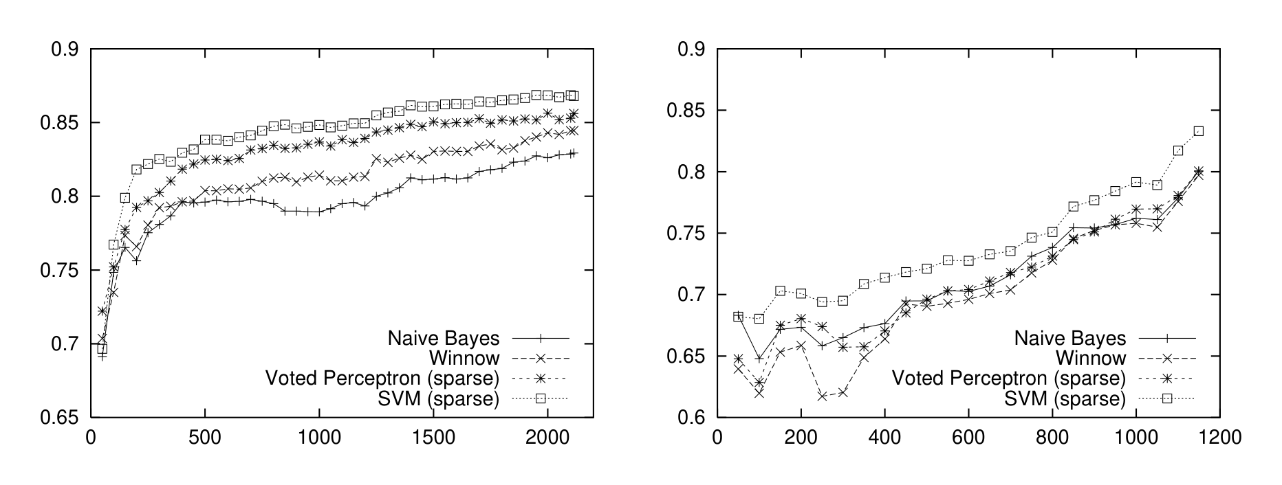
The Figure 5 depicts F-measure learning curves for for feature-based and kernel-based algorithms with the sparse subtree kernel.

For the person-affiliation relation, kernel-based algorithms clearly outperform feature-based algorithms starting just from just a hundred examples. The kernel-based algorithms converge faster, and they are more stable, if trained on few examples. For the organization-location relation, the trend is less clear for the Voted Perceptron, whose performance, with the sparse subtree kernel, is just comparable to that of feature-based algorithms. SVM, with the sparse subtree kernel, performs far better than any of the competitors for the organization-location relation.

6.4.2 Sparse vs. Contiguous: Learning Curves

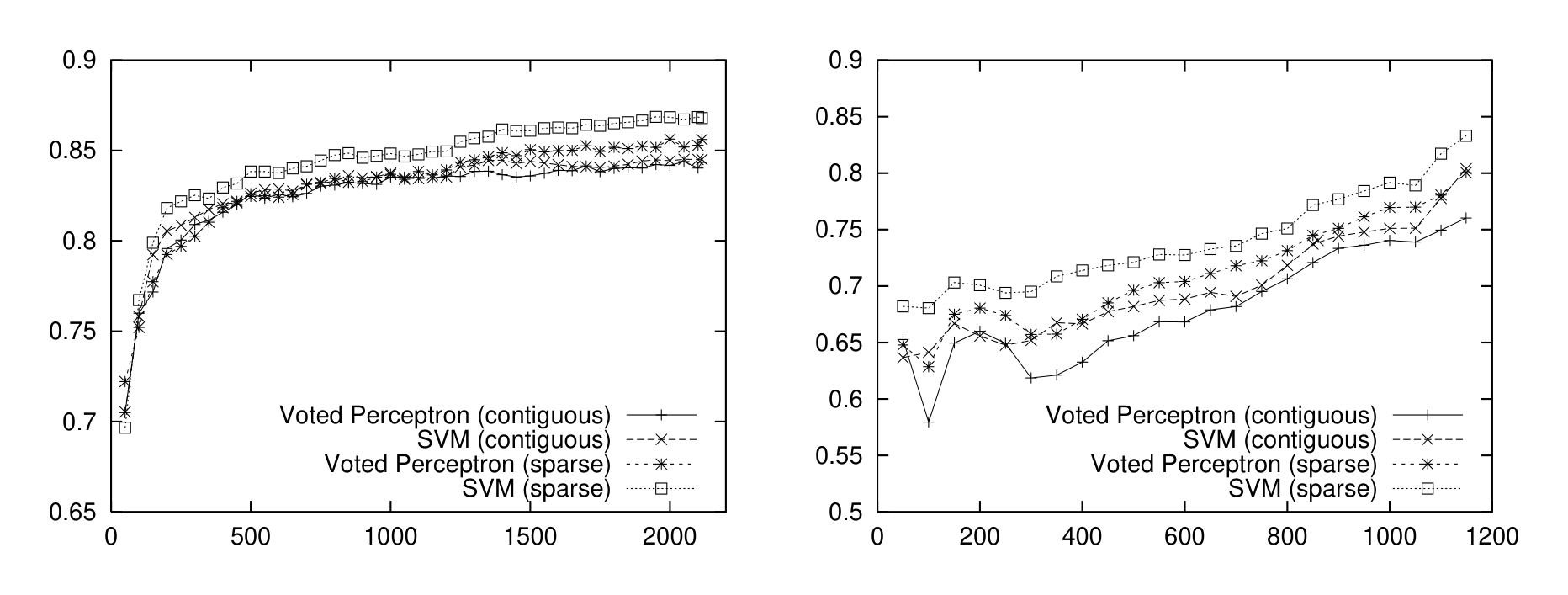
The Figure 6 depicts F-measure learning curves for for kernel-based algorithms algorithms with different kernels.

The learning curves indicate that the sparse subtree kernel is far superior to the contiguous subtree kernel. From the enumeration standpoint, the subtree kernels implicitly enumerate the exponential number of children subsequences of a given parent, while the contiguous kernels essentially operate with $n$-grams, whose number is just quadratic in a children sequence length. This exponential gap between the sparse and contiguous kernels leads to a significant performance improvement. The result is extremely promising, for it showcases that it is possible to (implicitly) consider an exponential number of features while paying just a low polynomial price, with a significant performance boost.

7. Discussion

Section Summary: Kernel methods provide an effective way to learn from the inherent structure of language in tasks like relation extraction, without relying on heavy feature engineering or simplified representations. They can achieve strong results with fewer examples than some traditional approaches, though their practical use is hindered by slower speeds when applied to very large datasets. Future work could adapt distance measures from other fields, such as bioinformatics, to design more efficient kernels suited to natural language processing.

Kernel-based methods are an elegant approach for learning in rich structural domains. Our results show that, for relation extraction, the methods perform very well, while allowing for minimal ingestion of problem knowledge and avoidance of extensive feature engineering and selection process. Our work follows recent applications of kernel methods to natural language parsing (Collins and Duffy, 2001) and text categorization (Lodhi et al., 2002). The common theme in all the papers is that objects' structure need not be sacrificed for simpler explicit feature-based representation. Indeed, the structure can be leveraged in a computationally efficient and statistically sound way.

The NLP domain is precisely the domain where the structural descriptions of objects (words, phrases, sentences) can be exploited. While the prevalent $n$-grams approach to language modeling imposes statistical and computational constraints, kernel-based language modeling may help eschew the constraints. We have shown that, for relation extraction, the kernel algorithms exhibit faster convergence than such attribute-efficient[^7] algorithms as Winnow. We hypothesize that the methods will require much fewer examples in achieving the state of the art performance for a range of NLP problems than approaches based on probabilistic modeling.

[^7]: A learning algorithm is attribute-efficient, if its learning rate depends on the number of relevant features, rather than on the total number of features.

One practical problem in applying kernel methods to NLP is their speed. Kernel classifiers are relatively slow compared to feature classifiers. Indeed, an application of a kernel classifier requires evaluation of numerous kernels whose computational complexity may be too high for practical purposes. Many low level problems in natural language processing involve very large corpora with tens and hundreds of thousands of examples. Even if kernel classifiers only depend on a small subset of the examples (for instance, support vectors of SVM), the need to evaluate thousands of complex kernels during the classifier application may render kernel methods inappropriate for various practical settings. Therefore, there is a pressing need to develop algorithms that combine the advantages of kernel methods with practical constraints that require efficient application of the classifiers learned.

Design of kernels for structural domains is a very rich research area. An interesting direction to pursue would be to use extensive work on distances defined on structural objects (Sankoff and Kruskal, 1999) in kernel design. The distance-based methods have already found widespread application in bioinformatics (Durbin et al., 1998), and can be fruitfully extended to work in the NLP domain as well. Watkins (1999) presents sufficient conditions for a Pair Hidden Markov Model (which is a probabilistic version of edit distance) to constitute a kernel. More generally, the work of Goldfarb (1985) makes it possible to use any distance measure to embed objects (and define a dot product) in a pseudo-euclidean space. Incidentally, SVM can be adapted for the pseudo-euclidean representations (Graepel et al., 1999, Pekalska et al., 2001), hence, lending the power of regularization to learning in structural domains, where natural distance functions exist.

8. Conclusions and Further Work

Section Summary: The authors described a new kernel-based machine learning method for pulling out relations from text by operating on shallow parse structures, with efficient algorithms to compute the kernels and strong results when paired with SVM and voted perceptron classifiers. They showed that this approach outperformed traditional feature-based methods on relation extraction tasks. Looking ahead, they plan to extend the same kernel techniques to related problems such as learning shallow parsing and entity detection jointly and handling discourse-level tasks like resolving entities, noun phrases, and pronouns.

We presented an approach for using kernel-based machine learning methods for extracting relations from natural language sources. We defined kernels over shallow parse representations of text and designed efficient dynamic programming algorithms for computing the kernels. We applied SVM and Voted Perceptron learning algorithms with the kernels incorporated therein to the tasks of relation extraction. We also compared performance of the kernel-based methods with that of the feature methods, and concluded that kernels lead to superior performance.

Aside from a number of interesting research directions mentioned in Section 7, we intend to apply the kernel methodology to other sub-problems of information extraction. For example, the shallow parsing and entity extraction mechanism may also be learned, and, perhaps, combined in a seamless fashion with the relation extraction formalism presented herein. Furthermore, the real-world use of extraction results requires discourse resolution that collapses entities, noun phrases, and pronouns into a set of equivalence classes. We plan to apply kernel methods for discourse processing as well.

9. Acknowledgments

This work was supported through the DARPA Evidence Extraction and Link Discovery program under the contract 2001-H697000-000.

Appendix A. Proof of Theorem 3

Section Summary: The proof shows that the function K qualifies as a valid kernel on relation examples by building directly on standard closure properties of kernels under sums, products, direct sums, and tensor products. In the base case where at least one example has no children, K reduces to a simple product of two existing kernels and is therefore itself a kernel. For examples with children, the children component is rewritten as a sum over padded subsequences; each term is shown to be a kernel via the cited lemmas and corollaries, the sum itself is a kernel by an additional lemma on kernels over sets, and the full expression for K is again closed under the same operations.

To prove the theorem, we need the following lemmas.

Lemma 4 (Haussler (1999)) Let $K$ be a kernel on a set $U \times U$ and for all finite non-empty $A, B \subseteq U$ define $\bar{K}(A, B) = \sum_{x \in A, y \in B} K(x, y)$. Then $\bar{K}$ is the kernel on the product of the set of all finite, nonempty subsets of $U$ with itself.

Lemma 5 (Cristianini and Shawe-Taylor (2000)) If $K_1$ is a kernel over a set $X$, and $K_2$ is a kernel over a set $Y$, then $K_1 \oplus K_2((x, x'), (y, y')) = K(x, x') + K(y, y')$ is a kernel over a set $X \times Y$. The kernel $K_1 \oplus K_2$ is called the direct sum of kernels $K_1$ and $K_2$.

Corollary 6 If $K_1, \dots, K_n$ are kernels over the corresponding sets $X_1, \dots, X_n$, and then the direct sum $K_1 \oplus \dots \oplus K_n((x_1, x_1'), \dots, (x_n, x_n')) = \sum_{i=1, \dots, n} K(x_i, x_i')$ is a kernel over the set $X_1 \times \dots \times X_n$.

Lemma 7 (Cristianini and Shawe-Taylor (2000)) If $K_1$ is a kernel over a set $X$, and $K_2$ is a kernel over a set $Y$, then $K_1 \otimes K_2((x, x'), (y, y')) = K(x, x') K(y, y')$ is a kernel over a set $X \times Y$. The kernel $K_1 \otimes K_2$ is called the tensor product of kernels $K_1$ and $K_2$.

Corollary 8 If $K_1, \dots, K_n$ are kernels over the corresponding sets $X_1, \dots, X_n$, and then the tensor product $K_1 \otimes \dots \otimes K_n((x_1, x_1'), \dots, (x_n, x_n')) = \prod_{i=1, \dots, n} K(x_i, x_i')$ is a kernel over the set $X_1 \times \dots \times X_n$.

Proof [Proof of Theorem 3] For two relation examples $P_1$ and $P_2$, of which at least one has no children, $K(P_1, P_2) = k(P_1.p, P_2.p)t(P_1.p, P_2.p)$. Therefore, $K$ is a kernel as a product of two kernels(Cristianini and Shawe-Taylor, 2000).

For two relation examples $P_1$ and $P_2$ with non-empty children lists, we first extend each children subsequence to be of length $M = \max(l(P_1.c), l(P_2.c))$ by appending to it a sequence of "empty" children, thereby embedding the space of all subsequences in the space of subsequences of length $M$. We also extend the $t(\cdot, \cdot)$ and $k(\cdot, \cdot)$ to empty nodes by making empty nodes match only with empty nodes, and putting $k(x, y) = 0$, if $x$ or $y$ is empty. We also let $d(\mathbf{i})$ denote $i_n - i_1 + 1$, where $i_n$ is the last "non-empty" index of the sequence $\mathbf{i}$.

We then observe that $K_c(P_1.c, P_2.c)$ can be written as

$ K_c(P_1.c, P_2.c) = \sum_{\mathbf{i}, \mathbf{j}} \lambda^{d(\mathbf{i})} \lambda^{d(\mathbf{j})} K(P_1[\mathbf{i}], P_2[\mathbf{j}]) \prod_{s=1, \dots, M} t(P_1[i_s].p, P_2[j_s].p) $

$K(P_1[\mathbf{i}], P_2[\mathbf{j}])$ is a direct sum of kernels defined over individual children, hence, it is a kernel over subsequences children by Corollary 6. Similarly, $\prod_{s=1, \dots, l(\mathbf{i})} t(P_1[i_s].p, P_2[j_s].p)$ is a tensor product of kernels, hence, it is a kernel over subsequences of children by Corollary 8. Since the set of kernels is closed with respect to product and scalar multiplication, $\lambda^{d(\mathbf{i})} \lambda^{d(\mathbf{j})} K(P_1[\mathbf{i}], P_2[\mathbf{j}]) \prod_{s=1, \dots, M} t(P_1[i_s].p, P_2[j_s].p)$ is a kernel over subsequences of children. Application of Lemma 4 to this kernel, where $U$ is the set of subsequences of children entails that $K_c$ is a kernel over two children sequences represented as sets of their subsequences.

Finally, since a sum and a product of kernels is also a kernel,

$ K(P_1, P_2) = t(P_1.p, P_2.p)k(P_1.p, P_2.p) + t(P_1.p, P_2.p)K_c(P_1.c, P_2.c) $

is a kernel over relation examples.

Appendix B. Sparse Subtree Kernel Computation

Section Summary: The appendix presents dynamic programming recurrences for computing the sparse subtree kernel K_c between two trees by matching ordered subsequences of their children. It begins with auxiliary quantities C_q(i,j,a) that incorporate an additive offset a inside each child-kernel evaluation, then algebraically decomposes these into separate terms C_q and C_{q,r} that remove the offset and reduce to the string subsequence kernel of Lodhi et al. together with a small number of auxiliary arrays updated in linear passes. The resulting O(qmn) procedure, together with the listed base cases, yields the final kernel value as the sum of the length-q contributions.

Let $K_{c, q}(i, j)$ be $K_c$ computed using subsequences of length $q$ in prefixes of children sequences of $P_1$ and $P_2$ ending with indices $i$ and $j$.

$ K_{c, q}(i, j) = \sum_{\mathbf{i} \subseteq {1, \dots, i}} \sum_{\substack{\mathbf{j} \subseteq {1, \dots, j} \ l(\mathbf{i})=l(\mathbf{j})=q}} \lambda^{d(\mathbf{i})} \lambda^{d(\mathbf{j})} K(P_1[\mathbf{i}], P_2[\mathbf{j}]) T(\mathbf{i}, \mathbf{j}) $

where

$ T(\mathbf{i}, \mathbf{j}) = \prod_{s=1, \dots, l(\mathbf{i})} t(P_1[i_s].p, P_2[j_s].p) $

Let $C_q(i, j, a)$ be the $K_c$ computed using subsequences of length $q$ in prefixes of children sequences of $P_1$ and $P_2$ ending with indices $i$ and $j$, respectively, with a number $a \in \mathbb{R}$ added to each result of kernel children computation, and setting a damping factor for a sequence $\mathbf{i}(\mathbf{j})$ to be $\lambda^{i-i_1+1}(\lambda^{i-i_1+1})$. Formally,

$ C_q(i, j, a) = \sum_{\mathbf{i} \subseteq {1, \dots, i}} \sum_{\substack{\mathbf{j} \subseteq {1, \dots, j} \ l(\mathbf{i})=l(\mathbf{j})=q}} [\lambda^{i-i_1+j-j_1+2}(K(P_1[\mathbf{i}], P_2[\mathbf{j}]) + a) T(\mathbf{i}, \mathbf{j})] $

Then the following recurrences hold:

$ C_0(i, j, a) = a $

$ C_q(i, j, a) = \lambda C_q(i, j - 1, a) + \sum_{s=1, \dots, i} [t(P_1[s].p, P_2[j].p) \lambda^{i-s+2} \cdot C_{q-1}(s - 1, j - 1, a + K(P_1[s], P_2[j]))] $

$ K_{c, q}(i, j) = \lambda K_{c, q}(i, j - 1) + \sum_{s=1, \dots, i} [t(P_1[s].p, P_2[j].p) \lambda^2 \cdot C_{q-1}(s - 1, j - 1, K(P_1[s], P_2[j]))] $

$ K_c = \sum_{q=1, \dots, \min(m, n)} K_{c, q}(m, n) $

The above recurrences do not allow, however, for an efficient algorithm in computing $K_c$ due to presence of real-valued parameter $a$.

In order to obtain an efficient dynamic programming algorithm, we rewrite $C_q(i, j, a)$ as follows:

$ C_q(i, j, a) = a C_q(i, j) + \sum_{r=1, \dots, q} C_{q, r}(i, j) $

where

$ C_q(i, j) = \sum_{\mathbf{i} \subseteq {1, \dots, i}} \sum_{\substack{\mathbf{j} \subseteq {1, \dots, j} \ l(\mathbf{i})=l(\mathbf{j})=q}} \lambda^{d(\mathbf{i})} \lambda^{d(\mathbf{j})} T(\mathbf{i}, \mathbf{j}) $

and

$ C_{q, r}(i, j) = \begin{cases} \sum_{\substack{i_1=1, \dots, i \ j_1=1, \dots, j}} [t(P_1[i_1].p, P_2[j_1].p) \lambda^{i-i_1+j-j_1+2} C_{q-1, r}(i_1 - 1, j_1 - 1)], & \text{if } q \ne r \ \sum_{\substack{i_1=1, \dots, i \ j_1=1, \dots, j}} [t(P_1[i_1].p, P_2[j_1].p) \lambda^{i-i_1+j-j_1+2} K(P_1[i_1], P_2[j_1]) C_{q-1}(i_1 - 1, j_1 - 1)], & \text{if } q = r \end{cases} $

Observe that $C_q(i, j)$ computes the subsequence kernel of Lodhi et al. (2002) (with matching nodes) for prefixes of $P_1$ and $P_2$. Hence, we can use the result of Lodhi et al. (2002) to give $O(qij)$ for $C_q(i, j)$ computation. Denote

$ C_q'(i, j) = \sum_{s=1, \dots, i} t(P_1[s].p, P_2[j].p) \lambda^{i-s+2} C_{q-1}(s - 1, j - 1) $

Then

$ C_q(i, j) = \lambda C_q(i, j - 1) + C_q'(i, j) $

and

$ C_q'(i, j) = t(P_1[i], P_2[j]) \lambda^2 C_{q-1}(i - 1, j - 1) + \lambda C_q'(i, j - 1) $

Using the same trick for $C_{q, r}(i, j)$, we get

$ C_{q, r}(i, j) = \lambda C_{q, r}(i, j - 1) + C_{q, r}'(i, j) $

where

$ C_{q, r}'(i, j) = \begin{cases} \lambda C_{q, r}'(i, j - 1) + t(P_1[i], P_2[j]) \lambda^2 C_{q-1, r}(i - 1, j - 1), & \text{if } q \ne r \ \lambda C_{q, r}'(i, j - 1) + t(P_1[i], P_2[j]) \lambda^2 K(P_1[i], P_2[j]) C_{q-1}(i - 1, j - 1), & \text{o.w.} \end{cases} $

That completes our list of recurrences of computing $K_q(i, j, a)$. The boundary conditions are

$ K_{c, q}(i, j) = 0, \text{ if } q > \min(i, j) $

$ C_q(i, j) = 0, \text{ if } q > \min(i, j) $

$ C_0(i, j) = 1, $

$ C_q'(i, j) = 0, \text{ if } q > \min(i, j) $

$ C_{q, r}(i, j) = 0, \text{ if } q > \min(i, j) \text{ or } q < r $

$ C_{q, r}'(i, j) = 0, \text{ if } q > \min(i, j) \text{ or } q < r $

Appendix C. Features for Relation Extraction

Section Summary: The appendix describes a set of engineered features for relation extraction that rely on the depth of each node within a tree-structured example. Individual nodes contribute features combining their depth with type, role, and text attributes, while pairs and triples of nodes add further indicators for direct parent-child links and ordered sibling sequences. Together these capture both standalone node properties and local structural patterns to help identify relations.

In the process of feature engineering, we found the concept of node depth (in a relation example) to be very useful. The depth of a node $P_1.p$ (denoted $depth(P_1.p)$) within a relation example $P$ is the depth of $P_1$ in the tree of $P$. The features are itemized below (the lowercase variables $text$, $type$, $role$, and $depth$ are instantiated with specific values for the corresponding attributes).

• For every node $P_1.p$ in a relation example, add the following features:

  • $depth(P_1.p) = depth \land Class(P_1.Type) = type \land P_1.Role = role$
  • $depth(P_1.p) = depth \land P_1.Text = text \land P_1.Role = role$

• For every pair of nodes $P_1.p$, $P_2.p$ in a relation example, such that $P_1$ is the parent of $P_2$, add the following features:

  • $depth(P_1.p) = depth \land Class(P_1.Type) = type \land P_1.Role = role \land depth(P_2.p) = depth \land Class(P_2.Type) = type \land P_2.Role = role \land parent$
  • $depth(P_1.p) = depth \land Class(P_1.Type) = type \land P_1.Role = role \land depth(P_2.p) = depth \land P_2.Text = text \land P_2.Role = role \land parent$
  • $depth(P_1.p) = depth \land P_1.Text = text \land P_1.Role = role \land depth(P_2.p) = depth \land Class(P_2.Type) = type \land P_2.Role = role \land parent$
  • $depth(P_1.p) = depth \land Class(P_1.Type) = text \land P_1.Role = role \land depth(P_2.p) = depth \land P_2.Text = text \land P_2.Role = role \land parent$

• For every pair of nodes $P_1.p$, $P_2.p$ in a relation example, with the same parent $P$, such that $P_2$ follows $P_1$ in the $P

  #39;s children list, add the following features:
  • $depth(P_1.p) = depth \land Class(P_1.Type) = type \land P_1.Role = role \land depth(P_2.p) = depth \land Class(P_2.Type) = type \land P_2.Role = role \land sibling$
  • $depth(P_1.p) = depth \land Class(P_1.Type) = type \land P_1.Role = role \land depth(P_2.p) = depth \land P_2.Text = text \land P_2.Role = role \land sibling$
  • $depth(P_1.p) = depth \land P_1.Text = text \land P_1.Role = role \land depth(P_2.p) = depth \land Class(P_2.Type) = type \land P_2.Role = role \land sibling$
  • $depth(P_1.p) = depth \land Class(P_1.Type) = text \land P_1.Role = role \land depth(P_2.p) = depth \land P_2.Text = text \land P_2.Role = role \land sibling$

• For every triple of nodes $P_1.p$, $P_2.p$, $P_3.p$ in a relation example, with the same parent $P$, such that $P_2$ follows $P_1$, and $P_3$ follows $P_2$ in the $P

  #39;s children list, add the following features:
  • $depth(P_1.p) = depth \land Class(P_1.Type) = type \land P_1.Role = role \land depth(P_2.p) = depth \land Class(P_2.Type) = type \land P_2.Role = role \land depth(P_3.p) = depth \land P_3.Text = text \land P_3.Role = role \land siblings$
  • $depth(P_1.p) = depth \land Class(P_1.Type) = type \land P_1.Role = role \land depth(P_2.p) = depth \land P_2.Text = text \land P_2.Role = role \land depth(P_3.p) = depth \land Class(P_3.Type) = Type \land P_3.Role = role \land siblings$
  • $depth(P_1.p) = depth \land P_1.Text = text \land P_1.Role = role \land depth(P_2.p) = depth \land Class(P_2.Type) = type \land P_2.Role = role \land depth(P_3.p) = depth \land Class(P_3.Type) = type \land P_3.Role = role \land siblings$

References

Section Summary: The references section lists dozens of academic papers and books, mostly from the 1990s and early 2000s, that focus on machine learning methods such as support vector machines, kernel techniques, and sequence models, along with their uses in natural language tasks like parsing, tagging, and information extraction. Many entries cite work presented at conferences on computational linguistics or pattern recognition, while others are foundational texts on statistics, algorithms, and speech processing. Together they document the technical sources and prior research that inform the section’s discussion of automated text analysis.

S. Abney. Parsing by chunks. In Robert Berwick, Steven Abney, and Carol Tenny, editors, Principle-based parsing. Kluwer Academic Publishers, 1990.

C. Aone, L. Halverson, T. Hampton, and M. Ramos-Santacruz. SRA: Description of the IE2 system used for MUC-7. In Proceedings of MUC-7, 1998.

C. Aone and M. Ramos-Santacruz. REES: A large-scale relation and event extraction system. In Proceedings of the 6th Applied Natural Language Processing Conference, 2000.

A. L. Berger, S. A. Della Pietra, and V. J. Della Pietra. A maximum entropy approach to natural language processing. Computational Linguistics, 22(1):39–71, 1996.

D. M. Bikel, R. Schwartz, and R. M. Weischedel. An algorithm that learns what's in a name. Machine Learning, 34(1-3):211–231, 1999.

M. Collins. New ranking algorithms for parsing and tagging: Kernels over discrete structures, and the voted perceptron. In Proceedings of 40th Conference of the Association for Computational Linguistics, 2002.

M. Collins and N. Duffy. Convolution kernels for natural language. In Proceedings of NIPS-2001, 2001.

C. Cortes and V. Vapnik. Support-vector networks. Machine Learning, 20(3):273–297, 1995.

N. Cristianini and J. Shawe-Taylor. An Introduction to Support Vector Machines (and Other Kernel-Based Learning Methods). Cambridge University Press, 2000.

R. O. Duda and P. E. Hart. Pattern Classification and Scene Analysis. John Wiley, New York, 1973.

R. Durbin, S. Eddy, A. Krogh, and G. Mitchison. Biological Seqience Analysis. Cambridge University Press, 1998.

D. Freitag and A. McCallum. Information extraction with HMM structures learned by stochastic optimization. In Proceedings of the 7th Conference on Artificial Intelligence (AAAI-00) and of the 12th Conference on Innovative Applications of Artificial Intelligence (IAAI-00), pages 584–589, Menlo Park, CA, July 30– 3 2000. AAAI Press.

Y. Freund and R. E. Schapire. Large margin classification using the perceptron algorithm. Machine Learning, 37(3):277–296, 1999.

T. Furey, N. Cristianini, N. Duffy, D. Bednarski, M. Schummer, and D. Haussler. Support vector machine classification and validation of cancer tissue samples using microarray expression. Bioinformatics, 16, 2000.

L. Goldfarb. A new approach to pattern recognition. In Progress in pattern recognition 2. North-Holland, 1985.

T. Graepel, R. Herbrich, and K. Obermayer. Classification on pairwise proximity data. In Advances in Neural Information Processing Systems 11, 1999.

D. Haussler. Convolution kernels on discrete structures, 1999. Technical Report UCS-CRL-99-10, 1999.

R. A. Horn and C. A. Johnson. Matrix Analysis. Cambridge University press, Cambridge, 1985.

F. Jelinek. Statistical Methods for Speech Recognition. The MIT Press, Cambridge, Massachusetts, 1997.

T. Joachims. Text categorization with support vector machines: learning with many relevant features. European Conf. Mach. Learning, ECML98, April 1998.

T. Joachims. Learning Text Classifiers with Support Vector Machines. Kluwer Academic Publishers, Dordrecht, NL, 2002.

J. Lafferty, A. McCallum, and F. Pereira. Conditional random fields: Probabilistic models for segmenting and labeling sequence data. In Proc. 18th International Conf. on Machine Learning, pages 282–289. Morgan Kaufmann, San Francisco, CA, 2001.

N. Littlestone. Learning quickly when irrelevant attributes abound: A new linear-threshold algorithm. Machine Learning, 2:285, 1987.

H. Lodhi, C. Saunders, J. Shawe-Taylor, N. Cristianini, and Chris Watkins. Text classification using string kernels. Journal of Machine Learning Research, 2002.

A. McCallum, D. Freitag, and F. Pereira. Maximum entropy Markov models for information extraction and segmentation. In Proc. 17th International Conf. on Machine Learning, pages 591–598. Morgan Kaufmann, San Francisco, CA, 2000.

S. Miller, M. Crystal, H. Fox, L. Ramshaw, R. Schwartz, R. Stone, and R. Weischedel. Algorithms that learn to extract information - BBN: Description of the SIFT system as used for MUC-7. In Proceedings of MUC-7, 1998.

M. Munoz, V. Punyakanok, D. Roth, and D. Zimak. A learning approach to shallow parsing. Technical Report 2087, University of Illinois at Urbana-Champaign, Urbana, Illinois, 1999.

National Institute of Standars and Technology. Proceedings of the 6th Message Undertanding Conference (MUC-7), 1998.

E. Pekalska, P. Paclik, and R. Duin. A generalized kernel approach to dissimilarity-based classification. Journal of Machine Learning Research, 2, 2001.

L. R. Rabiner. A tutorial on hidden Markov models and selected applications in speech recognition. Proceedings of the IEEE, 1990.

F. Rosenblatt. Principles of Neurodynamics: Perceptrons and the theory of brain mechanisms. Spartan Books, Washington D.C., 1962.

D. Roth. Learning in natural language. In Dean Thomas, editor, Proceedings of the 16th International Joint Conference on Artificial Intelligence (IJCAI-99-Vol2), pages 898–904, S.F., July 31–August 6 1999. Morgan Kaufmann Publishers.

D. Roth and W. Yih. Relational learning via propositional algorithms: An information extraction case study. In Bernhard Nebel, editor, Proceedings of the seventeenth International Conference on Artificial Intelligence (IJCAI-01), pages 1257–1263, San Francisco, CA, August 4–10 2001. Morgan Kaufmann Publishers, Inc.

D. Sankoff and J. Kruskal, editors. Time Warps, String Edits, and Macromolecules. CSLI Pulications, 1999.

C. J. van Rijsbergen. Information Retrieval. Butterworths, 1979.

V. Vapnik. Statistical Learning Theory. John Wiley, 1998.

C. Watkins. Dynamic alignment kernels. Technical report, Department of Computer Science Royal Holloway, University of London, 1999.