Learning to Rank: From Pairwise Approach to Listwise Approach

Zhe Cao — [email protected]
Tsinghua University, Beijing, 100084, P. R. China

Tao Qin — [email protected]
Tsinghua University, Beijing, 100084, P. R. China

Tie-Yan Liu — [email protected]
Microsoft Research Asia, No.49 Zhichun Road, Haidian District, Beijing 100080, P. R. China

Ming-Feng Tsai— [email protected]
National Taiwan University, Taipei 106, Taiwan

Hang Li — [email protected]
Microsoft Research Asia, No.49 Zhichun Road, Haidian District, Beijing 100080, P. R. China

Abstract

The paper is concerned with learning to rank, which is to construct a model or a function for ranking objects. Learning to rank is useful for document retrieval, collaborative filtering, and many other applications. Several methods for learning to rank have been proposed, which take object pairs as ‘instances’ in learning. We refer to them as the pairwise approach in this paper. Although the pairwise approach offers advantages, it ignores the fact that ranking is a prediction task on list of objects. The paper postulates that learning to rank should adopt the listwise approach in which lists of objects are used as ‘instances’ in learning. The paper proposes a new probabilistic method for the approach. Specifically it introduces two probability models, respectively referred to as permutation probability and top one probability, to define a listwise loss function for learning. Neural Network and Gradient Descent are then employed as model and algorithm in the learning method. Experimental results on information retrieval show that the proposed listwise approach performs better than the pairwise approach.

Executive Summary: In the digital age, accurate ranking of items—such as search results, product recommendations, or expert matches—powers essential applications like information retrieval and collaborative filtering. Traditional methods in machine learning treat ranking as a series of pairwise comparisons, which works but overlooks the holistic nature of producing an entire ordered list. This limitation becomes critical as search volumes explode and users demand precise, relevant results from the start, making efficient ranking a competitive edge for search engines and recommendation systems.

This paper sets out to demonstrate a superior alternative: the listwise approach to learning to rank. It proposes treating entire lists of items as learning instances, rather than pairs, to better align training with real-world ranking goals. The authors introduce ListNet, a new method that uses probabilistic models to define and optimize a loss function for lists, aiming to improve accuracy and efficiency over established pairwise techniques.

The approach draws from machine learning fundamentals, using neural networks to score items and gradient descent to train the model. To create the listwise loss, the team developed two probability models—one based on all possible orderings (permutations) and a simpler one focusing on top-ranked items—to convert scores into distributions, then measure differences between predicted and true rankings. Credibility comes from experiments on three public datasets spanning web search (TREC, with 50 queries and over a million pages from 2002-2003), medical documents (OHSUMED, 106 queries and 16,000 judged pairs), and a commercial engine's data (CSearch, 25,000 queries with up to 1,000 documents each). These were evaluated using standard metrics like mean average precision (MAP, for binary relevance) and normalized discounted cumulative gain (NDCG, for graded relevance at various depths), with cross-validation on smaller sets and random splits on the largest.

Key findings highlight ListNet's edge. First, it outperformed three pairwise baselines—RankNet, Ranking SVM, and RankBoost—across all datasets and metrics, with gains of 4-10% relative on early NDCG positions (e.g., top 1-2 results) for TREC and similar uplifts on OHSUMED and CSearch. Second, ListNet's training is far more efficient, scaling linearly with list size rather than quadratically, cutting computation by orders of magnitude for queries with many items. Third, its loss function correlates tightly with ranking performance measures, unlike pairwise losses, which sometimes diverge during training. Fourth, the method avoids biases in pairwise training, where queries with more pairs dominate learning, leading to skewed models.

These results mean listwise methods like ListNet can deliver more reliable rankings, directly boosting user satisfaction, click-through rates, and system performance in search and beyond—potentially reducing retrieval costs and risks of poor recommendations. Unlike prior pairwise work, which approximated list ranking indirectly, this approach optimizes the end goal more faithfully, explaining the consistent gains and challenging the status quo in machine learning for ranking.

Leaders should prioritize adopting listwise techniques in ranking systems, starting with pilots on existing neural network infrastructures to test integration. Main options include sticking with proven pairwise methods for quick wins or shifting to ListNet for 5-10% accuracy boosts at lower compute cost; the trade-off favors listwise for large-scale or high-stakes applications. Further work is needed, such as deriving list data from user clicks and exploring non-linear models or alternative loss metrics to refine performance.

While robust across datasets, limitations include reliance on simplified linear models in tests and a basic conversion of graded judgments to ordered lists, which may not capture nuances in real judgments. Assumptions like independent queries hold in controlled data but could falter in dynamic streams. Confidence is high in the core superiority for information retrieval tasks, given consistent results from validation and multiple sources, though caution applies to non-search domains without similar testing.

1. Introduction

Section Summary: The paper focuses on learning to rank, a key task in applications like document retrieval where a model is trained on sample queries paired with ideal document orderings so it can score and sort new documents by relevance. Prior pairwise methods convert this into a classification problem over document pairs (using tools like SVMs or neural nets), but they incur high computational costs, optimize the wrong objective, and make unrealistic assumptions about the data. The authors introduce a listwise alternative called ListNet that works directly on full document lists, defines loss via probability distributions over rankings, and shows stronger empirical results than the earlier approaches.

The central issues of many applications are ranking. These include document retrieval, collaborative filtering, expert finding, anti web spam, sentiment analysis, and product rating. In this paper, we address learning to rank and without loss of generality we take document retrieval as example.

Learning to rank, when applied to document retrieval, is a task as follows. Assume that there is a collection of documents. In retrieval (i.e., ranking), given a query, the ranking function assigns a score to each document, and ranks the documents in descending order of the scores. The ranking order represents relative relevance of documents with respect to the query. In learning, a number of queries are provided; each query is associated with a perfect ranking list of documents; a ranking function is then created using the training data, such that the model can precisely predict the ranking lists in the training data.

Due to its importance, learning to rank has been drawing broad attention in the machine learning community recently. Several methods based on what we call the pairwise approach have been developed and successfully applied to document retrieval. This approach takes document pairs as instances in learning, and formalizes the problem of learning to rank as that of classification. Specifically, in learning it collects document pairs from the ranking lists, and for each document pair it assigns a label representing the relative relevance of the two documents. It then trains a classification model with the labeled data and makes use of the classification model in ranking. The uses of Support Vector Machines (SVM), Boosting, and Neural Network as the classification model lead to the methods of Ranking SVM (Herbrich et al., 1999), RankBoost (Freund et al., 1998), and RankNet (Burges et al., 2005).

There are advantages with taking the pairwise approach. First, existing methodologies on classification can be directly applied. Second, the training instances of document pairs can be easily obtained in certain scenarios (Joachims, 2002). However, there are also problems with the approach. First, the objective of learning is formalized as minimizing errors in classification of document pairs, rather than minimizing errors in ranking of documents. Second, the training process is computationally costly, as the number of document pairs is very large. Third, the assumption of that the document pairs are generated i.i.d. is also too strong. Fourth, the number of generated document pairs varies largely from query to query, which will result in training a model biased toward queries with more document pairs (Cao et al., 2006)

In this paper, we propose employing what we call the listwise approach, in which document lists instead of document pairs are used as instances in learning. The major question then is how to define a listwise loss function, representing the difference between the ranking list output by a ranking model and the ranking list given as ground truth.

We propose a probabilistic method to calculate the listwise loss function. Specifically we transform both the scores of the documents assigned by a ranking function and the explicit or implicit judgments of the documents given by humans into probability distributions. We can then utilize any metric between probability distributions as the loss function. We consider the uses of two models for the transformation; one is referred to as permutation probability and the other top one probability.

We then propose a learning to rank method using the listwise loss function, with Neural Network as model and Gradient Descent as algorithm. We refer to it as ListNet.

We applied ListNet to document retrieval and compared the results of it with those of existing pairwise methods including Ranking SVM, RankBoost, and RankNet. The results on three data sets show that our method outperforms the existing methods, suggesting that it is better to employ the listwise approach than the pairwise approach in learning to rank.

The major contributions of this paper include (1) proposal of the listwise approach, (2) formulation of the listwise loss function on the basis of probability models, (3) development of the ListNet method, (4) empirical verification of the effectiveness of the approach.

The rest of the paper is organized as follows. Section 2 introduces related work. Section 3 gives a general description on the listwise approach to learning to rank. Probability models for defining a listwise loss function are introduced in Section 4 and the learning method ListNet is explained in Section 5. Section 6 reports our experimental results. Finally, Section 7 makes conclusions.

2. Related Work

Section Summary: Research on learning to rank has mainly followed a pairwise approach that treats the task as a classification problem over pairs of items, yielding methods such as Ranking SVM, RankBoost, and RankNet that have been applied to document retrieval and web search using click data. In parallel, statisticians have developed probability distributions over entire ranking lists, notably Plackett’s model for estimating parameters from observations like voting results. The present work adopts related probability ideas but employs a different underlying structure and purpose.

2.1. Learning to Rank

Learning to rank is a new and popular topic in machine learning. There is one major approach to learning to rank, referred to as the pairwise approach in this paper. For other approaches, see (Shashua & Levin, 2002; Crammer & Singer, 2001; Lebanon & Lafferty, 2002), for example.

In the pairwise approach, the learning task is formalized as classification of object pairs into two categories (correctly ranked and incorrectly ranked). Herbrich et al. (1999) proposed employing the approach and using the SVM techniques to build the classification model. The method is referred to as Ranking SVM. Freund et al. (1998) proposed performing the task in the same way but by means of Boosting. Burges et al. (2005) also adopted the approach and developed a method called RankNet. They employed Cross Entropy as loss function and Gradient Descent as algorithm to train a Neural Network model.

Learning to rank, particularly the pairwise approach, has been successively applied to information retrieval. For instance, Joachims (2002) applied Ranking SVM to document retrieval. He developed a method of deriving document pairs for training, from users’ clicks-through data. Burges et al. (2005) applied RankNet to large scale web search. Cao et al. (2006) adapted Ranking SVM to document retrieval by modifying the loss function. See also (Matveeva et al., 2006; Yu, 2005).

2.2. Probability Models on Ranking

In statistics, probability distributions for representing ranking lists of objects and methods for estimation of the distributions have been proposed. For example, following the work by Luce (1959), Plackett (1975) defined probability distributions on ranking lists of objects. He further introduced parameters to characterize the probability distributions and developed a method for estimating the parameters. Plackett applied the model and method to prediction on voting results. In this paper, we make use of similar probability distributions. However, the underlying structure (i.e., parameters) and the fundamental usage (i.e., transformation of scores to probability distributions) of our model differ from those of Plackett’s.

3. Listwise Approach

Section Summary: The listwise approach to learning to rank trains a model on entire groups of documents tied to each query, each paired with human relevance judgments that can come from explicit scores or implicit signals like clicks. From these it builds feature vectors and learns a single scoring function whose goal is to minimize a loss measured across whole lists of predicted scores versus the true judgments. At test time the trained function simply scores the documents for a new query so they can be sorted from most to least relevant, an approach that sidesteps some drawbacks of methods that break the problem into separate pairwise comparisons.

In this section, we give a general description on learning to rank, with document retrieval as example. Particularly we describe in details the listwise approach. In following descriptions, we use superscript to indicate the index of queries and subscript to indicate the index of documents for a specific query.

In training, a set of queries $Q = {q^{(1)}, q^{(2)}, \dots, q^{(m)}}$ is given. Each query $q^{(i)}$ is associated with a list of documents $d^{(i)} = (d_1^{(i)}, d_2^{(i)}, \dots, d_{n^{(i)}}^{(i)})$, where $d_j^{(i)}$ denotes the $j$-th document and $n^{(i)}$ denotes the sizes of $d^{(i)}$. Furthermore, each list of documents $d^{(i)}$ is associated with a list of judgments (scores) $y^{(i)} = (y_1^{(i)}, y_2^{(i)}, \dots, y_{n^{(i)}}^{(i)})$ where $y_j^{(i)}$ denotes the judgment on document $d_j^{(i)}$ with respect to query $q^{(i)}$. The judgment $y_j^{(i)}$ represents the relevance degree of $d_j^{(i)}$ to $q^{(i)}$, and can be a score explicitly or implicitly given by humans. For example, $y_j^{(i)}$ can be number of clicks on $d_j^{(i)}$ when $d_j^{(i)}$ is retrieved and returned for query $q^{(i)}$ at a search engine (Joachims, 2002). The assumption is that the higher click-on rate is observed for $d_j^{(i)}$ and $q^{(i)}$ the stronger relevance exists between them.

A feature vector $x_j^{(i)} = \Psi(q^{(i)}, d_j^{(i)})$ is created from each query-document pair $(q^{(i)}, d_j^{(i)}), i = 1, 2, \dots, m; j = 1, 2, \dots, n^{(i)}$. Each list of features $x^{(i)} = (x_1^{(i)}, \dots, x_{n^{(i)}}^{(i)})$ and the corresponding list of scores $y^{(i)} = (y_1^{(i)}, \dots, y_{n^{(i)}}^{(i)})$ then form an ‘instance’. The training set can be denoted as $\mathcal{T} = {(x^{(i)}, y^{(i)})}_{i=1}^m$.

We then create a ranking function $f$; for each feature vector $x_j^{(i)}$ (corresponding to document $d_j^{(i)}$) it outputs a score $f(x_j^{(i)})$. For the list of feature vectors $x^{(i)}$ we obtain a list of scores $z^{(i)} = (f(x_1^{(i)}), \dots, f(x_{n^{(i)}}^{(i)}))$. The objective of learning is formalized as minimization of the total losses with respect to the training data.

$ \sum_{i=1}^m L(y^{(i)}, z^{(i)}) \tag{1} $

where $L$ is a listwise loss function.

In ranking, when a new query $q^{(i')}$ and its associated documents $d^{(i')}$ are given, we construct feature vectors $x^{(i')}$ from them and use the trained ranking function to assign scores to the documents $d^{(i')}$. Finally we rank the documents $d^{(i')}$ in descending order of the scores. We call the learning problem described above as the listwise approach to learning to rank.

By contrast, in the pairwise approach, a new training data set $\mathcal{T}'$ is created from $\mathcal{T}$, in which each feature vector pair $x_j^{(i)}$ and $x_k^{(i)}$ forms a new instance where $j \neq k$, and $+1$ is assigned to the pair if $y_j^{(i)}$ is larger than $y_k^{(i)}$ otherwise $-1$. It turns out that the training data $\mathcal{T}'$ is a data set of binary classification. A classification model like SVM can be created. As explained in Section 1, although the pairwise approach has advantages, it also suffers from drawbacks. The listwise approach can naturally deal with the problems, which will be made clearer in Section 6.

4. Probability Models

Section Summary: We propose using probability models to turn a list of ranking scores into a probability distribution, after which any standard distance between two such distributions can serve as a listwise loss. The first model, permutation probability, assigns a likelihood to every possible ordering of the items so that orderings that place higher-scoring items earlier are more probable. The second, top-one probability, collapses this to the simpler chance that each individual item ends up in the first position, which is far cheaper to compute yet still preserves the desired ordering properties.

We propose using probability models to calculate the listwise loss function in Eq. (1). Specifically we map a list of scores to a probability distribution using one of the probability models described in this section and then take any metric between two probability distributions as a loss function. The two models are referred to as permutation probability and top one probability.

4.1. Permutation Probability

Suppose that the set of objects to be ranked are identified with the numbers $1, 2, \dots, n$. A permutation $\pi$ on the objects is defined as a bijection from ${1, 2, \dots, n}$ to itself. We write the permutation as $\pi = \langle \pi(1), \pi(2), \dots, \pi(n) \rangle$. Here, $\pi(j)$ denotes the object at position $j$ in the permutation. The set of all possible permutations of $n$ objects is denoted as $\Omega_n$.

Suppose that there is a ranking function which assigns scores to the $n$ objects. We use $s$ to denote the list of scores $s = (s_1, s_2, \dots, s_n)$, where $s_j$ is the score of the $j$-th object. Hereafter we sometimes make interchangeable the ranking function and the list of scores given by the ranking function.

We assume that there is uncertainty in the prediction of ranking lists (permutations) using the ranking function. In other words, any permutation is assumed to be possible, but different permutations may have different likelihood calculated based on the ranking function. We define the permutation probability, so that it has desirable properties for representing the likelihood of a permutation (ranking list), given the ranking function.

Definition 1 Suppose that $\pi$ is a permutation on the $n$ objects, and $\phi(\cdot)$ is an increasing and strictly positive function. Then, the probability of permutation $\pi$ given the list of scores $s$ is defined as

$ P_s(\pi) = \prod_{j=1}^n \frac{\phi(s_{\pi(j)})}{\sum_{k=j}^n \phi(s_{\pi(k)})} $

where $s_{\pi(j)}$ is the score of object at position $j$ of permutation $\pi$.

Let us consider an example with three objects ${1, 2, 3}$ having scores $s = (s_1, s_2, s_3)$. The probabilities of permutations $\pi = \langle 1, 2, 3 \rangle$ and $\pi' = \langle 3, 2, 1 \rangle$ are calculated as follows:

$ P_s(\pi) = \frac{\phi(s_1)}{\phi(s_1) + \phi(s_2) + \phi(s_3)} \cdot \frac{\phi(s_2)}{\phi(s_2) + \phi(s_3)} \cdot \frac{\phi(s_3)}{\phi(s_3)}. $

$ P_s(\pi') = \frac{\phi(s_3)}{\phi(s_1) + \phi(s_2) + \phi(s_3)} \cdot \frac{\phi(s_2)}{\phi(s_2) + \phi(s_1)} \cdot \frac{\phi(s_1)}{\phi(s_1)}. $

Lemma 2 The permutation probabilities $P_s(\pi), \pi \in \Omega_n$ form a probability distribution over the set of permutations, i.e., for each $\pi \in \Omega_n$, we have $P_s(\pi) > 0$, and $\sum_{\pi \in \Omega_n} P_s(\pi) = 1$.

Theorem 3 Given any two permutations $\pi$ and $\pi' \in \Omega_n$, if (1) $\pi(p) = \pi'(q), \pi(q) = \pi'(p), p < q$; (2) $\pi(r) = \pi'(r), r \neq p, q$; (3) $s_{\pi(p)} > s_{\pi(q)}$, then $P_s(\pi) > P_s(\pi')$.

Theorem 4 For the $n$ objects, if $s_1 > s_2 > \dots > s_n$, then $P_s(\langle 1, 2, \dots, n \rangle)$ is the highest permutation probability and $P_s(\langle n, n - 1, \dots, 1 \rangle)$ is the lowest permutation probability among the permutation probabilities of the $n$ objects.

It is easy to verify that Theorem 4 holds. The proofs for Lemma 2 and Theorem 3 can be found in Appendix.

Theorem 3 indicates that for any ranking list based on the given ranking function, if we exchange the position of an object with higher score and the position of an object with lower score, we obtain a ranking list with lower permutation probability. Theorem 4 indicates given a ranking function, the list of objects sorted based on the ranking function has the highest permutation probability, while the list of objects sorted in the inverse order has the lowest permutation probability. That is to say, although all the permutations are assumed to be possible, the permutation sorted by using the ranking function is most likely to occur.

Given two lists of scores, we can first calculate two permutation probability distributions from them, and then calculate the distance between the two distributions as the listwise loss function. Since the number of permutations is $n!$, however, the calculation might be intractable. [^2] To cope with the problem, we consider the use of top one probability.

[^2]: It might not be intractable to use ”permutation probability” in practice due to its complexity. Permutation probability by itself, however, is a valuable notion for the studies on learning to rank and our approach.

4.2. Top One Probability

The top one probability of an object represents the probability of its being ranked on the top, given the scores of all the objects.

Definition 5 The top one probability of object $j$ is defined as

$ P_s(j) = \sum_{\pi(1)=j, \pi \in \Omega_n} P_s(\pi). $

where $P_s(\pi)$ is permutation probability of $\pi$ given $s$.

That is to say, the top one probability of object $j$ equals the sum of the permutation probabilities of permutations in which object $j$ is ranked on the top.

One may argue that in order to calculate $n$ top one probabilities, we still need to calculate $n!$ permutation probabilities. Theorem 6 shows that we can calculate top one probability in a different way, which is efficient.

Theorem 6 For top one probability $P_s(j)$, we have

$ P_s(j) = \frac{\phi(s_j)}{\sum_{k=1}^n \phi(s_k)}, $

where $s_j$ is the score of object $j, j = 1, 2, \dots, n$.

Lemma 7 Top one probabilities $P_s(j), j = 1, 2, \dots, n$ forms a probability distribution over the set of $n$ objects.

Theorem 8 Given any two objects $j$ and $k$, if $s_j > s_k, j \neq k, j, k = 1, 2, \dots, n$, then $P_s(j) > P_s(k)$.

See Appendix for a proof of Theorem 6. It is easy to verify that Lemma 7 and Theorem 8 hold.

With the use of top one probability, given two lists of scores we can use any metric to represent the distance (listwise loss function) between the two score lists. For example, when we use Cross Entropy as metric, the listwise loss function becomes

$ L(y^{(i)}, z^{(i)}) = - \sum_{j=1}^n P_{y^{(i)}}(j) \log(P_{z^{(i)}}(j)) $

5. Learning Method: ListNet

Section Summary: ListNet trains a neural network ranking model by using gradient descent to minimize a listwise loss based on top-one selection probabilities. For any query the network first produces scores for every document; these scores are turned into probabilities with a softmax-style transform, after which cross-entropy compares the resulting distribution against the human-provided ranking distribution. The derived gradient updates the network weights, yielding an algorithm whose per-query cost scales linearly with list length and is therefore cheaper than pairwise alternatives such as RankNet.

We employ a new learning method for optimizing the listwise loss function based on top one probability, with Neural Network as model and Gradient Descent as optimization algorithm. We refer to the method as ListNet.

Again, let us take document retrieval as example. We denote the ranking function based on the Neural Network model $\omega$ as $f_\omega$. Given a feature vector $x_j^{(i)}, f_\omega(x_j^{(i)})$ assigns a score to it. For simplicity, we define $\phi$ in Definition 1 as an exponential function. We then rewrite the top one probability in Theorem 6 as

$ P_s(j) = \frac{\phi(s_j)}{\sum_{k=1}^n \phi(s_k)} = \frac{\exp(s_j)}{\sum_{k=1}^n \exp(s_k)} $

Given query $q^{(i)}$, the ranking function $f_\omega$ can generate a score list $z^{(i)}(f_\omega) = (f_\omega(x_1^{(i)}), f_\omega(x_2^{(i)}), \dots, f_\omega(x_{n^{(i)}}^{(i)}))$. Then the top one probability of document $d_j^{(i)}$ is calculated as

$ P_{z^{(i)}(f_\omega)}(x_j^{(i)}) = \frac{\exp(f_\omega(x_j^{(i)}))}{\sum_{k=1}^{n^{(i)}} \exp(f_\omega(x_k^{(i)}))} $

Algorithm 1 Learning Algorithm of ListNet
Input: training data {(x^{(1)}, y^{(1)}), (x^{(2)}, y^{(2)}), ..., (x^{(m)}, y^{(m)})}
Parameter: number of iterations T and learning rate η
Initialize parameter ω
for t = 1 to T do
  for i = 1 to m do
    Input x^{(i)} of query q^{(i)} to Neural Network and compute score list z^{(i)}(f_\omega) with current ω
    Compute gradient Δω using Eq. (3)
    Update ω = ω - η × Δω
  end for
end for
Output Neural Network model ω

With Cross Entropy as metric, the loss for query $q^{(i)}$ becomes

$ L(y^{(i)}, z^{(i)}(f_\omega)) = - \sum_{j=1}^{n^{(i)}} P_{y^{(i)}}(x_j^{(i)}) \log(P_{z^{(i)}(f_\omega)}(x_j^{(i)})) \tag{2} $

With some derivation (please refer to Appendix), we can get the gradient of $L(y^{(i)}, z^{(i)}(f_\omega))$ with respect to the parameter $\omega$ as follow

$ \Delta\omega = \frac{\partial L(y^{(i)}, z^{(i)}(f_\omega))}{\partial \omega} = - \sum_{j=1}^{n^{(i)}} P_{y^{(i)}}(x_j^{(i)}) \frac{\partial f_\omega(x_j^{(i)})}{\partial \omega} + \frac{1}{\sum_{j=1}^{n^{(i)}} \exp(f_\omega(x_j^{(i)}))} \sum_{j=1}^{n^{(i)}} \exp(f_\omega(x_j^{(i)})) \frac{\partial f_\omega(x_j^{(i)})}{\partial \omega} \tag{3} $

Eq.(3) is then used in Gradient Descent. Algorithm 1 shows the learning algorithm of ListNet.

Notice that ListNet is similar to RankNet. The only major difference lies in that the former uses document lists as instances while the latter uses document pairs as instances; the former utilizes a listwise loss function while the latter utilizes a pairwise loss function. Interestingly, when there are only two documents for each query, i.e., $n^{(i)} = 2$, then the listwise loss function in ListNet becomes equivalent to the pairwise loss function in RankNet.

The time complexity of RankNet is of order $O(m \cdot n_{\text{max}}^2)$ (Burges et al., 2005) where $m$ denotes number of training queries and $n_{\text{max}}$ denotes maximum number of documents per query. In contrast the time complexity of ListNet is only of order $O(m \cdot n_{\text{max}})$. Therefore, ListNet is more efficient than RankNet.

6. Experiments

Section Summary: In the experiments, ListNet was tested against three established ranking methods—RankNet, Ranking SVM, and RankBoost—on three datasets from web search and medical document retrieval. The team trained simple linear models on query-document features and assessed performance using NDCG and MAP through cross-validation splits for training, validation, and testing. Results showed ListNet consistently delivered higher ranking accuracy than the baselines across the datasets, with particularly strong gains on top-ranked positions.

We compared the ranking accuracies of ListNet with those of three baseline methods: RankNet (Burges et al., 2005), Ranking SVM (Herbrich et al., 1999), and RankBoost (Freund et al., 1998) using three data sets. Note that ListNet is based on top one probability model.

For simplicity, in our experiments we use linear Neural Network model and omit the constant $b$ in the model:

$ f_\omega(x_j^{(i)}) = \langle \omega, x_j^{(i)} \rangle $

where $\langle \cdot, \cdot \rangle$ denotes an inner product. [^3]

[^3]: Note that Eq. (3) and Algorithm 1 can be applied with any continuous ranking function.

6.1. Data Collections

We used three data sets in the experiments: TREC, a data set obtained from web track of TREC 2003 (Craswell et al., 2003); OHSUMED, a benchmark data set for document retrieval (Hersh et al., 1994); and CSearch, a data set from a commercial search engine.

TREC consists of web pages crawled from the .gov domain in early 2002. There are in total 1,053,110 pages and 11,164,829 hyperlinks in the data set. It also contains 50 queries from the topic distillation task in Web Track of TREC 2003. The relevance judgments (relevant or irrelevant) on the web pages with respect to the queries are given. There are about 20 features extracted from each query document pair, including content features and hyperlink features.

OHSUMED (Hersh et al., 1994) is a collection of documents and queries on medicine, consisting of 348,566 documents and 106 queries. There are in total 16,140 query document pairs upon which relevance judgments are made. The relevance judgments are either definitely relevant, possibly relevant, or not relevant. The standard features in document retrieval (Nallapati, 2004) are extracted for each query-document pair. There are 30 features in total.

CSearch is a data set from a commercial web search engine. It contains about 25,000 queries, and each query has one thousand associated documents. There are about 600 features in total for each query-document pair, including query dependent features and independent features. This data set provides five levels of relevance judgments, ranging from 4 (”perfect match”) to 0 (”bad match”).

To get a ground truth rank list for each query, we simply use ranks of instances to create lists (i.e. discrete relevance judgments). [^4]

[^4]: This is only one approach for such discrete relevance judgments. If pairwise data is available (such as clicks-through as proposed by Joachims (2002)), then we need employ a different approach, i.e., to create listwise data from pairwise data (for example, using the algorithm proposed by Cohen et al. (1998)). This will be our future work.

In ranking performance evaluation, we adopted two common IR evaluation measures: Normalized Discounted Cumulative Gain (NDCG) (Jarvelin & Kekanainen, 2000) and Mean Average Precision (MAP)(Baeza-Yates & Ribeiro Neto, 1999). NDCG is designed to measure ranking accuracy when there are more than two levels of relevance judgments. For MAP it is assumed that there are two levels: relevant and irrelevant. In calculation of MAP for OHSUMED, we treated ‘definitive relevant’ as relevant and the other two levels as irrelevant. For CSearch, we only used NDCG.

6.2. Ranking Accuracy

For TREC and OHSUMED we divided each data set into five subsets, and conducted 5-fold cross-validation. In each trial, three folds were used for training, one fold for validation, and one fold for testing. For RankNet and ListNet the validation set in each trial was used to determine the number of iterations. For Ranking SVM it was used to tune the coefficient $C$ and for RankBoost it was used for selection of the number of weak learners. The accuracies we report in this section are those averaged over five trials.

: Table 1: Ranking accuracies in terms of MAP

\begin{tabular}{lcccc}
\hline
A & LN & RB & RSVM & RN \\
\hline
TREC & 0.216 & 0.174 & 0.193 & 0.197 \\
OHSUMED & 0.305 & 0.297 & 0.297 & 0.303 \\
\hline
\end{tabular}

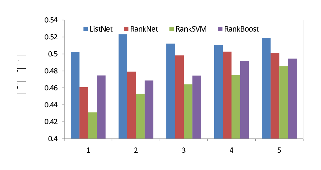
Figure 1 and Table 1 give the results for TREC. We can see that ListNet outperforms the three baseline methods of RankNet, Ranking SVM, and RankBoost in terms of all measures. Especially for NDCG@1 and NDCG@2, ListNet achieves more than 4 point gain, which is about 10% relative improvement.

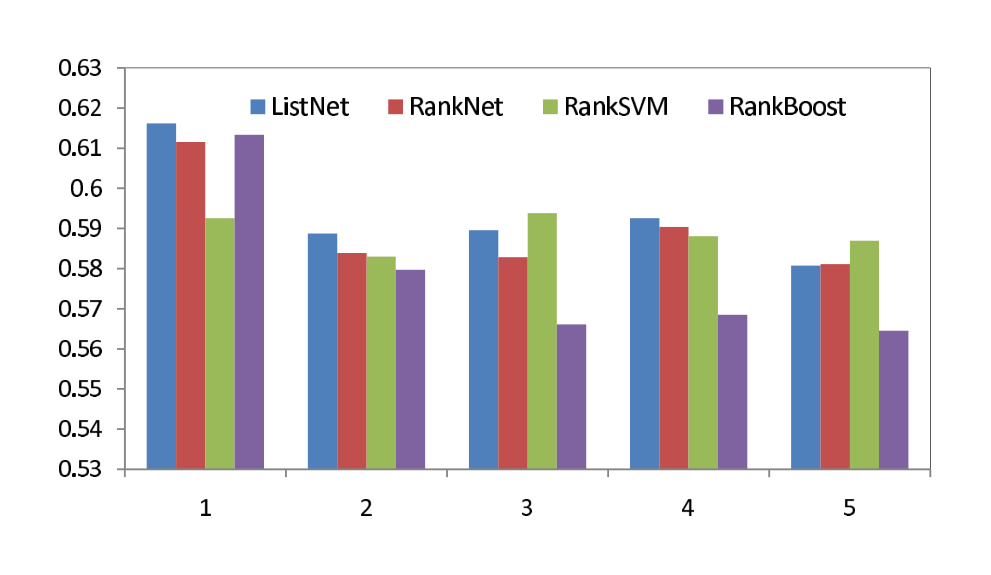
Figure 2 and Table 1 show the results for OHSUMED. Again, ListNet outperforms RankNet and RankBoost in terms of all measures. Moreover, ListNet works better than Ranking SVM in terms of NDCG@1, NDCG@2, NDCG@4 and MAP, with exceptions of NDCG@3 and NDCG@5.

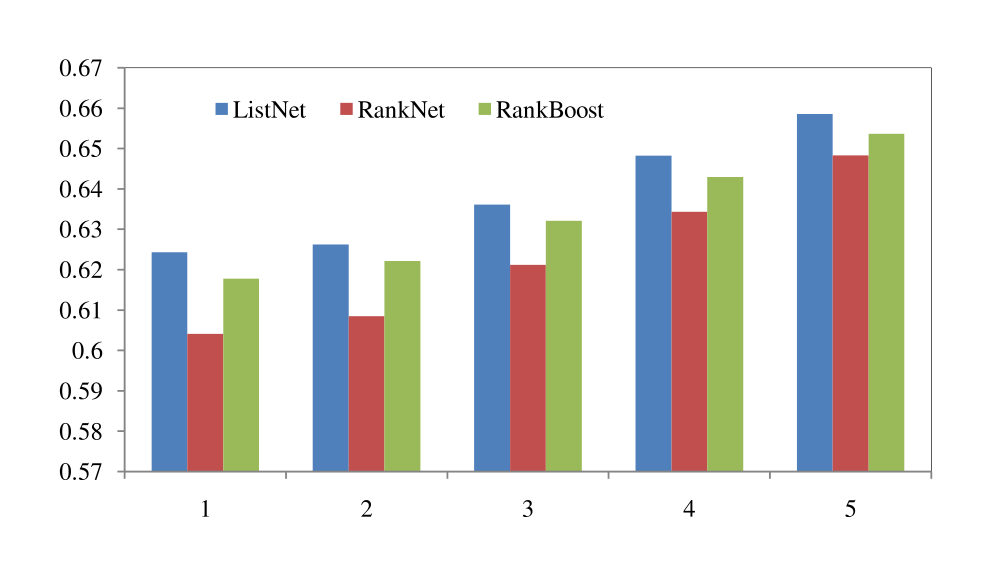
CSearch is a large data set, and thus we did not conduct cross-validation. Instead, we randomly selected one third of the data for training, one third for validation, and the remaining one third for testing. Figure 3 shows the results of ListNet, RankNet and RankBoost. Again, ListNet outperforms RankNet and RankBoost in terms of all measures. Since the size of training data is large, we were not able to run Ranking SVM with the SVMlight tool (Joachims, 1999).

6.3. Discussions

We investigated why the listwise method ListNet can outperform the pairwise methods of RankNet, Ranking SVM, and RankBoost.

As explained in Section 1, for the pairwise approach the number of document pairs varies largely from query to query. As a result, the trained model may be biased toward those queries with more document pairs. We observed the tendencies in all data sets. As example, Table 2 shows the distribution of the number of document pairs per query in OHSUMED. We can see that the distribution is skewed: most queries only have a small number of document pairs (e.g. less than 5,000), while a few queries have a large number of document pairs (e.g. more than 15,000). In the listwise approach the loss function is defined on each query, the problem does not exist. This appears to be one of the reasons for the higher performance by ListNet.

: Table 2: Document-pair number distribution

\begin{tabular}{lc}
\hline
Pair Number & Query Number \\
\hline
<5000 & 61 \\
<10000 & 29 \\
<15000 & 8 \\
<20000 & 6 \\
>=20000 & 2 \\
\hline
\end{tabular}

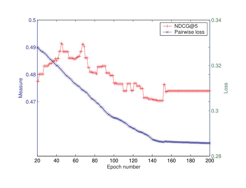
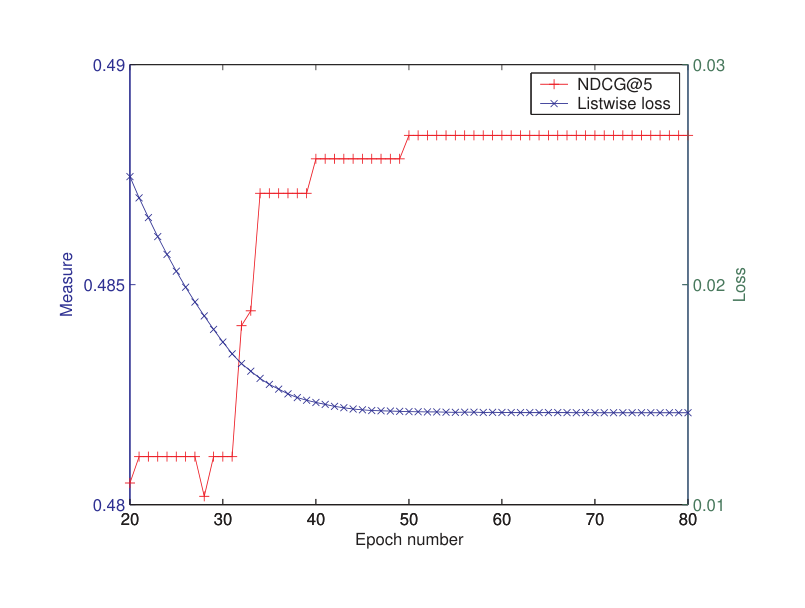
The pairwise approach actually employs a ‘pairwise’ loss function, which might be too loose as an approximation of the performance measures of NDCG and MAP. By contrast, the listwise loss function used in the listwise approach can more properly represent the performance measures. This appears to be another reason that ListNet outperforms RankNet, etc. To verify the correctness of the claim, we further examined the optimization processes of the two methods. We looked at the correlation between the loss functions used by ListNet and RankNet and the measure of NDCG during the learning phase. Note that the major difference between the two methods is the loss function. The results using the TREC data are shown in Figures 4 and 5. From the figures, we can see that the pairwise loss of RankNet does not inversely correlate with NDCG. From iteration 20 to iteration 50, NDCG@5 increases while pairwise loss of RankNet decreases. However, after iteration 60, NDCG@5 starts to drop, although pairwise loss is still decreasing. In contrast, the listwise loss of ListNet completely inversely correlates with NDCG. More specifically, from iteration 20 to iteration 50, listwise loss decreases, NDCG@5 increases accordingly. After iteration 50, listwise loss reaches its limit, while NDCG@5 also converges. Moreover, pairwise loss converges more slowly than listwise loss, which means RankNet needs run more iterations in training than ListNet. Similar trends were observed on the results evaluated in terms of MAP.

We conclude that the listwise approach is more effective than the pairwise approach for learning to rank.

7. Conclusions

Section Summary: The paper introduces a listwise approach to learning to rank, which treats entire lists of objects as training instances rather than individual pairs. It defines a loss function by converting ranking scores into probability distributions using models like permutation probabilities and then applying measures such as cross-entropy. Experiments on three datasets demonstrate that a neural network trained this way outperforms traditional pairwise methods, with suggestions for future improvements in loss functions and evaluation metrics.

In this paper, we have proposed a new approach to learning to rank, referred to as the listwise approach. We argue that it is better to take this approach than the traditional pairwise approach in learning to rank. In the listwise approach, instead of using object pairs as instances, we use list of objects as instances in learning.

The key issue for the listwise approach is to define a listwise loss function. In this paper, we have proposed employing a probabilistic method to solve it. Specifically, we make use of probability models: permutation probability and top one probability to transform ranking scores into probability distributions. We can then view any metric between probability distributions (e.g., Cross Entropy) as the listwise loss function.

We have then developed a learning method based on the approach, using Neural Network and Gradient Descent. Experimental results with three data sets show that the method works better than the existing pairwise methods such as RanNet, Ranking SVM, and RankBoost, suggesting that it is better to take the listwise approach to learning to rank.

Future work includes exploring the performance of other objective function besides cross entropy and the performance of other ranking model instead of linear Neural Network model. We will also investigate the relationship between listwise loss function and performance measures such as NDCG and MAP used in information retrieval.

Acknowledgments

Bin Gao has given many valuable suggestions for this work. We would also like to thanks Kai Yi for his help in our experiments.

References

Section Summary: This section presents a bibliography of academic books and conference papers on information retrieval and ranking methods. The works draw on machine learning techniques, such as support vector machines and boosting algorithms, to improve how search systems order documents by relevance. They also cover evaluation approaches for retrieval results along with foundational ideas from statistics and decision theory.

Baeza-Yates, R., & Ribeiro-Neto, B. (1999). Modern information retrieval. Addison Wesley.

Burges, C., Shaked, T., Renshaw, E., Lazier, A., Deeds, M., Hamilton, N., & Hullender, G. (2005). Learning to rank using gradient descent. Proceedings of ICML 2005 (pp. 89–96).

Cao, Y. B., Xu, J., Liu, T. Y., Li, H., Huang, Y. L., & Hon, H. W. (2006). Adapting ranking SVM to document retrieval. Proceedings of SIGIR 2006 (pp. 186–193).

Cohen, W. W., Schapire, R. E., & Singer, Y. (1998). Learning to order things. Advances in Neural Information Processing Systems. The MIT Press.

Crammer, K., & Singer, Y. (2001). Pranking with ranking. Proceedings of NIPS 2001.

Craswell, N., Hawking, D., Wilkinson, R., & Wu, M. (2003). Overview of the TREC 2003 web track. Proceedings of TREC 2003 (pp. 78–92).

Freund, Y., Iyer, R., Schapire, R. E., & Singer, Y. (1998). An efficient boosting algorithm for combining preferences. Proceedings of ICML 1998 (pp. 170–178).

Herbrich, R., Graepel, T., & Obermayer, K. (1999). Support vector learning for ordinal regression. Proceedings of ICANN 1999 (pp. 97–102).

Hersh, W. R., Buckley, C., Leone, T. J., & Hickam, D. H. (1994). OHSUMED: An interactive retrieval evaluation and new large test collection for research. Proceedings of SIGIR 1994 (pp. 192–201).

Jarvelin, K., & Kekanainen, J. (2000). IR evaluation methods for retrieving highly relevant documents. Proceedings of SIGIR 2000 (pp. 41–48).

Joachims, T. (1999). Making large-scale support vector machine learning practical. Advances in kernel methods: support vector learning, 169–184.

Joachims, T. (2002). Optimizing search engines using clickthrough data. Proceedings of KDD 2002 (pp. 133–142).

Lebanon, G., & Lafferty, J. (2002). Cranking: Combining rankings using conditional probability models on permutations. Proceedings of ICML 2002 (pp. 363–370).

Luce, R. D. (1959). Individual choice behavior. Wiley.

Matveeva, I., Burges, C., Burkard, T., Laucius, A., & Wong, L. (2006). High accuracy retrieval with multiple nested ranker. Proceeings of SIGIR 2006 (pp. 437–444).

Nallapati, R. (2004). Discriminative models for information retrieval. Proceedings of SIGIR 2004 (pp. 64–71).

Plackett, R. L. (1975). The analysis of permutations. Applied Statistics, 24(2), 193–202.

Shashua, A., & Levin, A. (2002). Taxonomy of large margin principle algorithms for ordinal regression problems. Proceedings of NIPS 2002.

Yu, H. (2005). SVM selective sampling for ranking with application to data retrieval. Proceedings of KDD 2005 (pp. 354–363).

Appendix

Section Summary: The appendix presents formal proofs that a defined function P_s over permutations of scored items is a valid probability distribution summing to one, and that it assigns strictly higher probability to orderings in which higher-scoring items appear earlier. It further derives the marginal probability that any given item appears first and shows how the gradient of a loss that uses these probabilities reduces to a simple weighted difference of feature derivatives. These results supply the theoretical and computational basis for optimizing models that rely on the permutation probabilities.

A: Proof of Lemma 2

Proof According to the definition of $\phi(\cdot)$, we have $P_s(\pi) > 0$ for any $\pi \in \Omega_n$. Furthermore,

$ \sum_{\pi \in \Omega_n} P_s(\pi) = \sum_{\pi \in \Omega_n} \prod_{j=1}^n \frac{\phi(s_{\pi(j)})}{\sum_{k=j}^n \phi(s_{\pi(k)})} $

$ = \sum_{\pi(1)=1}^n \sum_{\pi(2)=1, \pi(2) \neq \pi(1)}^n \dots \sum_{\pi(q)=1, \pi(q) \neq \pi(l), \forall l < q}^n \dots \sum_{\pi(n)=1, \pi(n) \neq \pi(l), \forall l < n}^n \prod_{j=1}^n \frac{\phi(s_{\pi(j)})}{\sum_{k=j}^n \phi(s_{\pi(k)})} $

$ = \sum_{\pi(1)=1}^n \frac{\phi(s_{\pi(1)})}{\sum_{k=1}^n \phi(s_{\pi(k)})} \sum_{\pi(2)=1, \pi(2) \neq \pi(1)}^n \frac{\phi(s_{\pi(2)})}{\sum_{k=2}^n \phi(s_{\pi(k)})} \dots \sum_{\pi(q)=1, \pi(q) \neq \pi(l), \forall l < q}^n \frac{\phi(s_{\pi(q)})}{\sum_{k=q}^n \phi(s_{\pi(k)})} \dots \sum_{\pi(n)=1, \pi(n) \neq \pi(l), \forall l < n}^n \frac{\phi(s_{\pi(n)})}{\sum_{k=n}^n \phi(s_{\pi(k)})} $

Since for any $1 \leq q \leq n$,

$ \sum_{\pi(q)=1, \pi(q) \neq \pi(l), \forall l < q}^n \frac{\phi(s_{\pi(q)})}{\sum_{k=q}^n \phi(s_{\pi(k)})} = 1 $

Then, we have, $\sum_{\pi \in \Omega_n} P_s(\pi) = 1$.

Given the two properties above, we conclude that $P_s(\pi), \pi \in \Omega_n$ forms a probability distribution over the set $\Omega_n$. ■

B: Proof of Theorem 3

Proof From Definition 1, we have

$ P_s(\pi) = \prod_{j=1}^n \frac{\phi(s_{\pi(j)})}{\sum_{k=j}^n \phi(s_{\pi(k)})} $

and

$ P_s(\pi') = \prod_{j=1}^n \frac{\phi(s_{\pi'(j)})}{\sum_{k=j}^n \phi(s_{\pi'(k)})} . $

In order to prove $P_s(\pi) > P_s(\pi')$, we need to prove

$ \prod_{j=p}^q \frac{\phi(s_{\pi(j)})}{\sum_{k=j}^n \phi(s_{\pi(k)})} > \prod_{j=p}^q \frac{\phi(s_{\pi'(j)})}{\sum_{k=j}^n \phi(s_{\pi'(k)})} . $

Notice that $\prod_{j=p}^q \phi(s_{\pi(j)}) = \prod_{j=p}^q \phi(s_{\pi'(j)})$. Thus, we need to prove

$ \prod_{j=p}^q \frac{1}{\sum_{k=j}^n \phi(s_{\pi(k)})} > \prod_{j=p}^q \frac{1}{\sum_{k=j}^n \phi(s_{\pi'(k)})} . \tag{4} $

For any $p < j \leq q$, because $s_{\pi(p)} > s_{\pi(q)}$ and $\phi(\cdot)$ is an increasing function, we have $\phi(s_{\pi(p)}) > \phi(s_{\pi(q)})$. Consequently, we have

$ \frac{1}{\sum_{k=j}^n \phi(s_{\pi(k)})} > \frac{1}{\sum_{k=j}^n \phi(s_{\pi'(k)})} . \tag{5} $

With (6) and (5) we can validate that $P_s(\pi) > P_s(\pi')$ holds. ■

C: Proof of Theorem 6

Proof From Definition 2, we have $P_s(j) = \sum_{\pi \in \Omega_n, \pi(1)=j} P_s(\pi) =$

$ = \sum_{\pi \in \Omega_n, \pi(1)=j} \prod_{p=1}^n \frac{\phi(s_{\pi(p)})}{\sum_{k=p}^n \phi(s_{\pi(k)})} $

$ = \sum_{\pi(1)=j, \pi(2)=1, \pi(2) \neq \pi(1)}^n \dots \sum_{\pi(q)=1, \pi(q) \neq \pi(l), \forall l < q}^n \dots \sum_{\pi(n)=1, \pi(n) \neq \pi(l), \forall l < n}^n \prod_{p=1}^n \frac{\phi(s_{\pi(p)})}{\sum_{k=p}^n \phi(s_{\pi(k)})} $

$ = \frac{\phi(s_{\pi(1)})}{\sum_{k=1}^n \phi(s_{\pi(k)})} \sum_{\pi(1)=j, \pi(2)=1, \pi(2) \neq \pi(1)}^n \frac{\phi(s_{\pi(2)})}{\sum_{k=2}^n \phi(s_{\pi(k)})} \dots \sum_{\pi(q)=1, \pi(q) \neq \pi(l), \forall l < m}^n \frac{\phi(s_{\pi(q)})}{\sum_{k=q}^n \phi(s_{\pi(q)})} \dots \sum_{\pi(n)=1, \pi(n) \neq \pi(l), \forall l < n}^n \frac{\phi(s_{\pi(n)})}{\sum_{k=n}^n \phi(s_{\pi(n)})} $

$ = \frac{\phi(s_j)}{\sum_{k=1}^n \phi(s_{\pi(k)})} . \text{ ■} $

D: Derivation of gradient

For Eq. (2)

$ \Delta\omega = \frac{\partial L(y^{(i)}, z^{(i)}(f_\omega))}{\partial \omega} = - \sum_{j=1}^{n^{(i)}} P_{y^{(i)}}(x_j^{(i)}) \frac{\partial \log(P_{z^{(i)}(f_\omega)}(x_j^{(i)}))}{\partial \omega} \tag{6} $

Furthermore, from

$ \log(P_{z^{(i)}(f_\omega)}(x_j^{(i)})) = f_\omega(x_j^{(i)}) - \log \left( \sum_{k=1}^{n^{(i)}} \exp(f_\omega(x_k^{(i)})) \right), $

we have

$ \frac{\partial \log(P_{z^{(i)}(f_\omega)}(x_j^{(i)}))}{\partial \omega} = \frac{\partial f_\omega(x_j^{(i)})}{\partial \omega} - \frac{1}{\sum_{k=1}^{n^{(i)}} \exp(f_\omega(x_k^{(i)}))} \sum_{k=1}^{n^{(i)}} \exp(f_\omega(x_k^{(i)})) \frac{\partial f_\omega(x_k^{(i)})}{\partial \omega} \tag{7} $

Substitute Eq. (7) into Eq. (6) we obtain

$ \Delta\omega = \frac{\partial L(y^{(i)}, z^{(i)}(f_\omega))}{\partial \omega} $

$ = - \sum_{j=1}^{n^{(i)}} P_{y^{(i)}}(x_j^{(i)}) \left( \frac{\partial f_\omega(x_j^{(i)})}{\partial \omega} - \frac{1}{\sum_{k=1}^{n^{(i)}} \exp(f_\omega(x_k^{(i)}))} \sum_{k=1}^{n^{(i)}} \exp(f_\omega(x_k^{(i)})) \frac{\partial f_\omega(x_k^{(i)})}{\partial \omega} \right) $

$ = - \sum_{j=1}^{n^{(i)}} P_{y^{(i)}}(x_j^{(i)}) \frac{\partial f_\omega(x_j^{(i)})}{\partial \omega} + \sum_{j=1}^{n^{(i)}} P_{y^{(i)}}(x_j^{(i)}) \left( \frac{1}{\sum_{k=1}^{n^{(i)}} \exp(f_\omega(x_k^{(i)}))} \sum_{k=1}^{n^{(i)}} \exp(f_\omega(x_k^{(i)})) \frac{\partial f_\omega(x_k^{(i)})}{\partial \omega} \right) $

$ = - \sum_{j=1}^{n^{(i)}} P_{y^{(i)}}(x_j^{(i)}) \frac{\partial f_\omega(x_j^{(i)})}{\partial \omega} + \left( \frac{1}{\sum_{k=1}^{n^{(i)}} \exp(f_\omega(x_k^{(i)}))} \sum_{k=1}^{n^{(i)}} \exp(f_\omega(x_k^{(i)})) \frac{\partial f_\omega(x_k^{(i)})}{\partial \omega} \right) \sum_{j=1}^{n^{(i)}} P_{y^{(i)}}(x_j^{(i)}) \tag{8} $

Since $\sum_{j=1}^{n^{(i)}} P_{y^{(i)}}(x_j^{(i)}) = 1$, we have

$ \Delta\omega = \frac{\partial L(y^{(i)}, z^{(i)}(f_\omega))}{\partial \omega} = - \sum_{j=1}^{n^{(i)}} P_{y^{(i)}}(x_j^{(i)}) \frac{\partial f_\omega(x_j^{(i)})}{\partial \omega} + \frac{1}{\sum_{k=1}^{n^{(i)}} \exp(f_\omega(x_k^{(i)}))} \sum_{k=1}^{n^{(i)}} \exp(f_\omega(x_k^{(i)})) \frac{\partial f_\omega(x_k^{(i)})}{\partial \omega} \tag{9} $

which is equivalent to Eq. (3).