ICLabel: An automated electroencephalographic independent component classifier, dataset, and website

Luca Pion-TonachiniKen Kreutz-DelgadoScott Makeig

article2019NeuroImage2,045 citations

Introduces ICLabel, an automated EEG independent component classifier backed by a crowdsourced dataset of over 200,000 components that achieves state-of-the-art source categorization accuracy ten times faster than previous public methods.

Listen

Electroencephalography provides an accessible, non-invasive method to monitor brain dynamics, but recorded scalp signals invariably mix cortical activity with physiological and non-biological artifacts such as muscle contractions, eye movements, and electrical interference. While independent component analysis successfully separates these mixed recordings into distinct signal sources, the resulting components lack intrinsic labels or ordering. Manually inspecting and categorizing these components is subjective, time-intensive, and impractical for large-scale studies or real-time systems. This article evaluated whether an automated classifier, trained on large-scale crowdsourced annotations, could accurately categorize independent components across multiple categories while maintaining the computational speed required for real-time applications.

The authors developed the ICLabel project, which comprises a massive dataset of over 200,000 independent components drawn from 6,352 recordings, an interactive educational website that collected more than 34,000 component labels from over 250 contributors, and a neural network classifier. Crowdsourced labels were aggregated into probabilistic true-label estimates using an advanced consensus algorithm, yielding nearly 6,000 annotated training examples. The authors trained and cross-validated six candidate artificial neural network architectures and evaluated the final selected models against existing publicly available classifiers on an independent test set of 130 components labeled by six domain experts across diverse experimental conditions.

The evaluation revealed several key findings regarding accuracy, computational efficiency, and architectural choices. First, the final classifier matched or exceeded the accuracy of the best publicly available baseline across standard evaluation metrics, showing particular strength in identifying eye and muscle artifacts. Second, the proposed tool proved roughly ten times faster than the leading automated baseline, processing components in a median time of 170 milliseconds compared to 1.8 seconds. Third, a streamlined variant that omitted autocorrelation features reduced processing time to 120 milliseconds with minimal loss in accuracy. Finally, convolutional neural network architectures that placed double optimization weight on cortical brain components consistently outperformed alternative models, including generative adversarial networks.

These results demonstrate that high-throughput, accurate component classification can be integrated directly into automated preprocessing pipelines and near-real-time brain-computer interfaces without human intervention. The classifier outputs continuous class probabilities across seven categoriesincluding brain, muscle, eye, heart, line noise, and channel noiseallowing practitioners to preserve nuance in ambiguous components or apply custom decision thresholds based on specific experimental needs.

Organizations and researchers processing multichannel electroencephalographic data should integrate the publicly available tool into automated data workflows to reduce manual analysis costs and enhance analytical consistency across studies. Where execution speed is paramount, the streamlined variant offers a practical alternative. Future development should automate periodic model retraining as the crowdsourced database grows and establish recursive feature extraction algorithms to support streaming, causal applications.

Users should exercise caution when applying the model to populations not represented in the training data, such as infant cohorts or clinical populations with significant structural brain trauma, where component properties may differ substantially. In addition, the expert validation set contained limited examples for rare categories like heart-related artifacts and was constrained to a relatively small sample size. Nevertheless, the classifier provides high confidence and strong reliability across standard adult research paradigms.

arXiv: 1901.07915
  • Paper: 1D Convolutional Neural Networks and Applications: A Survey, Serkan Kiranyaz et al. (2019). This survey examines the broader architectural design and engineering applications of 1D convolutional neural networks across biomedical and physical signals, expanding beyond specific EEG multi-component pipelines.
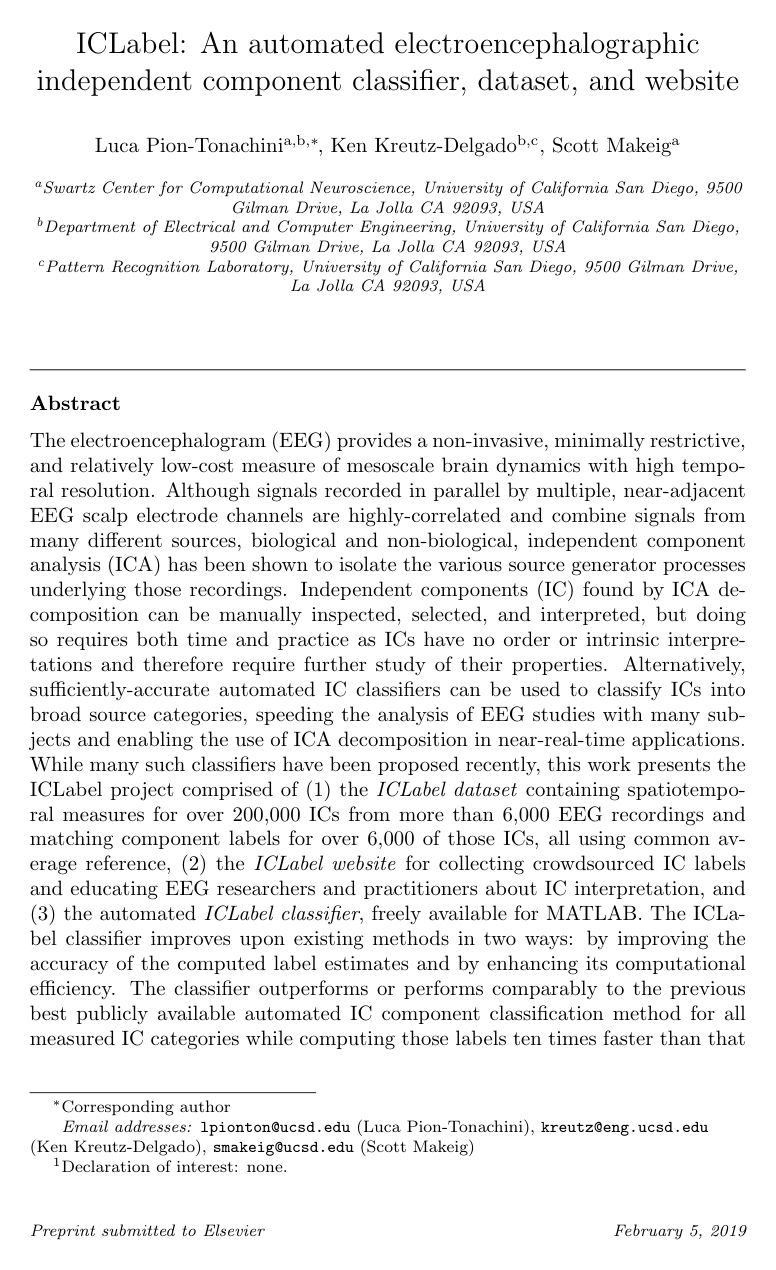
Cover for ICLabel: An automated electroencephalographic independent component classifier, dataset, and website

Abstract

The electroencephalogram (EEG) provides a non-invasive, minimally restrictive, and relatively low cost measure of mesoscale brain dynamics with high temporal resolution. Although signals recorded in parallel by multiple, near-adjacent EEG scalp electrode channels are highly-correlated and combine signals from many different sources, biological and non-biological, independent component analysis (ICA) has been shown to isolate the various source generator processes underlying those recordings. Independent components (IC) found by ICA decomposition can be manually inspected, selected, and interpreted, but doing so requires both time and practice as ICs have no particular order or intrinsic interpretations and therefore require further study of their properties. Alternatively, sufficiently-accurate automated IC classifiers can be used to classify ICs into broad source categories, speeding the analysis of EEG studies with many subjects and enabling the use of ICA decomposition in near-real-time applications. While many such classifiers have been proposed recently, this work presents the ICLabel project comprised of (1) an IC dataset containing spatiotemporal measures for over 200,000 ICs from more than 6,000 EEG recordings, (2) a website for collecting crowdsourced IC labels and educating EEG researchers and practitioners about IC interpretation, and (3) the automated ICLabel classifier. The classifier improves upon existing methods in two ways: by improving the accuracy of the computed label estimates and by enhancing its computational efficiency. The ICLabel classifier outperforms or performs comparably to the previous best publicly available method for all measured IC categories while computing those labels ten times faster than that classifier as shown in a rigorous comparison against all other publicly available EEG IC classifiers.

Table of Contents

  • 1 Introduction and Overview
  • 2 Background
  • 2.1 EEG Component Interpretation
  • 2.2 Prior Methods
  • 2.3 The ICLabel Project
  • 3 Materials and Methods
  • 3.1 ICLabel Dataset and Website
  • 3.1.1 IC Features Descriptions
  • 3.1.2 ICLabel Website and Label Collection
  • 3.1.3 Crowd Labeling
  • 3.2 ICLabel Expert-labeled Test Set
  • 3.3 ICLabel Candidate Classifiers
  • 3.4 Evaluation
  • 4 Results
  • 4.1 ICLabel and Prior Methods
  • 4.2 IC Classification Speed
  • 5 Discussion
  • 5.1 Using Compositional IC Classifications
  • 5.2 Timing
  • 5.3 Differences Between Cross-validated Training Data and Expert-labeled Test Set Results
  • 5.4 Cautions
  • 5.5 An Evolving Classifier
  • 6 Conclusion
  • 7 Acknowledgments
  • References
  • A Evaluation Metrics
  • B Generative Adversarial Networks
  • C ICLabel Candidate Classifier Selection
  • D CL-LDA Details and Hyperparameters
  • E Artificial Neural Network Architecture Details

Knowls

  1. Knowl 1 — ICLabel Multi-Branch Neural Network Architecture

    model/method

    The ICLabel classifier is a multi-branch convolutional neural network (CNN) that estimates class probability distributions across seven independent component (IC) categories from spatiotemporal EEG features:

    1. Scalp Topography Subnetwork: Operates on a 32×32×132 \times 32 \times 1 interpolated scalp projection image, scaled so that its maximum absolute value is 0.990.99. It comprises three 2D convolutional layers with Leaky Rectified Linear Unit (LReLU) activations (leakage parameter 0.20.2):

      • Layer 1: 128 filters, kernel size 4×44 \times 4, stride 2, same padding.
      • Layer 2: 256 filters, kernel size 4×44 \times 4, stride 2, same padding.
      • Layer 3: 512 filters, kernel size 4×44 \times 4, stride 2, same padding.
    2. Power Spectral Density (PSD) Subnetwork: Operates on a 100-element vector representing median log power spectral density from 1 to 100 Hz (computed via Welch's method across time windows, scaled so the maximum absolute value is 0.990.99). It uses three 1D convolutional layers with LReLU:

      • Layer 1: 128 filters, kernel size 3, stride 2, same padding.
      • Layer 2: 256 filters, kernel size 3, stride 2, same padding.
      • Layer 3: 1 filter, kernel size 3, stride 2, same padding.
    3. Autocorrelation Function (ACF) Subnetwork: Operates on a 100-element autocorrelation vector (normalized to a zero-lag value of 0.990.99 before discarding the zero-lag component). It uses three 1D convolutional layers with LReLU:

      • Layer 1: 128 filters, kernel size 3, stride 2, same padding.
      • Layer 2: 256 filters, kernel size 3, stride 2, same padding.
      • Layer 3: 1 filter, kernel size 3, stride 2, same padding.

    The feature outputs of all branches are concatenated and passed into a final layer:

    • Final Classification Layer: 7 filters, kernel size 4×44 \times 4, stride 2, valid padding, followed by a SoftMax activation.

    The model outputs a 7-dimensional compositional probability vector p=[p1,,p7]\mathbf{p} = [p_1, \dots, p_7] such that i=17pi=1\sum_{i=1}^7 p_i = 1. A lightweight variant, ICLabelLite, omits the autocorrelation branch to accelerate feature extraction.

  2. Knowl 2 — EEG Independent Component Seven-Category Taxonomy

    definition

    ICLabel categorizes EEG independent components (ICs) into seven mutually exclusive physiological and artifactual classes:

    • Brain: Locally synchronous cortical field activity generated by one or two bilaterally connected cortical patches. Projections are smoothly varying and dipolar on the scalp, and the power spectrum typically follows an inverse frequency (1/f1/f) trend with elevated power between 5 and 30 Hz.
    • Muscle: Surface electromyographic (EMG) activity from cranial or cervical muscle motor units during contraction or static tension. Characterized by high broadband power at frequencies above 20–30 Hz and spatially localized projections near the scalp boundary.
    • Eye: Electrooculographic activity produced by movements of the corneal-retinal standing potential dipole and eye blinks. Concentrated on frontal electrodes and displaying distinct step or square DC shifts in the component time series.
    • Heart: Far-field electrocardiographic (ECG) volume conduction across the scalp. Displays clear QRS complexes in the time series and a linear diagonal potential gradient from left-posterior to right-anterior.
    • Line Noise: Electrical interference from alternating current power lines (50 Hz or 60 Hz). Shows an extremely sharp, narrow spectral peak at the local power line frequency.
    • Channel Noise: Spatially isolated signal originating from a single electrode, typically caused by high scalp-electrode interface impedance or physical movement of the sensor.
    • Other: Catch-all category containing indeterminate background noise or unresolved mixtures of multiple physical sources that independent component analysis failed to segregate.
  3. Knowl 3 — Loss Weighting, Optimization, and Symmetry Augmentation in ICLabel Training

    model/method

    The ICLabel classifier is trained using weighted cross-entropy optimization and geometric data augmentation:

    • Weighted Cross-Entropy Loss: To prioritize accuracy on neural signals, classification errors on Brain ICs are assigned twice the loss weight (2×2\times) of errors in other classes: L=n=1Ni=1Cwitinlogpin\mathcal{L} = -\sum_{n=1}^N \sum_{i=1}^C w_i t_i^n \log p_i^n where wBrain=2.0w_{\text{Brain}} = 2.0, wiBrain=1.0w_{i \neq \text{Brain}} = 1.0, tint_i^n is the reference compositional label for component nn, and pinp_i^n is the predicted probability for class ii.
    • Optimization: Parameters are updated using the Adam optimizer with learning rate α=0.0003\alpha = 0.0003, decay rates β1=0.5\beta_1 = 0.5 and β2=0.999\beta_2 = 0.999, gradient norm clipping threshold of 20, and mini-batch size of 128 ICs. Batches are constructed using class-balanced random sampling to prevent frequent classes from dominating updates.
    • Convergence and Regularization: Early stopping is evaluated on a holdout validation set over a moving window of 5,000 mini-batches. Gaussian input noise is added to feature representations during training to stabilize convergence.
    • Spatial Symmetry Augmentation: The training data is expanded 4×4\times by applying two spatial transformations to the scalp topographies:
      1. Polarity Inversion: Negating scalp topography values (exploiting the arbitrary sign ambiguity in linear ICA mixing models).
      2. Bilateral Reflection: Horizontally mirroring scalp topography maps (exploiting bilateral anatomical symmetry).
    • Inference Augmentation: During evaluation and deployment, each test IC topography is duplicated across all four polarity and mirror permutations, and the classifier outputs the arithmetic mean of the four predicted probability vectors.
  4. Knowl 4 — Crowd-Label Latent Dirichlet Allocation (CL-LDA) for IC Label Consensus

    algorithm

    To convert redundant, crowdsourced label submissions from web users of varying skill into consensus probabilistic reference labels for training, ICLabel uses Crowd-Label Latent Dirichlet Allocation (CL-LDA).

    For K=7K=7 true classes and J=8J=8 possible user responses (the 7 classes plus an uncertain option ?), each labeler mm is parameterized by a K×JK \times J confusion matrix A(m)\mathbf{A}^{(m)}, where entry Ak,j(m)A_{k,j}^{(m)} is the probability that labeler mm selects response jj given that the component's true class is kk.

    Input: Crowdsourced labels from MM annotators across NN independent components
    Input: Prior Dirichlet parameters for expert and non-expert annotators
    Input: Class prior probabilities πRK\boldsymbol{\pi} \in \mathbb{R}^K
    Output: Compositional consensus label vectors tn[0,1]K\mathbf{t}_n \in [0,1]^K for all n=1,,Nn = 1, \dots, N
    Initialize labeler confusion matrix priors:
      For known experts: set diagonal pseudo-counts to 50.01 and off-diagonals to 0.01
      For unknown annotators: set diagonal pseudo-counts to 1.25 and off-diagonals to 0.25
    Discard all annotators with fewer than 10 total submitted labels
    Run Gibbs sampling for 1000 total epochs:
      For epoch e=1e = 1 to 200 (burn-in period):
        Sample true class assignments for each label instance based on current A(m)\mathbf{A}^{(m)} and π\boldsymbol{\pi}
        Update empirical confusion counts for each annotator
      For epoch e=201e = 201 to 1000 (collection period):
        Sample latent class indicators for each label instance
        Accumulate class assignment counts for each component nn
        Update annotator confusion matrix estimates
    For each component n=1n = 1 to NN:
      Compute the posterior mean compositional label tn=[tn,1,,tn,K]\mathbf{t}_n = [t_{n,1}, \dots, t_{n,K}] by normalizing accumulated class counts, ensuring k=1Ktn,k=1\sum_{k=1}^K t_{n,k} = 1.
  5. Knowl 5 — Soft Confusion Matrices and Soft Operating Characteristics for Compositional Labels

    model/method

    When evaluating classifiers that predict continuous probability vectors p[0,1]C\mathbf{p} \in [0, 1]^C against compositional reference labels t[0,1]C\mathbf{t} \in [0, 1]^C (where i=1Cti=1\sum_{i=1}^C t_i = 1 and i=1Cpi=1\sum_{i=1}^C p_i = 1), soft confusion matrices replace the discrete Boolean AND operator with continuous tt-norms without discretizing or thresholding the labels:

    1. Weak AND (Optimistic Bound): Models maximal possible agreement between reference evidence and prediction: ANDweak(ti,pi)=min(ti,pi)\text{AND}_{\text{weak}}(t_i, p_i) = \min(t_i, p_i)
    2. Product AND (Expected Estimate): Models agreement assuming an independent, uniform distribution of evidence: ANDprod(ti,pi)=tipi\text{AND}_{\text{prod}}(t_i, p_i) = t_i \cdot p_i
    3. Strong AND (Pessimistic Bound): Models worst-case (minimal) overlap between reference evidence and prediction: ANDstrong(ti,pi)=max(ti+pi1,0)\text{AND}_{\text{strong}}(t_i, p_i) = \max(t_i + p_i - 1, 0)

    Applying standard binary performance equations—True Positive Rate (TPR=TPTP+FN\text{TPR} = \frac{\text{TP}}{\text{TP} + \text{FN}}) and False Positive Rate (FPR=FPFP+TN\text{FPR} = \frac{\text{FP}}{\text{FP} + \text{TN}})—to the resulting soft confusion matrices generates three ordered Soft Operating Characteristic (SOC) points (pessimistic, expected, optimistic) in the ROC plane, forming pseudo-confidence intervals on model agreement.

  6. Knowl 6 — Classification Performance Benchmark on Expert-Labeled Test Set

    data/table

    The performance of ICLabel and ICLabelLite was evaluated against competing publicly available IC classifiers on a holdout test set of 130 ICs from 10 recordings across 5 distinct experimental paradigms, with consensus reference labels generated from 6 expert labelers via CL-LDA. Performance is measured across 2-class (Brain vs. Other), 5-class (Brain, Muscle, Eye, Heart, Other), and 7-class evaluations using balanced accuracy (arithmetic mean of within-class recalls; higher is better) and cross-entropy (lower is better):

    Classes Classifier Balanced Accuracy Cross Entropy
    2 ICLabelLite 0.855 0.339
    ICLabel 0.841 0.342
    IC_MARCEF 0.816 0.977
    IC_MARCSF 0.870 0.377
    ADJUST 0.585
    MARA 0.757 0.730
    FASTER 0.578
    SASICA 0.775
    5 ICLabelLite 0.623 0.938
    ICLabel 0.613 0.924
    IC_MARCEF 0.532 2.659
    IC_MARCSF 0.578 0.982
    7 ICLabelLite 0.579 1.287
    ICLabel 0.597 1.251

    While IC_MARC\textsubscript{SF} achieved slightly higher balanced accuracy in the 2-class binary case (0.870 vs. 0.841), ICLabel and ICLabelLite achieved lower cross-entropy and substantially higher balanced accuracy across the 5-class and 7-class evaluations.

  7. Knowl 7 — Computational Speed and Latency of ICLabel Inference

    empirical result

    In single-threaded MATLAB benchmarking on a 2.6 GHz AMD Opteron 6238 processor, ICLabel and ICLabelLite achieved significant speedups over previous component classifiers across all test datasets:

    • ICLabel Execution Time: Median execution time of 170 ms per IC for combined feature extraction and classification. This is 13.0×13.0\times faster than IC_MARC (which required a median of 1.8 s per IC), with per-dataset speedups ranging from 6.7×6.7\times to 64×64\times.
    • ICLabelLite Execution Time: Median execution time of 120 ms per IC (15.5×15.5\times faster than IC_MARC, and 1.36×1.36\times faster than ICLabel due to eliminating autocorrelation computation), with per-dataset speedups up to 88×88\times.
    • Comparison with Alternative Classifiers: Median runtimes were 1.8 s for IC_MARC\textsubscript{EF} and IC_MARC\textsubscript{SF}, 0.5\sim 0.5 s for ADJUST, 0.8\sim 0.8 s for MARA, 0.15\sim 0.15 s for FASTER, and 0.12\sim 0.12 s for SASICA.

    The sub-200 ms latency makes ICLabel suitable for integration into near-real-time streaming pipelines, such as the Real-time EEG Source-mapping Toolbox (REST) using online recursive ICA (ORICA).

  8. Knowl 8 — Ablation Comparison of Candidate Architectures and Feature Sets

    empirical result

    A 3×23 \times 2 factorial evaluation using 10-fold stratified cross-validation on 5,937 labeled ICs from the training set evaluated three architectures—Semi-Supervised Generative Adversarial Network (SSGAN), unweighted CNN, and Brain-loss weighted CNN (wCNN)—across two feature inputs (with and without autocorrelation functions):

    • Network Architecture Comparison: SSGAN candidate models underperformed both CNN and wCNN models across all seven component classes on ROC curves. Weighted CNNs (wCNN) outperformed unweighted CNNs, achieving superior pessimistic and expected Soft Operating Characteristic (SOC) performance across all classes, and highest optimistic performance for Muscle and Eye ICs.
    • Feature Ablation: Including the autocorrelation feature branch alongside scalp topographies and power spectral densities consistently improved classification performance across all categories, with the largest gains observed for Muscle ICs and Other ICs.

    Consequently, the wCNN with autocorrelation was adopted as the standard ICLabel classifier, and the wCNN without autocorrelation was released as ICLabelLite for computation-constrained applications.

  9. Knowl 9 — Optimal Class-Specific Thresholds for Multi-Label Component Detection

    data/table

    When component classification is formulated as multi-label detection (allowing an IC to be assigned zero, one, or multiple independent category tags), decision thresholds θi\theta_i can be selected independently for each category ii by maximizing F1F_1 score or accuracy along the ROC curve:

    Classifier Dataset Metric Brain Muscle Eye Heart Line Noise Channel Noise Other
    ICLabel Train F1F_1 0.40 0.18 0.13 0.33 0.04 0.10 0.12
    ICLabel Train Acc. 0.44 0.18 0.13 0.33 0.04 0.13 0.15
    ICLabel Test F1F_1 0.14 0.29 0.04 0.03 0.84 0.05 0.26
    ICLabel Test Acc. 0.35 0.30 0.04 0.03 0.84 0.05 0.26
    ICLabelLite Train F1F_1 0.39 0.16 0.18 0.44 0.05 0.08 0.11
    ICLabelLite Train Acc. 0.49 0.16 0.18 0.44 0.06 0.08 0.17
    ICLabelLite Test F1F_1 0.05 0.04 0.06 0.10 0.42 0.02 0.29
    ICLabelLite Test Acc. 0.53 0.17 0.06 0.10 0.42 0.15 0.29

    A component with predicted probability vector p=[p1,,p7]\mathbf{p} = [p_1, \dots, p_7] is assigned to category ii if piθip_i \ge \theta_i. This accommodates ambiguous or partially segregated components that contain mixed source characteristics.

  10. Knowl 10 — Generalization Boundaries and Operational Limitations of ICLabel

    limitation

    The performance and applicability of the ICLabel classifier are bounded by specific constraints:

    1. Unrepresented Subject Populations: The training corpus does not include infant EEG data. Because infant brain dynamics differ markedly in spatial projection and spectral composition from adult EEG, the model exhibits degraded accuracy when classifying infant Brain ICs.
    2. Unmodeled Neuropathologies: The dataset does not capture structural brain abnormalities such as brain tumors or severe open head trauma, although data from patients with epilepsy, ADHD, and autism are included.
    3. Electrode Coordinate Approximations: Several datasets in the training corpus relied on standardized template electrode locations rather than subject-specific 3D digitized sensor positions, which introduces spatial distortion into the interpolated scalp topographies.
    4. Feature Non-Causality in Online Mode: The Welch PSD and autocorrelation features used during evaluation are computed over full-length recordings. True real-time online deployment requires substituting non-causal batch calculations with recursive causal estimators to prevent latency delays.

Coverage note — Omitted peripheral website implementation details (Laravel/PHP framework design) and equivalent current dipole (DipFit BEM) extraction details, as dipole fits were excluded from the final neural network feature inputs due to computational overhead.

References

  1. 1.Martın Abadi, Ashish Agarwal, Paul Barham, Eugene Brevdo, Zhifeng Chen, Craig Citro, Greg S. Corrado, Andy Davis, Jeffrey Dean, Matthieu Devin, Sanjay Ghemawat, Ian Goodfellow, Andrew Harp, Geoffrey Irving, Michael Isard, Yangqing Jia, Rafal Jozefowicz, Lukasz Kaiser, Manjunath Kudlur, Josh Levenberg, Dan Mane, Rajat Monga, Sherry Moore, Derek Murray, Chris Olah, Mike Schuster, Jonathon Shlens, Benoit Steiner, Ilya Sutskever, Kunal Talwar, Paul Tucker, Vincent Vanhoucke, Vijay Vasudevan, Fernanda Viegas, Oriol Vinyals, Pete Warden, Martin Wattenberg, Martin Wicke, Yuan Yu, and Xiaoqiang Zheng. TensorFlow: Large-scale machine learning on heterogeneous systems, 2015. URL http://tensorflow.org/. Software available from tensorflow.org.
  2. 2.Geoffray Adde, Maureen Clerc, Olivier Faugeras, Renaud Keriven, Jan Kybic, and Theodore Papadopoulo. Symmetric bem formulation for the m/eeg forward problem. In Chris Taylor and J. Alison Noble, editors, Information Processing in Medical Imaging, pages 524–535, Berlin, Heidelberg, 2003. Springer Berlin Heidelberg.
  3. 3.Shun-ichi Amari, Noboru Murata, Klaus-Robert Muller, Michael Finke, and Howard Hua Yang. Asymptotic statistical theory of overtraining and cross-validation. IEEE Transactions on Neural Networks, 8(5):985–996, Sept 1997. ISSN 1045-9227. doi: 10.1109/72.623200.
  4. 4.Claudia Beleites, Reiner Salzer, and Valter Sergo. Validation of soft classification models using partial class memberships: An extended concept of sensitivity & co. applied to grading of astrocytoma tissues. Chemometrics and Intelligent Laboratory Systems, 122:12 – 22, 2013. ISSN 0169-7439. doi: https://doi.org/10.1016/j.chemolab.2012.12.003. URL http://www.sciencedirect.com/science/article/pii/S0169743912002419.
  5. 5.Anthony J. Bell and Terrence J. Sejnowski. An information-maximization approach to blind separation and blind deconvolution. Neural Computation, 7(6):1129–1159, 1995. doi: 10.1162/neco.1995.7.6.1129. URL https://doi.org/10.1162/neco.1995.7.6.1129.
  6. 6.Nima Bigdely-Shamlo, Tim Mullen, Christian Kothe, Kyung-Min Su, and Kay A. Robbins. The prep pipeline: standardized preprocessing for large-scale eeg analysis. Frontiers in Neuroinformatics, 9:16, 2015. ISSN 1662-5196. doi: 10.3389/fninf.2015.00016. URL https://www.frontiersin.org/article/10.3389/fninf.2015.00016.
  7. 7.Mary A. B. Brazier. A study of the electrical fields at the surface of the head. American Journal of EEG Technology, 6(4):114–128, 1966. doi: 10.1080/00029238.1966.11080676. URL https://doi.org/10.1080/00029238.1966.11080676.
  8. 8.Maximilien Chaumon, Dorothy VM Bishop, and Niko A Busch. A practical guide to the selection of independent components of the electroencephalogram for artifact correction. Journal of neuroscience methods, 250:47–63, 2015.
  9. 9.Zihang Dai, Zhilin Yang, Fan Yang, William W Cohen, and Ruslan R Salakhutdinov. Good semi-supervised learning that requires a bad gan. In Advances in Neural Information Processing Systems, pages 6510–6520, 2017.
  10. 10.Nicolas Della Penna and Mark D Reid. Crowd & prejudice: An impossibility theorem for crowd labelling without a gold standard. arXiv preprint arXiv:1204.3511, 2012.
  11. 11.Arnaud Delorme and Scott Makeig. EEGLAB: an open source toolbox for analysis of single-trial EEG dynamics including independent component analysis. Journal of neuroscience methods, 134(1):9–21, 2004.
  12. 12.Arnaud Delorme, Tim Mullen, Christian Kothe, Zeynep Akalin Acar, Nima Bigdely-Shamlo, Andrey Vankov, and Scott Makeig. EEGLAB, SIFT, NFT, BCILAB, and ERICA: new tools for advanced EEG processing. Computational Intelligence and Neuroscience, 2011:10, 2011.
  13. 13.Arnaud Delorme, Jason Palmer, Julie Onton, Robert Oostenveld, and Scott Makeig. Independent EEG sources are dipolar. PloS One, 7(2):e30135, 2012.
  14. 14.Joseph Dien. Issues in the application of the average reference: Review, critiques, and recommendations. Behavior Research Methods, Instruments, & Computers, 30(1):34–43, 1998.
  15. 15.Laura Frolich, Tobias S. Andersen, and Morten Morup. Classification of independent components of eeg into multiple artifact classes. Psychophysiology, 52(1):32–45, 2015. doi: 10.1111/psyp.12290. URL https://onlinelibrary.wiley.com/doi/abs/10.1111/psyp.12290.
  16. 16.Ian Goodfellow, Jean Pouget-Abadie, Mehdi Mirza, Bing Xu, David Warde-Farley, Sherjil Ozair, Aaron Courville, and Yoshua Bengio. Generative adversarial nets. In Advances in neural information processing systems, pages 2672–2680, 2014.
  17. 17.Frank R Hampel, Elvezio M Ronchetti, Peter J Rousseeuw, and Werner A Stahel. Robust statistics: the approach based on influence functions, volume 196. John Wiley & Sons, 2011.
  18. 18.C.J Henderson, S.R Butler, and A Glass. The localization of equivalent dipoles of eeg sources by the application of electrical field theory. Electroencephalography and Clinical Neurophysiology, 39(2):117 – 130, 1975. ISSN 0013-4694. doi: https://doi.org/10.1016/0013-4694(75)90002-4. URL http://www.sciencedirect.com/science/article/pii/0013469475900024.
  19. 19.Geoffrey Hinton, Oriol Vinyals, and Jeff Dean. Distilling the knowledge in a neural network. arXiv preprint arXiv:1503.02531, 2015.
  20. 20.Sheng-Hsiou Hsu, Tim Mullen, Tzyy-Ping Jung, and Gert Cauwenberghs. Online recursive independent component analysis for real-time source separation of high-density EEG. In Engineering in Medicine and Biology Society (EMBC), 2014 36th Annual International Conference of the IEEE, pages 3845–3848. IEEE, 2014.
  21. 21.Sheng-Hsiou Hsu, Tim R Mullen, Tzyy-Ping Jung, and Gert Cauwenberghs. Real-time adaptive eeg source separation using online recursive independent component analysis. IEEE transactions on neural systems and rehabilitation engineering, 24(3):309–319, 2016.
  22. 22.Sergey Ioffe and Christian Szegedy. Batch normalization: Accelerating deep network training by reducing internal covariate shift. arXiv preprint arXiv:1502.03167, 2015.
  23. 23.Tzyy-Ping Jung, Colin Humphries, Te-Won Lee, Scott Makeig, Martin J McKeown, Vicente Iragui, and Terrence J Sejnowski. Extended ica removes artifacts from electroencephalographic recordings. In Advances in neural information processing systems, pages 894–900, 1998.
  24. 24.Diederik P Kingma and Jimmy Ba. Adam: A method for stochastic optimization. arXiv preprint arXiv:1412.6980, 2014.
  25. 25.Clement Lee and Scott Makeig. get chanlocs: Compute 3-D electrode positions from a 3-D head image. https://sccn.ucsd.edu/wiki/Get_chanlocs, 2018. Accessed: 2019-01-30.
  26. 26.Kimin Lee, Honglak Lee, Kibok Lee, and Jinwoo Shin. Training confidence-calibrated classifiers for detecting out-of-distribution samples. In International Conference on Learning Representations, 2018. URL https://openreview.net/forum?id=ryiAv2xAZ.
  27. 27.Te-Won Lee, Mark Girolami, and Terrence J Sejnowski. Independent component analysis using an extended infomax algorithm for mixed subgaussian and supergaussian sources. Neural computation, 11(2):417–441, 1999.
  28. 28.Andrew L Maas, Awni Y Hannun, and Andrew Y Ng. Rectifier nonlinearities improve neural network acoustic models. In Proc. icml, volume 30, page 3, 2013.
  29. 29.Scott Makeig, Anthony J Bell, Tzyy-Ping Jung, Terrence J Sejnowski, et al. Independent component analysis of electroencephalographic data. Advances in Neural Information Processing Systems, pages 145–151, 1996.
  30. 30.Jaakko Malmivuo and Robert Plonsey. Bioelectromagnetism: Principles and Applications of Bioelectric and Biomagnetic Fields. Oxford University Press, 1995. ISBN 9780195058239. URL https://books.google.com/books?id=H9CFM0TqWwsC.
  31. 31.Peter J Marshall, Yair Bar-Haim, and Nathan A Fox. Development of the eeg from 5 months to 4 years of age. Clinical Neurophysiology, 113(8):1199 – 1208, 2002. ISSN 1388-2457. doi: https://doi.org/10.1016/S1388-2457(02)00163-3. URL http://www.sciencedirect.com/science/article/pii/S1388245702001633.
  32. 32.Andrea Mognon, Jorge Jovicich, Lorenzo Bruzzone, and Marco Buiatti. Adjust: An automatic eeg artifact detector based on the joint use of spatial and temporal features. Psychophysiology, 48(2):229–240, 2011.
  33. 33.Tim Mullen, Christian Kothe, Yu Mike Chi, Alejandro Ojeda, Trevor Kerth, Scott Makeig, Gert Cauwenberghs, and Tzyy-Ping Jung. Real-time modeling and 3d visualization of source dynamics and connectivity using wearable eeg. In 2013 35th Annual International Conference of the IEEE Engineering in Medicine and Biology Society (EMBC), pages 2184–2187, July 2013. doi: 10.1109/EMBC.2013.6609968.
  34. 34.Vinod Nair and Geoffrey E. Hinton. Rectified linear units improve restricted boltzmann machines. In Proceedings of the 27th International Conference on International Conference on Machine Learning, ICML’10, pages 807–814, USA, 2010. Omnipress. ISBN 978-1-60558-907-7. URL http://dl.acm.org/citation.cfm?id=3104322.3104425.
  35. 35.Hugh Nolan, Robert Whelan, and RB Reilly. Faster: fully automated statistical thresholding for eeg artifact rejection. Journal of neuroscience methods, 192 (1):152–162, 2010.
  36. 36.Augustus Odena. Semi-supervised learning with generative adversarial networks. arXiv preprint arXiv:1606.01583, 2016.
  37. 37.Jason A Palmer, Scott Makeig, Kenneth Kreutz-Delgado, and Bhaskar D Rao. Newton method for the ICA mixture model. In ICASSP, pages 1805–1808, 2008.
  38. 38.Luca Pion-Tonachini, Sheng-Hsiou Hsu, Scott Makeig, Tzyy-Ping Jung, and Gert Cauwenberghs. Real-time eeg source-mapping toolbox (rest): Online ica and source localization. In Engineering in Medicine and Biology Society (EMBC), 2015 37th Annual International Conference of the IEEE, pages 4114–4117. IEEE, 2015.
  39. 39.Luca Pion-Tonachini, Scott Makeig, and Ken Kreutz-Delgado. Crowd labeling latent dirichlet allocation. Knowledge and Information Systems, 53(3):749–765, 2017.
  40. 40.Luca Pion-Tonachini, Sheng-Hsiou Hsu, Chi-Yuan Chang, Tzyy-Ping Jung, and Scott Makeig. Online automatic artifact rejection using the real-time eeg source-mapping toolbox (rest). In 2018 40th Annual International Conference of the IEEE Engineering in Medicine and Biology Society (EMBC), pages 106–109. IEEE, 2018.
  41. 41.Lutz Prechelt. Early Stopping — But When?, pages 53–67. Springer Berlin Heidelberg, Berlin, Heidelberg, 2012. ISBN 978-3-642-35289-8. doi: 10.1007/978-3-642-35289-8 5. URL https://doi.org/10.1007/978-3-642-35289-8_5.
  42. 42.Alec Radford, Luke Metz, and Soumith Chintala. Unsupervised representation learning with deep convolutional generative adversarial networks. arXiv preprint arXiv:1511.06434, 2015.
  43. 43.Tim Salimans, Ian Goodfellow, Wojciech Zaremba, Vicki Cheung, Alec Radford, and Xi Chen. Improved techniques for training gans. In Advances in Neural Information Processing Systems, pages 2234–2242, 2016.
  44. 44.Casper Kaae Sonderby, Jose Caballero, Lucas Theis, Wenzhe Shi, and Ferenc Huszar. Amortised MAP inference for image super-resolution. CoRR, abs/1610.04490, 2016. URL http://arxiv.org/abs/1610.04490.
  45. 45.Akash Srivastava, Lazar Valkoz, Chris Russell, Michael U Gutmann, and Charles Sutton. Veegan: Reducing mode collapse in gans using implicit variational learning. In Advances in Neural Information Processing Systems, pages 3308–3318, 2017.
  46. 46.Tatiana A Stroganova, Elena V Orekhova, and Irina N Posikera. Eeg alpha rhythm in infants. Clinical Neurophysiology, 110(6):997 – 1012, 1999. ISSN 1388-2457. doi: https://doi.org/10.1016/S1388-2457(98)00009-1. URL http://www.sciencedirect.com/science/article/pii/S1388245798000091.
  47. 47.Gabriella Tamburro, Patrique Fiedler, David Stone, Jens Haueisen, and Silvia Comani. A new ica-based fingerprint method for the automatic removal of physiological artifacts from eeg recordings. PeerJ, 6:e4380, 2018.
  48. 48.Grigorios Tsoumakas and Ioannis Katakis. Multi-label classification: An overview. International Journal of Data Warehousing and Mining (IJDWM), 3(3):1–13, 2007.
  49. 49.A. Vedaldi and K. Lenc. Matconvnet – convolutional neural networks for matlab. In Proceeding of the ACM Int. Conf. on Multimedia, 2015.
  50. 50.Peter Welch. The use of fast fourier transform for the estimation of power spectra: A method based on time averaging over short, modified periodograms. IEEE Transactions on Audio and Electroacoustics, 15(2):70–73, June 1967. ISSN 0018-9278. doi: 10.1109/TAU.1967.1161901.
  51. 51.Irene Winkler, Stefan Haufe, and Michael Tangermann. Automatic classification of artifactual ica-components for artifact removal in eeg signals. Behavioral and Brain Functions, 7(1):30, 2011.
  52. 52.Irene Winkler, Stephanie Brandl, Franziska Horn, Eric Waldburger, Carsten Allefeld, and Michael Tangermann. Robust artifactual independent component classification for bci practitioners. Journal of neural engineering, 11(3):035013, 2014.

Citation

MLA
Pion-Tonachini, L., et al. “ICLabel: An Automated Electroencephalographic Independent Component Classifier, Dataset, and Website”. NeuroImage, vol. 198, 2019, pp. 181–97, https://doi.org/10.1016/j.neuroimage.2019.05.026.
APA
Pion-Tonachini, L., Kreutz-Delgado, K., & Makeig, S. (2019). ICLabel: An automated electroencephalographic independent component classifier, dataset, and website. NeuroImage, 198, 181–197. https://doi.org/10.1016/j.neuroimage.2019.05.026
Chicago
Pion-Tonachini, L., K. Kreutz-Delgado, and S. Makeig. 2019. “ICLabel: An Automated Electroencephalographic Independent Component Classifier, Dataset, and Website”. NeuroImage 198: 181–97. https://doi.org/10.1016/j.neuroimage.2019.05.026.
Harvard
Pion-Tonachini, L., Kreutz-Delgado, K. and Makeig, S. (2019) “ICLabel: An automated electroencephalographic independent component classifier, dataset, and website”, NeuroImage, 198, pp. 181–197. Available at: https://doi.org/10.1016/j.neuroimage.2019.05.026.
Vancouver
1. Pion-Tonachini L, Kreutz-Delgado K, Makeig S (2019) ICLabel: An automated electroencephalographic independent component classifier, dataset, and website. NeuroImage 198:181–197

BibTeX

@article{Pion_Tonachini_2019, title={ICLabel: An automated electroencephalographic independent component classifier, dataset, and website}, volume={198}, ISSN={1053-8119}, url={http://dx.doi.org/10.1016/j.neuroimage.2019.05.026}, DOI={10.1016/j.neuroimage.2019.05.026}, journal={NeuroImage}, publisher={Elsevier BV}, author={Pion-Tonachini, Luca and Kreutz-Delgado, Ken and Makeig, Scott}, year={2019}, month=Sept, pages={181–197} }
Metadata:Crossref

Access the Paper

This paper is available from its original source. Click below to access the PDF.

Open PDF