Iterative point matching for registration of free-form curves and surfaces

Zhengyou Zhang

article1994IJCV2,548 citations

Develops an efficient iterative point matching algorithm for registering 3D free-form curves and surfaces that accelerates closest-point search via k-D trees and dynamically filters outliers and occlusions using distance statistics for accurate rigid motion estimation.

Listen

The article addresses the challenge of precisely aligning successive 3D visual maps captured by stereo systems on a moving vehicle in rugged terrain. Accurate registration supports vehicle localization, error correction in stereo reconstruction, and construction of a global digital elevation map.

The work set out to develop and test a fast heuristic algorithm that refines an initial rough motion estimate into a precise 3D rigid transformation between two free-form point sets.

The approach iteratively matches each point in the first set to its nearest neighbor in the second set, discards implausible pairings through statistical analysis of distances, and solves for the motion that minimizes the sum of squared distances. The method was evaluated on both synthetic curves with controlled noise levels and real stereo reconstructions of a chair scene and a rock field.

The algorithm converges in 10-40 iterations, reduces average point distance to a few centimeters, and remains accurate even when 10-20 percent of points are outliers or occluded. Rotation and translation errors stay below 5 percent on noisy synthetic data and produce visually consistent alignment on real scenes. A coarse-to-fine sampling strategy cuts runtime by more than half with negligible loss of precision.

These results show that reliable registration of arbitrary shapes is possible without extracting geometric primitives, enabling practical visual navigation and large-scale map building. The technique is faster than global matching methods yet more robust than differential approaches that require very small motion.

Implementations should adopt the non-symmetric matching criterion for speed-critical use and combine the algorithm with a coarse global search when initial motion uncertainty exceeds roughly 20 degrees. Further work is needed to incorporate per-point uncertainty and to segment scenes containing multiple independently moving objects.

The main limitations are dependence on a reasonable starting estimate to avoid local minima, the need to tune one distance threshold to data resolution, and the assumption that the scene is largely static between views. Results are consistent across dozens of trials, yet readers should verify performance on their specific sensor noise characteristics before operational deployment.

INRIA computer vision matching algorithm matching methods iterative point matching free-form curves rigid transformation

Zhang (1994).pdf

Paper: Least-Squares Fitting of Two 3-D Point Sets, K. S. Arun et al. (1987). Arun et al. derive the closed-form singular value decomposition solution for finding the optimal rigid-body transformation between corresponding 3D point sets, which forms the core motion-update step inside the iterative point matching algorithm.
Paper: Least-Squares Estimation of Transformation Parameters Between Two Point Patterns, S. Umeyama (1991). Umeyama provides the robust least-squares formulation for aligning paired point sets while preventing improper reflection matrices, directly underpinning the absolute orientation calculations required at each iteration.
Paper: Comparing Images Using the Hausdorff Distance, Daniel P. Huttenlocher et al. (1993). Huttenlocher et al. formulate shape and point set comparison using nearest-neighbor distance transforms and partial matching criteria that motivate the heuristic correspondence and outlier-rejection strategies used in iterative point registration.
Paper: Surface reconstruction from unorganized points, Hugues Hoppe et al. (1992). Hoppe et al. establish fundamental methods for processing unorganized 3D point clouds without geometric primitives, framing the free-form surface representations that the iterative matching approach is designed to register.
Paper: An Iterative Image Registration Technique with an Application to Stereo Vision, B. D. Lucas et al. (1981). Lucas and Kanade introduce the foundational iterative alignment and coarse-to-fine refinement principles that inspire iterative registration frameworks across visual and spatial representations.

Paper: Point Set Registration: Coherent Point Drift, Andriy Myronenko et al. (2009). Myronenko and Song extend rigid iterative point matching to a probabilistic Expectation-Maximization framework capable of handling both rigid and complex non-rigid point set registration with robust motion coherence.
Paper: A volumetric method for building complex models from range images, B. Curless et al. (1996). Curless and Levoy build directly on multi-view point set and range registration techniques to fuse successively aligned surface scans into seamless, watertight volumetric 3D models.
Paper: Using Spin Images for Efficient Object Recognition in Cluttered 3D Scenes, Andrew E. Johnson et al. (1999). Johnson and Hebert develop local surface descriptors (spin images) that resolve the initial rough alignment bottleneck of iterative point matching by facilitating automatic global matching in cluttered 3D scenes.
Paper: Shape Matching and Object Recognition Using Shape Contexts, Serge Belongie et al. (2002). Belongie et al. generalize iterative point-based matching and assignment to 2D and 3D shape contexts, incorporating non-rigid thin-plate-spline transformations to extend beyond rigid iterative alignment.

Cover for Iterative point matching for registration of free-form curves and surfaces

Abstract

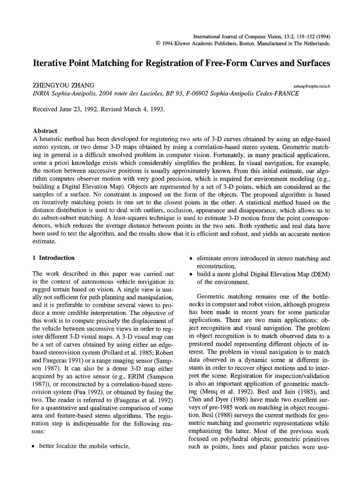
A heuristic method has been developed for registering two sets of 3-D curves obtained by using an edge-based stereo system, or two dense 3-D maps obtained by using a correlation-based stereo system. Geometric matching in general is a difficult unsolved problem in computer vision. Fortunately, in many practical applications, some a priori knowledge exists which considerably simplifies the problem. In visual navigation, for example, the motion between successive positions is usually approximately known. From this initial estimate, our algorithm computes observer motion with very good precision, which is required for environment modeling (e.g., building a Digital Elevation Map). Objects are represented by a set of 3-D points, which are considered as the samples of a surface. No constraint is imposed on the form of the objects. The proposed algorithm is based on iteratively matching points in one set to the closest points in the other. A statistical method based on the distance distribution is used to deal with outliers, occlusion, appearance and disappearance, which allows us to do subset-subset matching. A least-squares technique is used to estimate 3-D motion from the point correspondences, which reduces the average distance between points in the two sets. Both synthetic and real data have been used to test the algorithm, and the results show that it is efficient and robust, and yields an accurate motion estimate.

Topics

computer vision matching algorithm matching methods matching points observer statistical methods stereo-image feature correspondence

Keywords

iterative point matching free-form curves rigid transformation motion estimation Delaunay triangulation quaternion algorithm correlation-based stereovision parametric surface

1 Introduction
2 Problem Statement
3 iterative Pseudo Point Matching Algorithm
3.1 Finding Closest Points
3.2 Pseudo Point Matching
3.3 Updating the Matching
3.4 Computing Motion
3.5 Summary
4 Practical Considerations
4.1 Choice of the Parameter 79
4.2 Choice of the Parameter
4.3 Coarse-to-Fine Strategy
5 Experimental Results with Curves
5.1 A Case Study
5.2 Synthetic Data
5.3 Real Data
6 Experimental Results with Surfaces
6.1A Rock Scene
6.2 A Head Figure
7 Discussions
Z1 About Complexity
7.2 About Convergence
7.3 About Simplifications
7.4 About Sampling
7.5 Uncertainty
7.6 About Large Motion
Z7 Multiple Object Motions
8 Highlights With Respect to Previous Work
9 Conclusions
A Search for Closest Points With k-D Trees
B Motion Computation using Dual Number Quaternions
Acknowledgments
Notes
References
Color Figures

Knowls

Knowl 1 — Iterative Pseudo Point Matching Algorithm for 3-D Shape Registration
algorithm
The iterative pseudo point matching algorithm computes the optimal 3-D rigid transformation $(\mathbf{R}, \mathbf{t})$ —consisting of a rotation matrix $\mathbf{R} \in SO(3)$ and a translation vector $\mathbf{t} \in \mathbb{R}^3$ —between a source point set $\mathcal{X} = \{\mathbf{x}_i\}_{i=1}^m \subset \mathbb{R}^3$ and a target point set $\mathcal{Y} = \{\mathbf{x}'_j\}_{j=1}^n \subset \mathbb{R}^3$ . The method alternates between closest-point pairing, statistical outlier rejection, and closed-form least-squares rigid motion estimation.
Input: Source points $\mathcal{X} = \{\mathbf{x}_i\}_{i=1}^m$ , target points $\mathcal{Y} = \{\mathbf{x}'_j\}_{j=1}^n$ , registration quality parameter $\mathcal{D}$ , orientation threshold $\Theta$
Output: Optimal rigid transformation $(\mathbf{R}, \mathbf{t})$ aligning $\mathcal{X}$ to $\mathcal{Y}$
$D_{\max} \leftarrow 20\mathcal{D}$
$\mathbf{R} \leftarrow \mathbf{I}_{3\times 3}$
$\mathbf{t} \leftarrow \mathbf{0}$
$\mathcal{X}_{\text{current}} \leftarrow \mathcal{X}$
if input represents 3-D curves then
    Compute tangent vectors for all points in $\mathcal{X}$ and $\mathcal{Y}$
Build a 3-D $k$ -d tree representation of $\mathcal{Y}$
repeat
     $\mathcal{M} \leftarrow \emptyset$
    for each point $\mathbf{x}_i \in \mathcal{X}_{\text{current}}$ do
        Find closest point $\mathbf{y}_i \in \mathcal{Y}$ via $k$ -d tree search such that $\|\mathbf{x}_i - \mathbf{y}_i\| \le D_{\max}$
        if $\mathbf{y}_i$ is found then
            if input represents 3-D curves and angle between tangents of $\mathbf{x}_i$ and $\mathbf{y}_i$ exceeds $\Theta$ then
                continue
             $\mathcal{M} \leftarrow \mathcal{M} \cup \{(\mathbf{x}_i, \mathbf{y}_i, \|\mathbf{x}_i - \mathbf{y}_i\|)\}$
    Compute mean $\mu = \frac{1}{|\mathcal{M}|} \sum_{(\mathbf{x}, \mathbf{y}, d) \in \mathcal{M}} d$ and sample standard deviation $\sigma$
    if $\mu < \mathcal{D}$ then
         $D_{\max} \leftarrow \mu + 3\sigma$
    else if $\mu < 3\mathcal{D}$ then
         $D_{\max} \leftarrow \mu + 2\sigma$
    else if $\mu < 6\mathcal{D}$ then
         $D_{\max} \leftarrow \mu + \sigma$
    else
         $D_{\max} \leftarrow \xi$ (histogram valley after the maximal peak)
     $\mathcal{M} \leftarrow \{(\mathbf{x}_i, \mathbf{y}_i, d_i) \in \mathcal{M} \mid d_i \le D_{\max}\}$
    Compute least-squares rigid transformation $(\mathbf{R}_{\text{new}}, \mathbf{t}_{\text{new}})$ from original points $\mathbf{x}_i$ to matched $\mathbf{y}_i$
    Compute rotation axis vector $\mathbf{r}_{\text{new}}$ and translation change $\delta t = \|\mathbf{t}_{\text{new}} - \mathbf{t}\| / \|\mathbf{t}_{\text{new}}\|$ , $\delta r = \|\mathbf{r}_{\text{new}} - \mathbf{r}\| / \|\mathbf{r}_{\text{new}}\|$
     $\mathbf{R} \leftarrow \mathbf{R}_{\text{new}}$
     $\mathbf{t} \leftarrow \mathbf{t}_{\text{new}}$
     $\mathcal{X}_{\text{current}} \leftarrow \{\mathbf{R}\mathbf{x}_i + \mathbf{t} \mid \mathbf{x}_i \in \mathcal{X}\}$
until $(\delta r < 0.01 \text{ and } \delta t < 0.01) \text{ or maximum iterations reached}$
return $(\mathbf{R}, \mathbf{t})$
The computational complexity per iteration is dominated by the closest-point search, which takes expected time $O(m \log n)$ using a 3-D $k$ -d tree. The transformation estimation and point updates run in $O(m)$ time.
Knowl 2 — Dynamic Distance Thresholding for Outlier and Occlusion Rejection
model/method
To handle missing data, occlusions, sensor noise, and appearances/disappearances in subset-subset 3-D shape matching, an adaptive distance threshold $D_{\max}^I$ is dynamically updated at each iteration $I$ based on the sample statistics of matched distances.

Given the set of surviving point pairs $\{(\mathbf{x}_i, \mathbf{y}_i)\}_{i=1}^N$ with Euclidean distances $d_i = \|\mathbf{x}_i - \mathbf{y}_i\|$ , the sample mean $\mu$ and sample standard deviation $\sigma$ are computed as: $\mu = \frac{1}{N} \sum_{i=1}^N d_i, \qquad \sigma = \sqrt{\frac{1}{N} \sum_{i=1}^N (d_i - \mu)^2}$

Let $\mathcal{D}$ be a user-specified reference distance indicating the expected average distance when registration is good (typically set to the average point spacing $\bar{D}$ for curves or twice the spatial resolution for dense range/stereo maps). The threshold $D_{\max}^I$ is set according to the following schedule:
- If $\mu < \mathcal{D}$ (registration is very good): $D_{\max}^I = \mu + 3\sigma$ .
- If $\mathcal{D} \le \mu < 3\mathcal{D}$ (registration is good): $D_{\max}^I = \mu + 2\sigma$ .
- If $3\mathcal{D} \le \mu < 6\mathcal{D}$ (registration is acceptable): $D_{\max}^I = \mu + \sigma$ .
- If $\mu \ge 6\mathcal{D}$ (registration is poor): $D_{\max}^I = \xi$ , where $\xi$ is the distance corresponding to the valley immediately following the highest peak in the histogram of distances, subject to the condition that the number of points at the valley does not exceed $60\%$ of the peak count.
Pairings with $d_i > D_{\max}^I$ are discarded from the subsequent motion computation. In the initial iteration, $D_{\max}^0 = 20\mathcal{D}$ .
Knowl 3 — Closed-Form Rigid Motion Estimation Using Dual Quaternions
model/method
Given $N$ paired 3-D points $\{\mathbf{x}_i\}_{i=1}^N$ and $\{\mathbf{y}_i\}_{i=1}^N$ with associated positive weights $w_i > 0$ , the weighted mean-squares rigid motion objective is: $\mathcal{F}(\mathbf{R}, \mathbf{t}) = \frac{1}{N} \sum_{i=1}^N w_i \|\mathbf{R}\mathbf{x}_i + \mathbf{t} - \mathbf{y}_i\|^2$ where $\mathbf{R} \in SO(3)$ is a rotation matrix and $\mathbf{t} \in \mathbb{R}^3$ is a translation vector.

A rigid displacement is parameterized by a unit dual quaternion $\hat{\mathbf{q}} = \mathbf{q} + \varepsilon \mathbf{s}$ with $\varepsilon^2 = 0$ , where $\mathbf{q} = [\check{\mathbf{q}}^T, q_4]^T \in \mathbb{R}^4$ (with $\check{\mathbf{q}} \in \mathbb{R}^3$ ) and $\mathbf{s} \in \mathbb{R}^4$ satisfy $\mathbf{q}^T \mathbf{q} = 1$ and $\mathbf{q}^T \mathbf{s} = 0$ .

For a quaternion $\mathbf{q} = [\check{\mathbf{q}}^T, q_4]^T$ , define the $4 \times 4$ matrices: $\mathbf{Q}(\mathbf{q}) = \begin{bmatrix} q_4 \mathbf{I}_{3\times 3} + \mathbf{K}(\check{\mathbf{q}}) & \check{\mathbf{q}} \\ -\check{\mathbf{q}}^T & q_4 \end{bmatrix}, \qquad \mathbf{W}(\mathbf{q}) = \begin{bmatrix} q_4 \mathbf{I}_{3\times 3} - \mathbf{K}(\check{\mathbf{q}}) & \check{\mathbf{q}} \\ -\check{\mathbf{q}}^T & q_4 \end{bmatrix}$ where $\mathbf{I}_{3\times 3}$ is the identity matrix and $\mathbf{K}(\check{\mathbf{q}})$ is the $3 \times 3$ skew-symmetric cross-product matrix of $\check{\mathbf{q}}$ . Treating points $\mathbf{x}_i, \mathbf{y}_i$ as pure quaternions $(\mathbf{x}_i, 0)$ and $(\mathbf{y}_i, 0)$ , construct: $W = \sum_{i=1}^N w_i$ $\mathbf{C}_1 = -2 \sum_{i=1}^N w_i \mathbf{Q}(\mathbf{y}_i)^T \mathbf{W}(\mathbf{x}_i) = -2 \sum_{i=1}^N w_i \begin{bmatrix} \mathbf{K}(\mathbf{y}_i)\mathbf{K}(\mathbf{x}_i) + \mathbf{y}_i \mathbf{x}_i^T & -\mathbf{K}(\mathbf{y}_i)\mathbf{x}_i \\ -\mathbf{y}_i^T \mathbf{K}(\mathbf{x}_i) & \mathbf{y}_i^T \mathbf{x}_i \end{bmatrix}$ $\mathbf{C}_2 = 2 \sum_{i=1}^N w_i [\mathbf{W}(\mathbf{x}_i) - \mathbf{Q}(\mathbf{y}_i)] = 2 \sum_{i=1}^N w_i \begin{bmatrix} -\mathbf{K}(\mathbf{x}_i) - \mathbf{K}(\mathbf{y}_i) & \mathbf{x}_i - \mathbf{y}_i \\ -(\mathbf{x}_i - \mathbf{y}_i)^T & 0 \end{bmatrix}$

The rotation quaternion $\mathbf{q}$ is the eigenvector corresponding to the largest eigenvalue of the symmetric $4 \times 4$ matrix: $\mathbf{A} = \frac{1}{2} \left[ \frac{1}{2W} \mathbf{C}_2^T \mathbf{C}_2 - \mathbf{C}_1 - \mathbf{C}_1^T \right]$

The dual part is $\mathbf{s} = -\frac{1}{2W} \mathbf{C}_2 \mathbf{q}$ . The rotation matrix $\mathbf{R}$ and translation vector $\mathbf{t}$ are recovered as: $\mathbf{R} = (q_4^2 - \check{\mathbf{q}}^T\check{\mathbf{q}})\mathbf{I}_{3\times 3} + 2\check{\mathbf{q}}\check{\mathbf{q}}^T + 2q_4 \mathbf{K}(\check{\mathbf{q}})$ $\mathbf{t} = \check{\mathbf{p}}, \quad \text{where } \mathbf{p} = \mathbf{W}(\mathbf{q})^T \mathbf{s}$
Knowl 4 — Recursive Closest-Point Search on 3-D k-D Trees with Adaptive Pruning
algorithm
To accelerate nearest-neighbor queries for $m$ source points against $n$ target points from $O(mn)$ to an expected $O(m \log n)$ , points in the second frame are indexed in a 3-D $k$ -d tree. The tree is built in $O(n \log n)$ time with $O(n)$ storage by recursively partitioning points along planes parallel to the $yz$ -, $xz$ -, and $xy$ -axes passing through median points.

Each node $v$ stores a splitting point $\mathbf{P}(v) \in \mathbb{R}^3$ and a coordinate axis index $t(v) \in \{0, 1, 2\}$ corresponding to $x, y, z$ . The search maintains two global variables: $P$ (the current closest point, initialized to null / $-1$ ) and $D$ (the current search radius bound, initialized to the current iteration threshold $D_{\max}$ ).
Input: Tree node $v$ , query point $\mathbf{x}$ , global variables $P$ and $D$
Output: Closest point $P$ and minimum distance $D$
if $v$ is a leaf node then
    return
$c_1 \leftarrow \mathbf{x}[t(v)]$
$c_2 \leftarrow \mathbf{P}(v)[t(v)]$
if $|c_1 - c_2| \le D$ and $\|\mathbf{x} - \mathbf{P}(v)\| \le D$ then
     $P \leftarrow \mathbf{P}(v)$
    $D \leftarrow \|\mathbf{x} - \mathbf{P}(v)\|
if $c_1 - D < c_2$ then
    SEARCH(leftson( $v$ ), $\mathbf{x}$ )
if $c_2 - D < c_1$ then
    SEARCH(rightson( $v$ ), $\mathbf{x}$ )
Whenever a closer point is found, the global bound $D$ shrinks, which prunes entire branches whose splitting planes lie farther than $D$ from the query point along the splitting dimension.
Knowl 5 — Objective Criteria for Free-Form Curve and Surface Registration
definition
Let $\mathcal{S} = \{\mathbf{x}_i\}_{i=1}^m$ and $\mathcal{S}' = \{\mathbf{x}'_j\}_{j=1}^n$ denote sets of sampled 3-D points from two free-form shapes (curves or surfaces). The symmetric registration criterion optimizes rotation $\mathbf{R} \in SO(3)$ and translation $\mathbf{t} \in \mathbb{R}^3$ by penalizing bidirectional distances: $\mathcal{F}_{\text{sym}}(\mathbf{R}, \mathbf{t}) = \frac{1}{\sum_{i=1}^m p_i} \sum_{i=1}^m p_i d^2(\mathbf{R}\mathbf{x}_i + \mathbf{t}, \mathcal{S}') + \frac{1}{\sum_{j=1}^n q_j} \sum_{j=1}^n q_j d^2(\mathbf{R}^T \mathbf{x}'_j - \mathbf{R}^T \mathbf{t}, \mathcal{S})$ where $d(\mathbf{x}, \mathcal{S}') = \min_{j \in \{1,\dots,n\}} \|\mathbf{x} - \mathbf{x}'_j\|$ , and $p_i, q_j \in \{0, 1\}$ are binary match indicators ( $p_i = 1$ if $\mathbf{x}_i$ has a valid correspondence on $\mathcal{S}'$ , and $0$ otherwise).

The non-symmetric registration criterion restricts the objective to a one-way mapping from the first frame to the second frame to reduce computational cost: $\mathcal{F}(\mathbf{R}, \mathbf{t}) = \frac{1}{\sum_{i=1}^m p_i} \sum_{i=1}^m p_i d^2(\mathbf{R}\mathbf{x}_i + \mathbf{t}, \mathcal{S}')$ In the noise-free case with complete overlap, both objective criteria evaluate to zero at perfect alignment.
Knowl 6 — Convergence Bounds and Non-Monotonicity in Iterative Pseudo Point Matching
theoretical result
In the iterative pseudo point matching framework with dynamic outlier rejection, the sequence of mean squared errors is upper-bounded by the distance thresholds, but the objective value does not necessarily decrease strictly monotonically from iteration to iteration.

At iteration $I$ , given transformation $(\mathbf{R}^{I-1}, \mathbf{t}^{I-1})$ :
1. Closest-point matching retains points satisfying distance bound $D_{\max}^{I-1}$ , producing mean squared error: $d_{\text{closest}}^I = \frac{1}{\sum p_i} \sum_{i=1}^m p_i \|\mathbf{R}^{I-1}\mathbf{x}_i + \mathbf{t}^{I-1} - \mathbf{y}_i\|^2 \le D_{\max}^{I-1}$
2. Discarding pairings with distances exceeding the updated threshold $D_{\max}^I$ yields: $d_{\text{update}}^I \le d_{\text{closest}}^I \le D_{\max}^{I-1} \quad \text{and} \quad d_{\text{update}}^I \le D_{\max}^I$
3. The least-squares transformation $(\mathbf{R}^I, \mathbf{t}^I)$ guarantees: $d_{\text{lsq}}^I = \frac{1}{\sum p_i} \sum_{i=1}^m p_i \|\mathbf{R}^I\mathbf{x}_i + \mathbf{t}^I - \mathbf{y}_i\|^2 \le d_{\text{update}}^I \le \min(d_{\text{closest}}^I, D_{\max}^I)$
However, $d_{\text{closest}}^{I+1} \le d_{\text{lsq}}^I$ is not guaranteed in general. The set of points matching under $D_{\max}^I$ at iteration $I+1$ contains both the points in $d_{\text{lsq}}^I$ (whose individual errors strictly decrease) and newly admitted points previously rejected at iteration $I$ whose distances now fall below $D_{\max}^I$ . Adding these newly matched points can increase the average distance. Enforcing $D_{\max}^I \le D_{\max}^{I-1}$ ensures that the global bounding envelope decreases monotonically.
Knowl 7 — Coarse-to-Fine Subsampling Strategy for Accelerated Registration
model/method
Because the closest-point search runtime is proportional to the number of query points $m$ in the source frame, and because convergence toward the basin of attraction of a local minimum occurs rapidly in the early iterations, a coarse-to-fine subsampling strategy is used to accelerate the registration process.

During the initial iterations (e.g., iterations 1 to 5), only a uniform subset of points from the first frame (such as 1 out of every 5 or 1 out of every 10 sample points) is matched against the target $k$ -d tree. Once the coarse iterations bring the shapes into close alignment, all $m$ sample points are used in subsequent iterations (e.g., iterations 6 to 15) for precise motion refinement.

On synthetic 3-D curve benchmarks with zero-mean Gaussian coordinate noise (standard deviation $\sigma = 3$ ), using 1-in-5 subsampling for the first 5 iterations followed by 10 full iterations achieves comparable accuracy (rotation error $4.56\%$ , translation error $4.29\%$ ) to running 15 iterations with all points (rotation error $4.68\%$ , translation error $4.14\%$ ), while reducing total computation time from 7.49 seconds to 3.39 seconds (a speedup of over $2\times$ ).
Knowl 8 — Orientation Consistency Pruning for Point Matching
model/method
To discard false nearest-neighbor pairings and expand the convergence basin under larger initial displacements, candidate point matches are pruned using local orientation vectors (tangent vectors for 3-D curves or surface normal vectors for surfaces).

For a point $\mathbf{x}_i$ with unit orientation vector $\mathbf{v}_{\mathbf{x}_i}$ in the first frame and candidate closest point $\mathbf{y}_j$ with unit orientation vector $\mathbf{v}_{\mathbf{y}_j}$ in the second frame, the angular difference cannot exceed the rigid rotation angle between the two frames. Matches are retained only if: $\arccos(\mathbf{v}_{\mathbf{x}_i} \cdot \mathbf{v}_{\mathbf{y}_j}) \le \Theta$ where $\Theta$ is a fixed upper bound on expected rotation between successive frames.

For 3-D space curves, approximate unit tangents are computed at each point from the vector connecting neighboring points along the chained curve. To account for finite-difference tangent estimation errors in noisy data, the threshold is set to $\Theta = 60^\circ$ . Any match whose orientation difference exceeds $\Theta$ is discarded ( $p_i = 0$ ).
Knowl 9 — Uncertainty Incorporation via Weighted Least-Squares and Mahalanobis Distance
model/method
When 3-D points reconstructed from sensors (such as stereo vision) have anisotropic Gaussian position uncertainties characterized by $3 \times 3$ covariance matrices $\mathbf{\Lambda}_{\mathbf{x}_i}$ and $\mathbf{\Lambda}_{\mathbf{y}_i}$ , point matching and motion estimation can incorporate uncertainty directly.

In motion estimation, each correspondence is assigned a scalar weight $w_i$ inversely proportional to the trace of the total error covariance matrix $\mathbf{\Lambda}_i = \mathbf{R}\mathbf{\Lambda}_{\mathbf{x}_i}\mathbf{R}^T + \mathbf{\Lambda}_{\mathbf{y}_i}$ : $w_i = \frac{1}{\operatorname{tr}(\mathbf{\Lambda}_i)} \approx \frac{1}{\operatorname{tr}(\mathbf{\Lambda}_{\mathbf{x}_i}) + \operatorname{tr}(\mathbf{\Lambda}_{\mathbf{y}_i})}$

In candidate matching and outlier pruning, the Euclidean distance is replaced by the squared Mahalanobis distance: $d_i^M = (f(\mathbf{d})\mathbf{x}_i + g(\mathbf{d}) - \mathbf{y}_i)^T \mathbf{\Lambda}_i^{-1} (f(\mathbf{d})\mathbf{x}_i + g(\mathbf{d}) - \mathbf{y}_i)$ where $\mathbf{d} = [\mathbf{r}^T, \mathbf{t}^T]^T$ is the motion parameter vector with covariance $\mathbf{\Lambda}_{\mathbf{d}}$ , $\mathbf{R} = f(\mathbf{d})$ , $\mathbf{t} = g(\mathbf{d})$ , and $\mathbf{\Lambda}_i = f(\mathbf{d})\mathbf{\Lambda}_{\mathbf{x}_i}f(\mathbf{d})^T + \mathbf{\Lambda}_{\mathbf{y}_i} + \mathbf{J}_{\mathbf{d}}\mathbf{\Lambda}_{\mathbf{d}}\mathbf{J}_{\mathbf{d}}^T$ (with Jacobian $\mathbf{J}_{\mathbf{d}} = \frac{\partial [f(\mathbf{d})\mathbf{x}_i + g(\mathbf{d})]}{\partial \mathbf{d}}$ ).

Because $d_i^M$ follows a $\chi^2$ distribution with 3 degrees of freedom, pairings are accepted only if $d_i^M \le \varepsilon$ , where $\varepsilon = 7.81$ corresponds to an $89\%$ confidence threshold.

Knowl 10 — Performance Comparison Between Symmetric and Non-Symmetric Matching Criteria

data/table

The non-symmetric matching criterion (one-way matching) and symmetric criterion (two-way matching) were evaluated on a synthetic 3-D space curve $\mathbf{x}(u) = [u^2, 5u \sin(u) + 10u \cos(1.5u), 0]^T$ sampled into 200 points, transformed by ground-truth rotation $\mathbf{r} = [0.02, 0.25, -0.15]^T$ (in radians) and translation $\mathbf{t} = [40.0, 120.0, -50.0]^T$ (in centimeters), with zero-mean Gaussian noise of standard deviation $\sigma \in \{0, 2, 4, 6, 8, 10\}$ added to each coordinate. Metrics are averaged over 10 independent trials after 10 iterations.

Relative rotation and translation errors are defined as $e_r = \frac{\|\mathbf{r} - \hat{\mathbf{r}}\|}{\|\mathbf{r}\|} \times 100\%$ and $e_t = \frac{\|\mathbf{t} - \hat{\mathbf{t}}\|}{\|\mathbf{t}\|} \times 100\%$ .

Noise Std Dev ( $\sigma$ )	0		2		4		6		8
Matching Criterion	Non-sym	Sym	Non-sym	Sym	Non-sym	Sym	Non-sym	Sym	Non-sym	Sym
Rotation Error (%)	1.81	0.12	4.36	2.68	4.60	3.63	7.56	6.40	11.35	8.52
Translation Error (%)	8.22	5.83	7.38	6.35	8.56	7.32	7.61	6.42	7.36	7.08
Execution Time (s)	5.04	10.04	5.32	10.80	6.10	12.54	7.64	15.88	8.18	16.74

The symmetric matching criterion produces lower rotation and translation errors across all noise levels because both point sets contribute equally to the registration objective. However, the symmetric criterion doubles the execution time because closest points and $k$ -d trees must be evaluated in both directions.

Coverage note — Qualitative descriptions and visual figures of real-data experiments (the trinocular stereo chair scene, correlation stereo rock scene, and range image head registration) were omitted as standalone knowls because they demonstrate the execution of the general algorithms already fully captured in the extracted knowls.

References

1.Arun, K., Huang, T. and Blostein, S.: 1987, Least-squares fitting of two 3-D point sets, IEEE Trans. PAMI 9(5), 698-700.
2.Ayache, N. and Faugeras, O. D.: 1989, Maintaining Representations of the Environment of a Mobile Robot, IEEE Trans. RA 5(6), 804-819.
3.Besl, P. and Jain, R.: 1985, Three-dimensional object recognition, ACM Computing Surveys 17(1), 75-145.
4.Besl, P. J.: 1988, Geometric modeling and computer vision, Proc. IEEE 76(8), 936-958.
5.Besl, P. J. and McKay, N. D.: 1992, A method for registration of 3-D shapes, IEEE Trans. PAMI 14(2), 239-256.
6.Blostein, S. and Huang, T.: 1987, Error analysis in stereo determination of a 3-D point position, IEEE Trans. PAMI 9(6), 752-765.
7.Bolles, R. and Cain, R.: 1982, Recognizing and locating partially visible objects, the local-feature-focus method, Int'l J. Robotics Res. 1(3), 57-82.
8.Brockett, R.: 1989, Least squares matching problems, Linear Algebra and Its Applications 122/123/124, 761-777.
9.Champleboux, G., Lavallée, S., Szeliski, R. and Brunie, L.: 1992, From accurate range imaging sensor calibration to accurate model-based 3-D object localization, Proc. IEEE Conf. Comput. Vision Pattern Recog., Champaign, Illinois, pp. 83-89.
10.Chen, X.: 1992, Vision-Based Geometric Modeling, Ph.D. dissertation, Ecole Nationale Supérieure des Télécommunications, Paris, France.
11.Chen, Y. and Medioni, G.: 1992, Object modelling by registration of multiple range images, Image and Vision Computing 10(3), 145-155.
12.Chin, R. and Dyer, C.: 1986, Model-based recognition in robot vision, ACM Computing Surveys 18(1), 67-108.
13.Faugeras, O. and Hebert, M.: 1986, The representation, recognition, and locating of 3D shapes from range data, Int'l J. Robotics Res. 5(3), 27-52.
14.Faugeras, O. D., Lebras-Mehlman, E. and Boissonnat, J.: 1990, Representing Stereo data with the Delaunay Triangulation, Artif. Intell.
15.Faugeras, O., Fua, P., Hotz, B., Ma, R., Robert, L., Thonnat, M. and Zhang, Z.: 1992, Quantitative and qualitative comparison of some area and feature-based stereo algorithms, in W. Förstner and S. Ruwiedel (eds), Robust Computer Vision: Quality of Vision Algorithms, Wichmann, Karlsruhe, Germany, pp. 1-26.
16.Fua, P.: 1992, A parallel stereo algorithm that produces dense depth maps and preserves image features, Machine Vision and Applications. Accepted for publication.
17.Gennery, D. B.: 1989, Visual terrain matching for a Mars rover, Proc. IEEE Conf. Comput. Vision Pattern Recog., San Diego, CA, pp. 483-491.
18.Goldgof, D. B., Huang, T. S. and Lee, H.: 1988, Feature extraction and terrain matching, Proc. IEEE Conf. Comput. Vision Pattern Recog., Ann Arbor, Michigan, pp. 899-904.
19.Grimson, W.: 1985, Computational experiments with a feature based stereo algorithm, IEEE Trans. PAMI 7(1), 17-34.
20.Gueziec, A. and Ayache, N.: 1992, Smoothing and matching of 3-D space curves, Proc. Second European Conf. Comput. Vision, Santa Margharita Ligure, Italy, pp. 620-629.
21.Haralick, R. et al.: 1989, Pose estimation from corresponding point data, IEEE Trans. SMC 19(6), 1426-1446.
22.Hebert, M., Caillas, C., Krotkov, E., Kweon, I. S. and Kanade, T.: 1989, Terrain mapping for a roving planetary explorer, Proc. Int'l Conf. Robotics Automation, pp. 997-1002.
23.Horn, B.: 1987, Closed-form solution of absolute orientation using unit quaternions, Journal of the Optical Society of America A 7, 629-642.
24.Horn, B. and Harris, J.: 1991, Rigid body motion from range image sequences, CVGIP: Image Understanding 53(1), 1-13.
25.Kamgar-Parsi, B., Jones, J. L. and Rosenfeld, A.: 1991, Registration of multiple overlapping range images: Scenes without distinctive features, IEEE Trans. PAMI 13(9), 857-871.
26.Kehtarnavaz, N. and Mohan, S.: 1989, A framework for estimation of motion parameters from range images, Comput. Vision, Graphics Image Process. 45, 88-105.
27.Kriegman, D., Triendl, E. and Binford, T.: 1989, Stereo vision and navigation in buildings for mobile robots, IEEE Trans. RA 5(6), 792-803.
28.Kweon, I. and Kanade, T.: 1992, High-resolution terrain map from multiple sensor data, IEEE Trans. PAMI 14(2), 278-292.
29.Liang, P. and Todhunter, J. S.: 1990, Representation and recognition of surface shapes in range images: A differential geometry approach, Comput. Vision, Graphics Image Process. 52, 78-109.
30.Matthies, L. and Shafer, S. A.: 1987, Error modeling in stereo navigation, IEEE J. RA 3(3), 239-248.
31.Mayhew, J. E. W. and Frisby, J. P.: 1981, Psychophysical and computational studies towards a theory of human stereopsis, Artif. Intell. 17, 349-385.
32.Menq, C.-H., Yau, H.-T. and Lai, G.-Y.: 1992, Automated precision measurement of surface profile in CAD-directed inspection, IEEE Trans. RA 8(2), 268-278.
33.Milios, E. E.: 1989, Shape matching using curvature processes, Comput. Vision, Graphics Image Process. 47, 203-226.
34.Navab, N. and Zhang, Z.: 1992, From multiple objects motion analysis to behavior-based object recognition, Proc. ECAI 92, Vienna, Austria, pp. 790-794.
35.Pavlidis, T.: 1980, Algorithms for shape analysis of contours and waveforms, IEEE Trans. PAMI 2(4), 301-312.
36.Pollard, S., Mayhew, J. and Frisby, J.: 1985, PMF: A stereo correspondence algorithm using a disparity gradient limit, Perception 14, 449-470.
37.Preparata, F. and Shamos, M.: 1986, Computational Geometry, An Introduction, Springer, Berlin, Heidelberg, New-York.
38.Radack, G. M. and Badler, N. I.: 1989, Local matching of surfaces using a boundary-centered radial decomposition, Comput. Vision, Graphics Image Process. 45, 380-396.
39.Robert, L. and Faugeras, O.: 1991, Curve-based stereo: Figural continuity and curvature, Proc. IEEE Conf. Comput. Vision Pattern Recog., Maui, Hawaii, pp. 57-62.
40.Rodríguez, J. J. and Aggarwal, J. K.: 1989, Navigation using image sequence analysis and 3-D terrain matching, Proc. Workshop on Interpretation of 3D Scenes, Austin, TX, pp. 200-207.
41.Safaee-Rad, R., Tchoukanov, I., Benhabib, B. and Smith, K. C.: 1991, Accurate parameter estimation of quadratic curves from grey-level images, CVGIP: Image Understanding 54(2), 259-274.
42.Sampson, R. E.: 1987, 3D range sensor-phase shift detection, Computer 20, 23-24.
43.Schwartz, J. T. and Sharir, M.: 1987, Identification of partially obscured objects in two and three dimensions by matching noisy characteristic curves, Int'l J. Robotics Res. 6(2), 29-44.
44.Szeliski, R.: 1988, Estimating motion from sparse range data without correspondence, Proc. Second Int'l Conf. Comput. Vision, IEEE, Tampa, FL, pp. 207-216.
45.Szeliski, R.: 1990, Bayesian modeling of uncertainty in low-level vision, Int'l J. Comput. Vision 5(3), 271-301.
46.Taubin, G.: 1991, Estimation of planar curves, surfaces, and non-planar space curves defined by implicit equations with applications to edge and range image segmentation, IEEE Trans. PAMI 13(11), 1115-1138.
47.Walker, M. W., Shao, L. and Volz, R. A.: 1991, Estimating 3-D location parameters using dual number quaternions, CVGIP: Image Understanding 54(3), 358-367.
48.Walters, D.: 1987, Selection of image primitives for general-purpose visual processing, Comput. Vision, Graphics Image Process. 37(3), 261-298.
49.Wolfson, H.: 1990, On curve matching, IEEE Trans. PAMI 12(5), 483-489.
50.Zhang, Z.: 1991, Recalage de deux cartes de profondeur denses: L'état de l'art, Rapport VAP de la phase 4, CNES, Toulouse, France.
51.Zhang, Z.: 1992a, Iterative point matching for registration of free-form curves, Research Report 1658, INRIA Sophia-Antipolis.
52.Zhang, Z.: 1992b, On local matching of free-form curves, Proc. British Machine Vision Conf., University of Leeds, UK, pp. 347-356.
53.Zhang, Z. and Faugeras, O.: 1991, Determining motion from 3D line segments: A comparative study, Image and Vision Computing 9(1), 10-19.
54.Zhang, Z. and Faugeras, O.: 1992a, 3D Dynamic Scene Analysis: A Stereo Based Approach, Springer, Berlin, Heidelberg.
55.Zhang, Z. and Faugeras, O.: 1992b, Three-dimensional motion computation and object segmentation in a long sequence of stereo frames, Int'l J. Comput. Vision 7(3), 211-241.
56.Zhang, Z., Faugeras, O. and Ayache, N.: 1988, Analysis of a sequence of stereo scenes containing multiple moving objects using rigidity constraints, Proc. Second Int'l Conf. Comput. Vision, Tampa, FL, pp. 177-186. Also as a chapter in R. Kasturi and R.C. Jain (eds), Computer Vision: Principles, IEEE computer society press, 1991.

Citation

MLA

Zhang, Z. “Iterative Point Matching for Registration of Free-form Curves and Surfaces”. International Journal of Computer Vision, vol. 13, no. 2, 1994, pp. 119–52, https://doi.org/10.1007/BF01427149.

APA

Zhang, Z. (1994). Iterative point matching for registration of free-form curves and surfaces. International Journal of Computer Vision, 13(2), 119–152. https://doi.org/10.1007/BF01427149

Chicago

Zhang, Z. 1994. “Iterative Point Matching for Registration of Free-form Curves and Surfaces”. International Journal of Computer Vision 13 (2): 119–52. https://doi.org/10.1007/BF01427149.

Harvard

Zhang, Z. (1994) “Iterative point matching for registration of free-form curves and surfaces”, International Journal of Computer Vision, 13(2), pp. 119–152. Available at: https://doi.org/10.1007/BF01427149.

Vancouver

1. Zhang Z (1994) Iterative point matching for registration of free-form curves and surfaces. International Journal of Computer Vision 13:119–152

BibTeX

@article{Zhang_1994, title={Iterative point matching for registration of free-form curves and surfaces}, volume={13}, ISSN={1573-1405}, url={http://dx.doi.org/10.1007/BF01427149}, DOI={10.1007/bf01427149}, number={2}, journal={International Journal of Computer Vision}, publisher={Springer Science and Business Media LLC}, author={Zhang, Zhengyou}, year={1994}, month=Oct, pages={119–152} }

Metadata:Crossref

Access the Paper

This paper is available from its original source. Click below to access the PDF.

Open PDF

Iterative point matching for registration of free-form curves and surfaces

Abstract

Topics

Keywords

Table of Contents

Knowls

Knowl 1 — Iterative Pseudo Point Matching Algorithm for 3-D Shape Registration

Knowl 2 — Dynamic Distance Thresholding for Outlier and Occlusion Rejection

Knowl 3 — Closed-Form Rigid Motion Estimation Using Dual Quaternions

Knowl 4 — Recursive Closest-Point Search on 3-D k-D Trees with Adaptive Pruning

Knowl 5 — Objective Criteria for Free-Form Curve and Surface Registration

Knowl 6 — Convergence Bounds and Non-Monotonicity in Iterative Pseudo Point Matching

Knowl 7 — Coarse-to-Fine Subsampling Strategy for Accelerated Registration

Knowl 8 — Orientation Consistency Pruning for Point Matching

Knowl 9 — Uncertainty Incorporation via Weighted Least-Squares and Mahalanobis Distance

Knowl 10 — Performance Comparison Between Symmetric and Non-Symmetric Matching Criteria

References

Citation

BibTeX

Access the Paper