Sinkhorn Distances: Lightspeed Computation of Optimal Transportation Distances

MARCO CUTURI

Abstract

Optimal transportation distances are a fundamental family of parameterized distances for histograms. Despite their appealing theoretical properties, excellent performance in retrieval tasks and intuitive formulation, their computation involves the resolution of a linear program whose cost is prohibitive whenever the histograms' dimension exceeds a few hundreds. We propose in this work a new family of optimal transportation distances that look at transportation problems from a maximum-entropy perspective. We smooth the classical optimal transportation problem with an entropic regularization term, and show that the resulting optimum is also a distance which can be computed through Sinkhorn-Knopp's matrix scaling algorithm at a speed that is several orders of magnitude faster than that of transportation solvers. We also report improved performance over classical optimal transportation distances on the MNIST benchmark problem.

Executive Summary: Comparing probability distributions and histogram data is a foundational task in modern data analysis and machine learning, particularly in computer vision. Optimal transportation distances, commonly referred to as Earth Mover's Distances, offer powerful theoretical properties by incorporating a ground metric that accounts for feature geometry and redundancy. However, calculating these distances traditionally requires solving a linear program with super-cubic computational complexity. This severe computational bottleneck means that comparing even moderately sized histograms of a few hundred dimensions can take several seconds, making classic optimal transportation impractical for large-scale data science applications.

The main objective of the article is to introduce and evaluate Sinkhorn distances, a new class of optimal transportation distances formulated with an entropic regularization term. The article demonstrates that smoothing the classic problem using the maximum-entropy principle transforms it into a strictly convex optimization problem that can be computed orders of magnitude faster using the Sinkhorn-Knopp matrix scaling algorithm without placing restrictive structural assumptions on the underlying ground metric.

To establish the validity and efficiency of this formulation, the authors proved theoretical distance properties and evaluated computational performance across synthetic and real-world benchmarks. The empirical evaluation compared the proposed algorithm against standard solvers using the MNIST handwritten digit classification dataset across training subsets ranging from 3,000 to 25,000 samples. Computational runtimes and convergence rates were evaluated on single-core central processing units and graphics processing units across varied histogram dimensions.

The findings demonstrate substantial computational and practical gains over traditional methods. Most notably, Sinkhorn distance calculations ran over 100,000 times faster on identical CPU hardware compared to standard transportation solvers for high-dimensional histograms, while implementation on a graphics processing unit yielded an additional order-of-magnitude speedup. Furthermore, in digit classification experiments, Sinkhorn distances consistently outperformed classic Earth Mover's Distances, Euclidean distances, and other standard probability metrics in classification accuracy. The experiments also revealed that Sinkhorn distances remain roughly 10% larger than classic transportation distances rather than converging exactly, proving that moderate entropic regularization provides beneficial smoothing rather than harmful distortion.

These results show that entropic regularization removes the primary computational barrier that previously prevented optimal transportation distances from scaling to large datasets. The resulting algorithm relies entirely on basic matrix-vector multiplications, allowing easy parallelization and vectorization across batches of data. Organizations can dramatically cut computation costs and latency in high-dimensional retrieval, classification, and matching pipelines, enabling real-time deployment where optimal transportation was previously deemed unusable.

Practitioners deploying these methods should tune the regularization parameter to maintain moderate smoothing, as moderately small values provide both high computational speed and superior predictive accuracy without requiring trade-offs between the two. In production and parallel computing environments, using a fixed number of matrix scaling iterations tailored to the chosen regularization parameter is recommended to avoid costly convergence tracking overhead.

While the empirical validation focused primarily on image classification benchmarks using Euclidean grid metrics, the core theoretical proofs establish rigorous metric behavior for general distance matrices. Overall confidence in the performance and scaling advantages is high, though exact parameter tuning and validation across diverse non-visual domains remain important considerations when deploying this technique.

1. Introduction

Section Summary: Optimal transportation distances are distinctive among ways to compare probability distributions or histograms because they incorporate a customizable ground metric that can account for redundant or correlated features in high-dimensional data. Their main drawback is extreme computational cost, which grows rapidly with data size and has restricted their use in large-scale machine learning despite strong practical results. The paper shows that adding a simple entropy regularization term turns the underlying problem into one that can be solved orders of magnitude faster by the Sinkhorn matrix-scaling algorithm, with improved accuracy on tasks such as MNIST digit classification and no restrictive assumptions on the metric.

Optimal transportation distances ([1], §6) – also known as Earth Mover's following the seminal work of [2] and their application to computer vision – hold a special place among other distances in the probability simplex. Compared to other classic distances or divergences, such as Hellinger, $\chi_2$, Kullback-Leibler or Total Variation, they are the only ones to be parameterized. This parameter – the ground metric – plays an important role to handle high-dimensional histograms: the ground metric provides a natural way to handle redundant features that are bound to appear in high-dimensional histograms (think synonyms for bags-of-words), in the same way that Mahalanobis distances can correct for statistical correlations between vector coordinates.

The central role played by histograms and bags-of-features in most data analysis tasks and the good performance of optimal transportation distances in practice has generated ample interest, both from a theoretical point of view ([3, 4, 5, 6]) and a pracical aspect, mostly to compare images ([7, 8, 9, 10]). Optimal transportation distances have, however, a very clear drawback. No matter what the algorithm employed – network simplex or interior point methods – their cost scales at least in $O(d^3log(d))$ when computing the distance between a pair of histograms of dimension $d$, in the general case where no restrictions are placed upon the ground metric parameter ([11], §2.1). This speed can be improved by ensuring that the ground metric observes certain constraints and/or by accepting some approximation errors. However, when these restrictions do not apply, computing a single distance between a pair of histograms of dimension in the few hundreds can take more than a few seconds. This issue severely hinders the applicability of optimal transportation distances in large-scale data analysis and goes as far as putting into question their relevance within the field of machine learning.

Our aim in this paper is to show that the optimal transportation problem can be regularized by an entropic term, following the maximum-entropy principle. We argue that this regularization is intuitive given the geometry of the optimal transportation problem and has, in fact, been long known and favored in transportation theory ([12]). From an optimization point of view, this regularization has multiple virtues, among which that of turning this LP into a strictly convex problem that can be solved extremely quickly with the Sinkhorn-Knopp matrix scaling algorithm ([13, 14]). This algorithm exhibits linear convergence and can be trivially parallelized – it can be vectorized. It is therefore amenable to large scale executions on parallel platforms such as GPGPUs. From a practical perspective, we show that, on the benchmark task of classifying MNIST digits, Sinkhorn distances perform better than the EMD and can be computed several orders of magnitude faster over a large sample of dimensions without making any assumption on the ground metric. We believe this paper contains all the ingredients that are required for optimal transportation distances to be at last applied on high-dimensional datasets and attract again the attention of the machine learning community.

This paper is organized as follows: we provide reminders on optimal transportation theory in Section 2, introduce Sinkhorn distances in Section 3 and provide algorithmic details in Section 4. We follow with an empirical study in Section 5 before concluding.

2. Reminders on Optimal Transportation

Section Summary: This section introduces the idea of comparing two discrete probability distributions, represented as histograms r and c, by finding the most efficient way to move probability mass from one to the other. It frames this as searching over all possible joint probability tables (nonnegative matrices with the given marginal sums) to minimize a total transportation cost defined by a matrix M, yielding a true distance when M itself satisfies metric properties like the triangle inequality. The text also notes the high computational cost of solving this exactly and briefly defines related quantities such as entropy and Kullback-Leibler divergence on these tables.

2.1 Transportation Tables and Joint Probabilities

In what follows, $\langle \cdot,\cdot \rangle$ stands for the Frobenius dot-product. For two histograms $r$ and $c$ in the simplex $\Sigma_d \operatorname{\overset{\operatorname{def}}{=}} {x\in \mathbb{R}^d_+: x^T \mathbf 1_d=1}$, we write $U(r,c)$ for the transportation polytope of $r$ and $c$, namely the polyhedral set of $d\times d$ matrices:

$ U(r,c)\operatorname{\overset{\operatorname{def}}{=}} {P\in \mathbb{R}_+^{d\times d}; |; P \mathbf 1_d=r, P^T \mathbf 1_d=c}, $

where $\mathbf 1_d$ is the $d$ dimensional vector of ones. $U(r,c)$ contains all nonnegative $d\times d$ matrices with row and column sums $r$ and $c$ respectively. $U(r,c)$ has a probabilistic interpretation: for $X$ and $Y$ two multinomial random variables taking values in ${1,\cdots,d}$, each with distribution $r$ and $c$ respectively, the set $U(r,c)$ contains all possible joint probabilities of $(X,Y)$. Indeed, any matrix $P\in U(r,c)$ can be identified with a joint probability for $(X,Y)$ such that $p(X=i,Y=j)=p_{ij}$. Such joint probabilities are also known as contingency tables. We define the entropy $h$ and the Kullback-Leibler divergences of these tables and their marginals as

$ \begin{gathered} r\in\Sigma_d,\quad h(r)=-\sum_{i=1}^d r_i \log r_i,\quad \quad P\in U(r,c),\quad h(P)=-\sum_{i,j=1}^d p_{ij} \log p_{ij}\ P,Q \in U(r,c),\quad \mathbf{KL}(P|Q)=\sum_{ij}p_{ij}\log\frac{p_{ij}}{q_{ij}}. \end{gathered} $

2.2 Optimal Transportation

Given a $d\times d$ cost matrix $M$, the cost of mapping $r$ to $c$ using a transportation matrix (or joint probability) $P$ can be quantified as ${\langle P , M,\rangle}$. The following problem:

$ d_M(r,c) \operatorname{\overset{\operatorname{def}}{=}} \min_{P\in U(r,c)} {\langle P , M,\rangle}. $

is called an optimal transportation problem between $r$ and $c$ given cost $M$. An optimal table $P^\star$ for this problem can be obtained with the network simplex ([15], §9) as well as other approaches ([16]). The optimum of this problem, $d_M(r,c)$, is a distance ([1], §6.1) whenever the matrix $M$ is itself a metric matrix, namely whenever $M$ belongs to the cone of distance matrices ([17, 18]):

$ \mathcal{M}={M\in \mathbb{R}^{d\times d}+:\forall i\leq d, m{ii}=0;, \forall i,j,k\leq d, m_{ij}\leq m_{ik} + m_{kj}}. $

For a general matrix $M$, the worst case complexity of computing that optimum with any of the algorithms known so far scales in $O(d^3\log d)$ and turns out to be super-cubic in practice as well ([11], §2.1). Much faster speeds can be obtained however when placing all sorts of restrictions on $M$ and accepting approximated solutions, albeit at a cost in performance ([7]) and a loss in applicability.

3. Sinkhorn Distances

Section Summary: Sinkhorn distances adapt classical optimal transport by restricting attention to joint probability tables whose entropy stays above a chosen threshold, equivalently those whose Kullback-Leibler divergence from the independence table rcᵀ remains bounded by a parameter α. This entropic constraint favors smoother, more plausible transport plans over the sparse vertex solutions of ordinary transport, producing a stabler and more informative distance between histograms. The resulting family of distances satisfies symmetry and the triangle inequality for every α; it recovers ordinary transport distances when α is large and reduces to the simple kernel rᵀMc when α equals zero.

We consider in this section a family of optimal transportation distances whose feasible set is the not the whole of $U(r,c)$, but a parameterized restricted set of joint probability matrices.

3.1 Entropic Constraints on Joint Probabilities

We recall a basic information theoretic inequality ([19], §2) which applies to all joint probabilities:

$ \forall r,c \in \Sigma_d, \forall P\in U(r,c), h(P) \leq h(r)+h(c). $

This bound is tight, since the table $rc^T$ – known as the independence table ([20]) – has an entropy of $h(rc^T)=h(r)+h(c)$. By the concavity of entropy, we can introduce the convex set $U_\alpha(r,c)\subset U(r,c)$ as

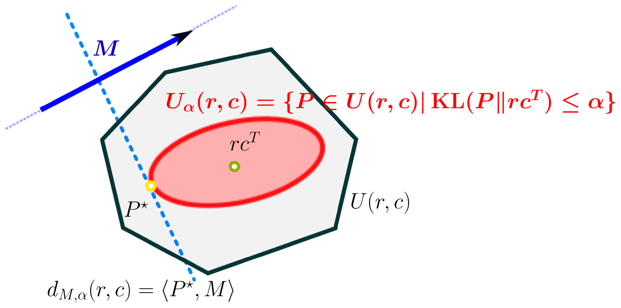
$ U_\alpha(r,c)\operatorname{\overset{\operatorname{def}}{=}} {P\in U(r,c),|, \mathbf{KL}(P|rc^T)\leq \alpha } = {P\in U(r,c),|, h(P)\geq h(r)+h(c)-\alpha} $

These definitions are indeed equivalent, since one can easily check that

$ \mathbf{KL}(P|rc^T)= h(r)+h(c)-h(P), $

a quantity which is also the mutual information $I(X|Y)$ of two random variables $(X,Y)$ should they follow the joint probability $P$ ([19], §2). Hence, all tables $P$ whose Kullback-Leibler divergence to the table $rc^T$ is constrained to lie below a certain threshold can be interpreted as the set of tables $P$ in $U(r,c)$ which have sufficient entropy with respect to $h(r)$ and $h(c)$, or joint probabilities which display a small enough mutual information.

As a classic result of linear optimization, the optimum of classical optimal transportation distances is achieved on vertices of $U(r,c)$, that is $d\times d$ matrices with only up to $2d-1$ non-zero elements ([21], §8.1.3). Such plans can be interpreted as quasi-deterministic joint probabilities, since if $p_{ij}>0$, then very few values $p_{ij'}$ will have a non-zero probability. By mitigating the transportation cost objective with an entropic constraint, which is equivalent to following the max-entropy principle ([22, 23]) and thus for a given level of the cost look for the most smooth joint probability, we argue that we can provide a more robust notion of distance between histograms. Indeed, for a given pair $(r,c)$, finding plausible transportation plans with low cost (where plausibility is measured by entropy) is more informative than finding extreme plans that are extremely unlikely to appear in nature.

We note that the idea of regularizing the transportation problem was also considered recently by [24]. In their work, [24] also argue that an optimal matching may not be sufficiently regular in vision applications (color transfer), and that these undesirable properties can be handled through an adequate relaxation and penalization (through graph-based norms) of the transportation problem. While [24] penalize the transportation problem to obtain a more regular transportation plan, we believe that an entropic regularization yields here a better distance. An illustration of this idea is provided in Figure 1. For reasons that will become clear in Section 4, we call such distances Sinkhorn distances.

########## {caption="Definition 1: Sinkhorn Distances"}

$\displaystyle d_{M,\alpha}(r,c)\operatorname{\overset{\operatorname{def}}{=}}\min_{P\in U_\alpha(r,c)}{\langle P , M,\rangle}$

3.2 Metric Properties

When $\alpha$ is large enough, the Sinkhorn distance coincides with the classic optimal transportation distance. When $\alpha=0$, the Sinkhorn distance has a closed form and becomes a negative definite kernel if one assumes that $M$ is itself a negative definite distance, that is a Euclidean distance matrix.

########## {caption="Property 2"}

For $\alpha$ large enough, the Sinkhorn distance $d_{M,\alpha}$ is the transportation distance $d_{M}$.

Proof: Since for any $P\in U(r,c), h(P)$ is lower bounded by $\tfrac{1}{2}(h(r)+h(c))$, we have that for $t$ large enough $U_{t}(r,c)= U(r,c)$ and thus both quantities coincide.

########## {caption="Property: Independence Kernel"}

When $\alpha=0$ and $M$ is a Euclidean Distance Matrix[^1], the Sinkhorn distance has the explicit form $d_{M,0}=r^T M c$. $d_{M,0}$ is a negative definite kernel, i.e. $e^{-t r^TMc}$ is a positive definite kernel $\forall t>0$. We call this kernel the independence kernel.

[^1]: $\exists n, \exists \varphi_1,\cdots,\varphi_d\in \mathbb{R}^n$ such that $m_{ij}=\lVert{\varphi_i - \varphi_j}\rVert_2^2$ ([25], §5). Recall that, in that case, $M.^t=[m_{ij}^t]$, $0<t<1$ is also a Euclidean distance matrix ([26], p.78, §3.2.10)

The proof is provided in the appendix. Beyond these two extreme cases, the main theorem of this section states that Sinkhorn distances are symmetric and satisfy triangle inequalities for all possible values of $\alpha$. Since for $\alpha$ small enough $d_{M,\alpha}(r,r)>0$ for any $r$ such that $h(r)>0$, Sinkhorn distances cannot satisfy the coincidence axiom[^2]. However, multiplying $d_{M,\alpha}$ by $\mathbf 1_{r\ne c}$ suffices to recover the coincidence property if needed.

[^2]: satisfied if $d(x,y)=0\Leftrightarrow x=y$ holds for all $x,y$

########## {caption="Theorem 3"}

For all $\alpha\geq 0$ and $M\in \mathcal{M}$, $d_{M,\alpha}$ is symmetric and satisfies all triangle inequalities. The function $(r,c)\mapsto \mathbf 1_{r\ne c} d_{M,\alpha}(r,c)$ satisfies all three distance axioms.

The gluing lemma ([27], Lemma 7.6) plays a crucial role to prove that optimal transportation distances are indeed distances. The version we use below is slightly different since it incorporates the entropic constraint.

########## {caption="Lemma 4: Gluing Lemma With Entropic Constraint"}

Let $\alpha\geq 0$ and $x,y,z$ be three elements of $\Sigma_d$. Let $P\in U_\alpha(x,y)$ and $Q\in U_\alpha(y,z)$ be two joint probabilities in the transportation polytopes of $(x,y)$ and $(y,z)$ with sufficient entropy. Let $S$ be the $d\times d$ matrix whose $(i,k)

The proof is provided in the appendix. We can prove the triangle inequality for $d_{M,\alpha}$ by using the same proof strategy than that used for classical transportation distances.

Proof of Theorem 3. The symmetry of $d_{M,\alpha}$ is a direct result of $M

$ \begin{aligned} d_{M,\alpha}(x,z)&=\min_{P\in U_\alpha(x,z)}{\langle X , M,\rangle} \leq {\langle S , M,\rangle} = \sum_{ik} m_{ik}\sum_{j} \frac{p_{ij}q_{jk}}{y_j} \ & \leq \sum_{ijk} \left(m_{ij}+m_{jk}\right) \frac{p_{ij}q_{jk}}{y_j} = \sum_{ijk} m_{ij} \frac{p_{ij}q_{jk}}{y_j} +m_{jk} \frac{p_{ij}q_{jk}}{y_j} \ & =\sum_{ij} m_{ij}p_{ij} \sum_k \frac{q_{jk}}{y_j} + \sum_{jk} m_{jk} q_{jk} \sum_i \frac{p_{ij}}{y_j}\ &= \sum_{ij} m_{ij}p_{ij} + \sum_{jk} m_{jk} q_{jk} = d_{M,\alpha}(x,y)+d_{M,\alpha}(y,z).,\square\end{aligned} $

4. Computing Sinkhorn Distances with the Sinkhorn-Knopp Algorithm

Section Summary: The section explains how the Sinkhorn distance can be relaxed by introducing a Lagrange multiplier on the entropy constraint, yielding a dual formulation called the dual-Sinkhorn divergence that is far cheaper to compute than exact optimal transport. This relaxed problem has a unique solution of a simple factored form, which the classical Sinkhorn-Knopp fixed-point iteration can recover efficiently from the cost matrix and the two marginals; a short vectorized algorithm implements the procedure and extends immediately to many histograms at once. The authors therefore adopt this approximation for the rest of the paper, noting that its entropy can be driven toward the target value by adjusting the multiplier if needed.

Recall that the Sinkhorn distance (Definition 1) is defined through a hard constraint on the entropy of $h(P)$ relative to $h(r)$ and $h(c)$. In what follows, we consider the same program with a Lagrange multiplier for the entropy constraint,

$ \boxed{d_{M}^{\lambda}(r,c) \operatorname{\overset{\operatorname{def}}{=}} {\langle P^\lambda , M,\rangle},,\text{ where } P^\lambda= \mathop{argmin}_{P\in U(r,c)} {\langle P , M,\rangle} - \frac{1}{\lambda} h(P).} $

By duality theory we have that for every pair $(r,c)$, to each $\alpha$ corresponds an $\lambda\in[0,\infty]$ such that $d_{M,\alpha(r,c)}=d_{M}^{\lambda}(r,c)$. We call $d_{M}^\lambda$ the dual-Sinkhorn divergence and show that it can be computed at a much cheaper cost than the classical optimal transportation problem for reasonable values of $\lambda$.

4.1 Computing $d_{M}^\lambda$

When $\lambda>0$, the solution $P^\lambda$ is unique by strict convexity of minus the entropy. In fact, $P^\lambda$ is necessarily of the form $u_i e^{-\lambda m_{ij}} v_j$, where $u$ and $v$ are two non-negative vectors uniquely defined up to a multiplicative factor.

Input `M`, $\lambda$, `r`, `c`.
I=(r>0); r=r(I); M=M(I,:); K=exp(- $\lambda$*M)
Set `x`=`ones(length(r),size(c,2))/length(r)`;
while `x` changes do
  `x=diag(1./r)*K*(c.*(1./(K'*(1./x))))`
end while
`u=1./x; v=c.*(1./(K'*u))`
$d_{M}^\lambda$ (`r`,`c`)=`sum(u.*((K.*M)*v))`

This well known fact in transportation theory ([12]) can be indeed checked by forming the Lagrangian $\mathcal{L}(P,\alpha,\beta)$ of the objective of Equation 2 using $\alpha,\beta\geq \mathbf{0}_d$ for each of the two equality constraints in $U(r,c)$. For these two cost vectors $\alpha,\beta$,

$ \mathcal{L}(P,\alpha,\beta)=\sum_{ij} \frac{1}{\lambda}p_{ij}\log p_{ij}+ p_{ij}m_{ij} + \alpha^T(P \mathbf 1_d-r) + \beta^T(P^T \mathbf 1_d-c) $

We obtain then, for any couple $(i,j)$, that if $\frac{\partial \mathcal{L}}{\partial p_{ij}^\lambda}=0$, then

$ p_{ij}^\lambda= e^{-\frac{1}{2}-\lambda \alpha_i} e^{-\lambda m_{ij}}e^{-\frac{1}{2}-\lambda \beta_j}, $

and thus recover the form provided above. $P^\lambda$ is thus, by [13]'s theorem [13], the only matrix with row-sum $r$ and column-sum $c$ of the form

$ \exists u,v>\mathbf{0}_d : P^\lambda = \mathop{diag}(u) e^{-\lambda M} \mathop{diag}(v). $

Given $e^{-\lambda M}$ and marginals $r$ and $c$, it is thus sufficient to run enough iterations of [13]'s algorithm to converge to a solution $P^\lambda$ of that problem. We provide a one line implementation in Algorithm 1. The case where some coordinates of $r$ or $c$ are null can be easily handled by selecting those elements of $r$ that are strictly positive to obtain the desired table, as shown in the first line of Algorithm 1. Note that Algorithm 1 is vectorized: it can be used as such to compute the distance between $r$ and a family of histograms $C=[c_1,\cdots,c_N]$ by replacing $c$ with $C$. These $O(d^2N)$ linear algebra operations can be very quickly executed by using a GPGPU.

4.2 Computing $d_{M,\alpha}$ through $d_{M}^\lambda$

With a naive approach, $d_{M,\alpha}$ can be obtained by computing $d_{M}^\lambda$ iteratively until the entropy of the solution $P^\lambda$ has reached an adequate value $h(r)+h(c)-\alpha$. Since the entropy of $P^\lambda$ decreases monotonically when $\lambda$ increases, this search can be carried out by simple bisection, starting with a small $\lambda$ which is iteratively increased. In what follows, we only consider the dual-Sinkhorn divergence $d_{M}^\lambda$ since it is cheaper to compute and displays good performances in itself. We believe that more clever approaches can be applied to calculate exactly $d_{M,\alpha}$, and we leave this for future work. In the rest of this paper we will now refer to $d_{M}^\lambda$ as the Sinkhorn distance, despite the fact that it is not provably a distance.

5. Experimental Results

Section Summary: On the MNIST handwritten digit dataset, experiments converted each image into a normalized histogram over a 20-by-20 pixel grid and compared Sinkhorn distances against several standard alternatives for SVM-based classification. Across multiple training-set sizes and repeated cross-validation folds, the Sinkhorn approach produced lower average error rates than the Hellinger, chi-squared, total-variation, Euclidean, independence, and even classical earth-mover’s distances. Additional tests confirmed that the Sinkhorn values remain within roughly 10 percent of exact optimal-transport distances while running orders of magnitude faster on both CPU and GPU hardware.

5.1 MNIST Digits

We test the performance of Sinkhorn distances on the MNIST digits^3 dataset, on which the ground metric has a natural interpretation in terms of pixel distances. Each digit is provided as a vector of intensities on a $20\times 20$ pixel grid. We convert each image into a histogram by normalizing each pixel intensity by the total sum of all intensities . We consider a subset of $N$ points in the training set of the database, where $N$ ranges within ${3,5,12,17,25}\times 10^3$ datapoints.

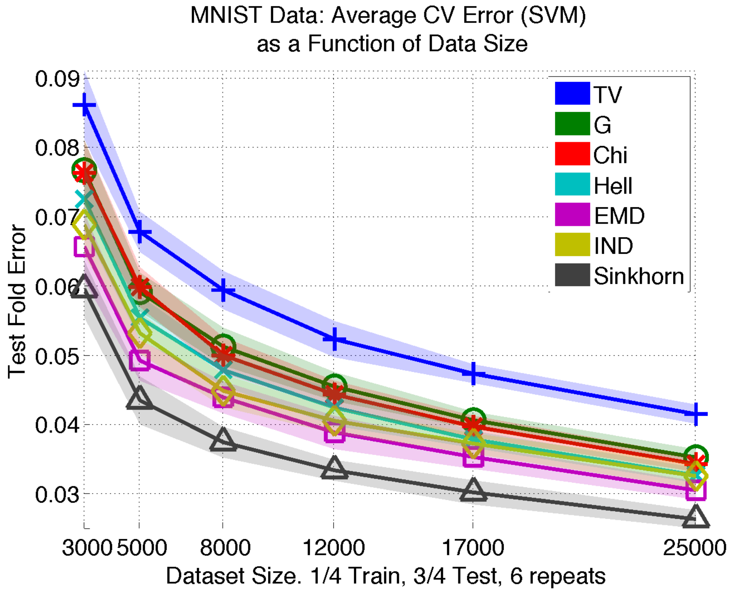
5.1.1 Experimental setting

For each subset of size $N$, we provide mean and standard deviation of classification error using a 4 fold (3 test, 1 train) cross validation scheme repeated 6 times, resulting in 24 different experiments. We study the performance of different distances with the following parameter selection scheme: for each distance $d$, we consider the kernel $e^{-d/t}$, where $t>0$ is chosen by cross validation individually for each training fold within the set ${1,q_{10}(d),q_{20}(d),q_{50}(d)}$, where $q_s$ is the $s%$ quantile of a subset of distances observed in the training fold. We regularize non-positive definite kernel matrices resulting from this computation by adding a sufficiently large diagonal term. SVM's were run with libsvm (one-vs-one) for multiclass classification, the regularization constant $C$ being selected by 2 folds/2 repeats cross-validation on the training fold in the set $10^{-2:2:4}$

5.1.2 Distances

The Hellinger, $\chi_2$, Total Variation and squared Euclidean (Gaussian kernel) distances are used as such. We set the ground metric $M$ to be the Euclidean distance between the $20\times 20$ points in the grid, resulting in a $400\times 400$ distance matrix. We also tried to use Mahalanobis distances on this example with a positive definite matrix equal to exp(-tM.\^{}2), t>0, as well as its inverse, with varying values of $t$ but none of the results proved competitive. For the Independence kernel, since any Euclidean distance matrix is valid, we consider $[m_{ij}^a]$ where $a\in{0.01,0.1,1}$ and choose $a$ by cross-validation on the training set. Smaller values of $a$ seem to be preferable. We select the entropic penalty $\lambda$ of Sinkhorn distances so that the matrix $e^{-\lambda M}$ is relatively diagonally dominant and the resulting transportation not too far from the classic optimal transportation. We select $\lambda$ for each training fold by internal cross-validation within ${5,7,9,11}\times 1/q_{50}(M)$ where $q_{50}(M)$ is the median distance between pixels on the grid. We set the number of fixed-point iterations to an arbitrary number of 20 iterations. In most (though not all) folds, the value $\lambda=9$ comes up as the best setting. The Sinkhorn distance beats by a safe margin all other distances, including the EMD.

5.2 Does the Sinkhorn Distance Converge to the EMD?

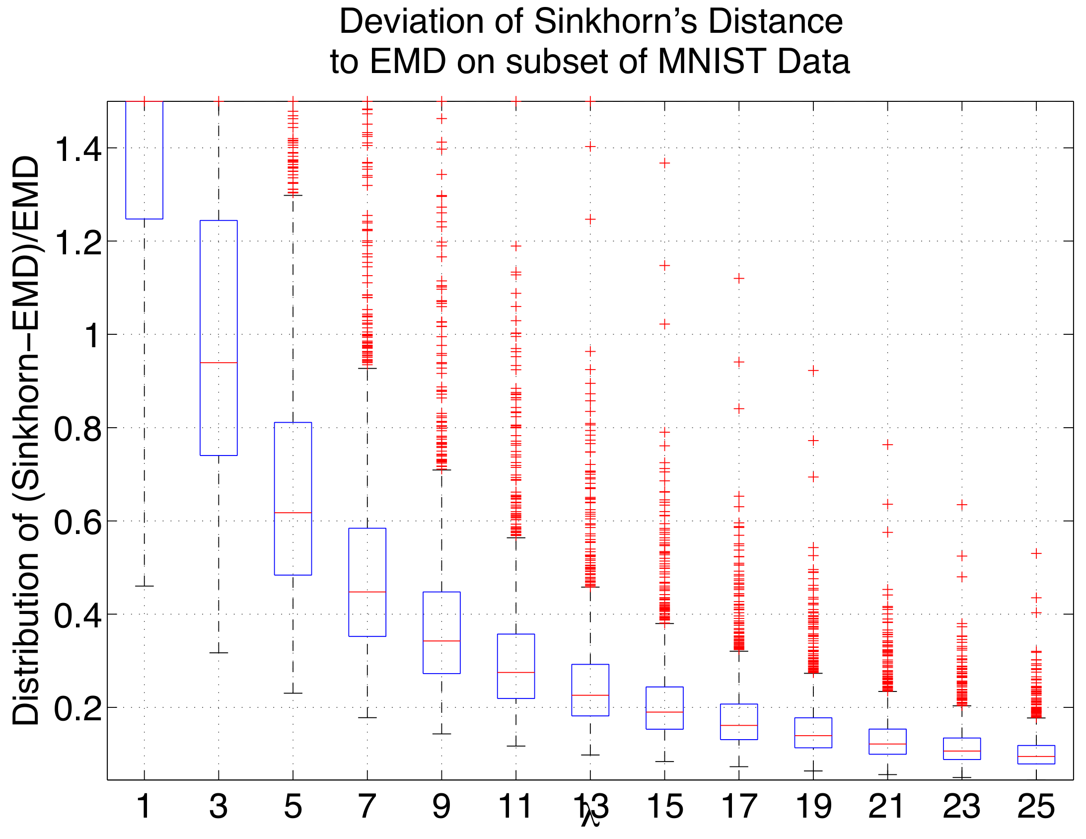
We study in this section the convergence of Sinkhorn distances towards classical optimal transportation distances as $\lambda$ gets bigger. Because of the additional penalty that appears in Equation 2 program, $d_{M}^\lambda(r,c)$ is necessarily larger than $d_M(r,c)$, and we expect this gap to decrease as $\lambda$ increases. Figure 3 illustrates this by plotting the boxplot of distributions of $(d_{M}^\lambda(r,c)-d_M(r,c))/d_M(r,c)$ over $40^2$ pairs of distinct points taken in the MNIST database. As can be observed, even with large values of $\lambda$, Sinkhorn distances hover above the values of EMD distances by about $10%$. For practical values of $\lambda$ such as $\lambda=9$ selected above we do not expect the Sinkhorn distance to be numerically close to the EMD, nor believe it to be a desirable property.

5.3 Several Orders of Magnitude Faster

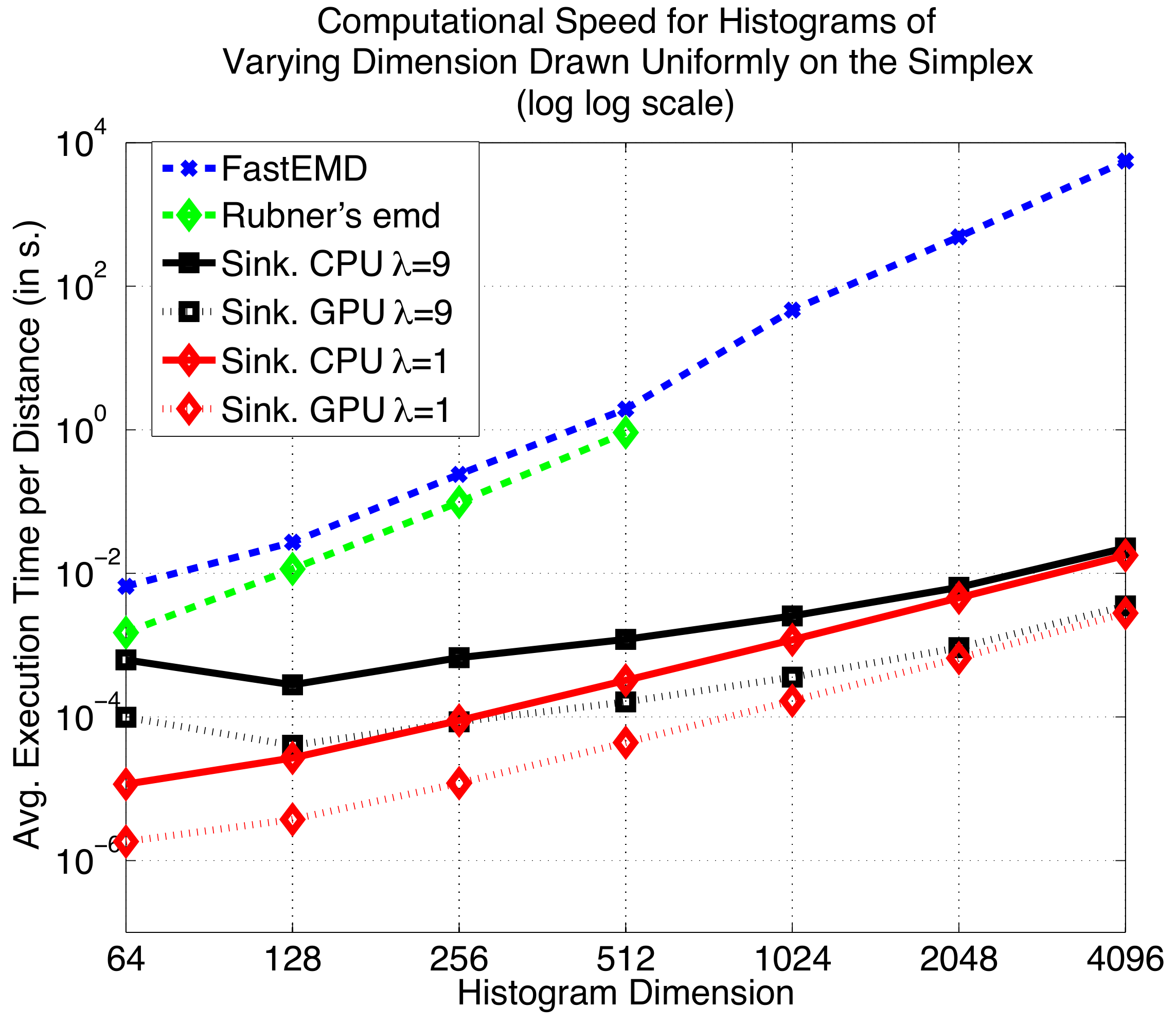
We measure in this section the computational speed of classic optimal transportation distances vs. that of Sinkhorn distances using [2]'s 2 and [11]'s [11][^5] publicly available implementations. We generate points uniformly in the $d$-simplex ([28]) and generate random distance matrices $M$ by selecting $d$ points distributed with a spherical Gaussian in dimension $d/10$ to obtain enough variability in the distance matrix. $M$ is then divided by the median of its values, $\texttt{M=M/median(M(:))}$. Sinkhorn distances are implemented in matlab code (see Algorithm 1) while emd_mex, emd_hat_gd_metric are mex/C files. The emd distances and Sinkhorn CPU are run on a matlab session with a single working core (2.66 Ghz Xeon). Sinkhorn GPU is run on an NVidia Quadro K5000 card. Following the experimental findings of Section 5.1, we consider two parameters for $\lambda$, $\lambda=1$ and $\lambda=9$. $\lambda=1$ results in a relatively dense matrix $K=e^{-\lambda M}$, with results comparable to that of the Independence kernel, while $\lambda=9$ results in a matrix $K=e^{-\lambda M}$ with mostly negligible values and therefore a matrix with low entropy that is closer to the optimal transportation solution. [2]'s implementation cannot be run for histograms larger than $d=512$. For large dimensions and on the same CPU, Sinkhorn distances are more than 100.000 faster than EMD solvers given a threshold of $0.01$. Using a GPU results in a speed-up of a supplementary order of magnitude.

[^5]: http://www.cs.huji.ac.il/~ofirpele/FastEMD/code/, we use emd_hat_gd_metric in these experiments

5.4 Empirical Complexity

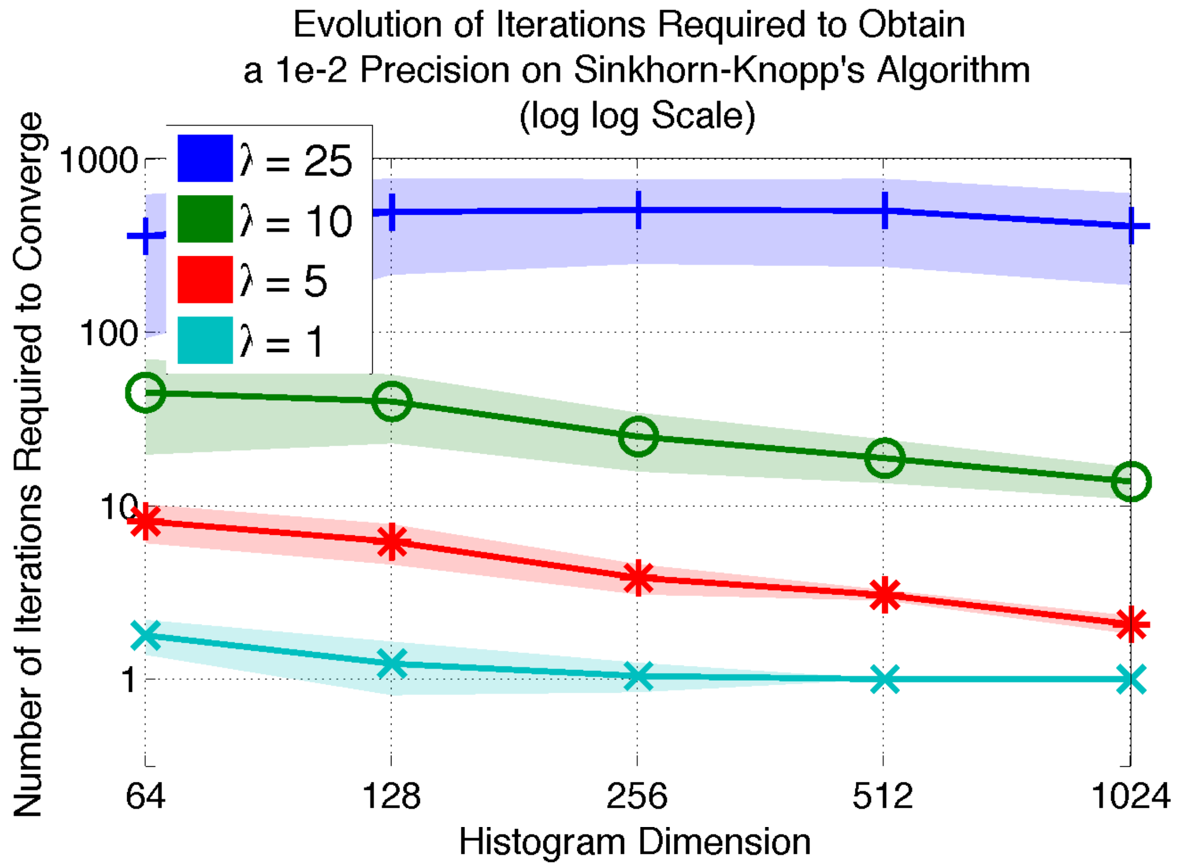
To provide an accurate picture of the actual number of steps required to guarantee the algorithm's convergence, we replicate the experiments of Section 5.3 but focus now on the number of iterations of the loop described in Algorithm 1. We use a tolerance of $0.01$ on the norm of the difference of two successive iterations of $x\in \mathbb{R}^d$. As can be seen in Figure 5, the number of iterations required so that $\lVert x-x'\rVert_2\leq 0.01$ increases as $e^{-\lambda M}$ becomes diagonally dominant. From a practical perspective, and because keeping track of the change of $x$ at each iteration can be costly on parallel platforms, we recommend setting a fixed number of iterations that only depends on the value of $\lambda$. With that modification, and when computing the distance of a point $r$ to a family of points $C$, we obtain speedups by using GPGPU's which are even larger than those displayed in Figure 4.

6. Conclusion

Section Summary: Adding a simple penalty term based on entropy to the classic optimal transport problem makes the computations much faster, no matter what underlying distance measure is used. This leads to Sinkhorn distances that perform at least as well as standard methods like the Earth Mover's Distance, and sometimes better, when applied to machine learning tasks. The single adjustable parameter in this approach does not appear to create any meaningful trade-off between speed and accuracy.

We have shown that regularizing the optimal transportation problem with an intuitive entropic penalty opens the door for new research directions and potential applications at the intersection of optimal transportation theory and machine learning. This regularization guarantees speed-ups that are effective whatever the structure of the ground metric $M$. Based on preliminary evidence, it seems that Sinkhorn distances do not perform worse than the EMD, and may in fact perform better in applications. Sinkhorn distances are parameterized by a regularization weight $\lambda$ which should be tuned having both computational and performance objectives in mind, but we have not observed a need to establish a trade-off between both. Indeed, reasonably small values of $\lambda$ seem to perform better than large ones.

7. Appendix: Proofs

Section Summary: The appendix presents two technical proofs supporting earlier claims in the paper. The first demonstrates that a kernel formed from a negative definite matrix yields a negative definite function on pairs of probability distributions, by rewriting the expression using vector embeddings and known properties of such kernels, along with a note on efficient computation. The second constructs an auxiliary joint distribution that forms a valid transport plan between two marginals and applies the data processing inequality for Markov chains to establish a bound on joint entropy.

Proof of Property 2: The set $U_1(r,c)$ contains all joint probabilities $P$ for which $h(P)=h(r)+h(c)$. In that case ([19], Theorem 2.6.6) applies and $U_1(r,c)$ can only be equal to the singleton ${rc^T}$. If $M$ is negative definite, there exists vectors $(\varphi_1,\cdots,\varphi_d)$ in some Euclidean space $\mathbb{R}^n$ such that $m_{ij}=\lVert{\varphi_i-\varphi_j}\rVert_2^2$ through ([26], §3.3.2). We thus have that

$ \begin{aligned}r^TM c&= \sum_{ij}r_i c_j \lVert{\varphi_i-\varphi_j}\rVert^2= (\sum_{i}r_i \lVert{\varphi_i}\rVert^2 + \sum_{i} c_i \lVert{\varphi_i}\rVert^2) - 2\sum_{ij} {\langle r_i\varphi_i , c_j\varphi_j,\rangle}\&= r^Tu + c^Tu - 2 r^TK c\end{aligned} $

where $u_i=\lVert{\phi_i}\rVert^2$ and $K_{ij}={\langle \varphi_i , \varphi_j,\rangle}$. We used the fact that $\sum r_i=\sum c_i=1$ to go from the first to the second equality. $r^TMc$ is thus a n.d. kernel because it is the sum of two n.d. kernels: the first term $(r^Tu+c^Tu)$ is the sum of the same function evaluated separately on $r$ and $c$, and thus a negative definite kernel ([26], §3.2.10); the latter term $-2r^TKu$ is negative definite as minus a positive definite kernel ([26], Definition §3.1.1).

Remark. The proof above suggests a faster way to compute the Independence kernel. Given a matrix $M$, one can indeed pre-compute the vector of norms $u$ as well as a Cholesky factor $L$ of $K$ above to preprocess a dataset of histograms by premultiplying each observations $r_i$ by $L$ and only store $Lr_i$ as well as precomputing its diagonal term $r_i^Tu$. Note that the independence kernel is positive definite on histograms with the same 1-norm, but is no longer positive definite for arbitrary vectors.

Proof of Lemma 4: Let $T$ be the a probability distribution on ${1,\cdots,d}^d$ whose coefficients are defined as

$ t_{ijk}\operatorname{\overset{\operatorname{def}}{=}} \frac{p_{ij}q_{jk}}{y_j}, $

for all indices $j$ such that $y_j>0$. For indices $j$ such that $y_j=0$, all values $t_{ijk}$ are set to $0$.

Let $S \operatorname{\overset{\operatorname{def}}{=}} [ \sum_{j} t_{ijk}]_{ik}$. $S$ is a transportation matrix between $x$ and $z$. Indeed,

$ \begin{aligned} \sum_{i} \sum_{j} s_{ijk}&= \sum_{j} \sum_{i}\frac{p_{ij}q_{jk}}{y_j}= \sum_{j} \frac{q_{jk}}{y_j} \sum_{i} p_{ij} =\sum_{j} \frac{q_{jk}}{y_j} y_j=\sum_j q_{jk}=z_k \text{ (column sums) }\ \sum_{k} \sum_{j} s_{ijk}&= \sum_{j} \sum_{k}\frac{p_{ij}q_{jk}}{y_j}= \sum_{j} \frac{p_{ij}}{y_j} \sum_{k}q_{jk} =\sum_{j} \frac{p_{ij}}{y_j} y_j=\sum_j p_{ij}=x_i \text{ (row sums) } \end{aligned} $

We now prove that $h(S)\geq h(x)+h(z)-\alpha$. Let $(X,Y,Z)$ be three random variables jointly distributed as $T$. Since by definition of $T$ in Equation 4

$ p(X,Y,Z)=p(X,Y)p(Y,Z)/p(Y)= p(X)p(Y|X)p(Z|Y), $

the triplet $(X,Y,Z)$ is a Markov chain $X\rightarrow Y \rightarrow Z$ ([19], Equation 2.118) and thus, by virtue of the data processing inequality ([19], Theorem 2.8.1), the following inequality between mutual informations applies:

$ I(X;Y)\geq I(X;Z),\text{ namely } \quad h(X,Z)-h(X)+h(Z)\geq h(X,Y) -h(X)+h(Y)\geq -\alpha. $

References

Section Summary: This section compiles 28 academic citations that underpin research on optimal transport and the earth mover's distance. The listed works span foundational texts on transportation problems and probability metrics, along with papers on fast computational algorithms, approximations for image and histogram comparison, and connections to matrix scaling, network flows, and information theory. Together they trace the development of both theoretical results and practical methods across mathematics, computer vision, and statistics.

[1] Villani, C. (2009). Optimal transport: old and new, volume 338. Springer Verlag.

[2] Rubner, Y., Guibas, L., and Tomasi, C. (1997). The earth mover’s distance, multi-dimensional scaling, and color-based image retrieval. In Proceedings of the ARPA Image Understanding Workshop, pages 661–668.

[3] Levina, E. and Bickel, P. (2001). The earth mover's distance is the mallows distance: some insights from statistics. In Proceedings of the Eighth IEEE International Conference on Computer Vision, volume 2, pages 251–256. IEEE.

[4] Indyk, P. and Thaper, N. (2003). Fast image retrieval via embeddings. In 3rd International Workshop on Statistical and Computational Theories of Vision (at ICCV).

[5] Naor, A. and Schechtman, G. (2007). Planar earthmover is not in l$_{1}$. SIAM J. Comput., 37(3):804–826.

[6] Andoni, A., Ba, K. D., Indyk, P., and Woodruff, D. (2009). Efficient sketches for earth-mover distance, with applications. In Foundations of Computer Science (FOCS) 2009., pages 324 –330.

[7] Grauman, K. and Darrell, T. (2004). Fast contour matching using approximate earth mover's distance. In IEEE Conf. Vision and Patt. Recog., pages 220–227.

[8] Ling, H. and Okada, K. (2007). An efficient earth mover's distance algorithm for robust histogram comparison. IEEE transactions on Patt. An. and Mach. Intell., pages 840–853.

[9] Gudmundsson, J., Klein, O., Knauer, C., and Smid, M. (2007). Small manhattan networks and algorithmic applications for the earth mover’s distance. In Proceedings of the 23rd European Workshop on Computational Geometry, pages 174–177.

[10] Shirdhonkar, S. and Jacobs, D. (2008). Approximate earth mover’s distance in linear time. In CVPR 2008, pages 1–8. IEEE.

[11] Pele, O. and Werman, M. (2009). Fast and robust earth mover's distances. In ICCV'09.

[12] Erlander, S. and Stewart, N. (1990). The gravity model in transportation analysis: theory and extensions. Vsp.

[13] Sinkhorn, R. and Knopp, P. (1967). Concerning nonnegative matrices and doubly stochastic matrices. Pacific J. Math, 21(2):343–348.

[14] Knight, P. A. (2008). The sinkhorn-knopp algorithm: convergence and applications. SIAM Journal on Matrix Analysis and Applications, 30(1):261–275.

[15] Ahuja, R., Magnanti, T., and Orlin, J. (1993). Network Flows: Theory, Algorithms and Applications. Prentice Hall.

[16] Orlin, J. B. (1993). A faster strongly polynomial minimum cost flow algorithm. Operations research, 41(2):338–350.

[17] Avis, D. (1980). On the extreme rays of the metric cone. Canadian Journal of Mathematics, 32(1):126–144.

[18] Brickell, J., Dhillon, I., Sra, S., and Tropp, J. (2008). The metric nearness problem. SIAM J. Matrix Anal. Appl, 30(1):375–396.

[19] Cover, T. and Thomas, J. (1991). Elements of Information Theory. Wiley & Sons.

[20] Good, I. (1963). Maximum entropy for hypothesis formulation, especially for multidimensional contingency tables. The Annals of Mathematical Statistics, pages 911–934.

[21] Brualdi, R. A. (2006). Combinatorial matrix classes, volume 108. Cambridge University Press.

[22] Jaynes, E. T. (1957). Information theory and statistical mechanics. Phys. Rev., 106:620–630.

[23] Dudík, M. and Schapire, R. E. (2006). Maximum entropy distribution estimation with generalized regularization. In Learning Theory, pages 123–138. Springer.

[24] Ferradans, S., Papadakis, N., Rabin, J., Peyré, G., Aujol, J.-F., et al. (2013). Regularized discrete optimal transport. In International Conference on Scale Space and Variational Methods in Computer Vision, pages 1–12.

[25] Dattorro, J. (2005). Convex optimization & Euclidean distance geometry. Meboo Publishing USA.

[26] Berg, C., Christensen, J., and Ressel, P. (1984). Harmonic Analysis on Semigroups. Number 100 in Graduate Texts in Mathematics. Springer Verlag.

[27] Villani, C. (2003). Topics in Optimal Transportation, volume 58. AMS Graduate Studies in Mathematics.

[28] Smith, N. A. and Tromble, R. W. (2004). Sampling uniformly from the unit simplex. Johns Hopkins University, Tech. Rep, 10:15–20.