Three-dimensional alpha shapes

Herbert EdelsbrunnerErnst Mücke

article1994TOG2,165 citations

Introduces three-dimensional alpha shapes alongside a quadratic-time construction algorithm, providing a mathematically rigorous framework to extract multiscale geometric structures and boundaries from discrete 3D point sets.

Listen

Scientific computing and 3D visualization applications frequently generate large point clouds representing physical phenomena, ranging from molecular structures to astronomical distributions. However, computer science historically lacked a mathematically rigorous, computable definition of the intuitive geometric concept of "shape" in three dimensions, forcing practitioners to rely on subjective heuristics or rigid convex hulls. The article resolves this limitation by introducing the formal concept of three-dimensional alpha shapes, a parameterized family of geometric shapes derived from a point set that spans the spectrum from fine local detail to a global bounding outline.

The article establishes a solid theoretical foundation and algorithmic framework for constructing 3D alpha shapes, while validating practical implementation feasibility through experimental benchmarks. To achieve this, the authors utilize Delaunay triangulations and Voronoi diagrams to represent the underlying spatial relationships of a point set. By defining an "alpha-ball" that carves out empty space, geometric simplexes—vertices, edges, triangles, and tetrahedra—are classified as interior, regular, or singular across intervals of alpha values. The authors implemented a three-step software pipeline consisting of an incremental flipping algorithm for Delaunay triangulation, an alpha-interval generator, and an interactive rendering tool, testing the system across twenty diverse empirical and synthetic datasets containing up to 15,000 points.

The evaluation reveals four primary findings. First, a point set of size n produces at most 2n^2 - 5n distinct alpha shapes, enabling the entire continuous spectrum of shapes to be compactly captured as a discrete family. Second, while the worst-case construction time is quadratic, the practical execution time scales much closer to n(log n)^2 across typical datasets. Third, exact long-integer arithmetic is essential for robust geometric computing; runtime profiling shows that approximately 75% of total CPU time is spent on long-integer calculations to resolve geometric tests. Fourth, symbolic perturbation eliminates topological failures caused by degenerate data, such as coplanar or cospherical points, guaranteeing algorithm correctness without requiring costly manual geometric case analysis.

These findings have direct operational implications for engineering, computational biology, and physics. By providing a unified mathematical framework, alpha shapes enable automated mesh generation, cavity and tunnel identification in protein folding studies, and objective quantification of galaxy clustering without arbitrary heuristics. Because exact integer arithmetic dominates processing overhead, high-throughput applications will benefit substantially from optimized mathematical libraries or specialized hardware acceleration rather than relying on standard floating-point approximations that risk topological corruption.

Organizations handling geometric 3D data should consider adopting alpha shapes as a standard modeling primitive, particularly when structural connectivity and multi-scale feature detection are required. Immediate next steps for technical teams include evaluating output-sensitive triangulation algorithms and randomized flipping methods to optimize construction speeds for large volumetric grid data. Furthermore, developers should pursue the implementation of weighted alpha shapes for multi-sized atomic models and dynamic update algorithms to avoid recomputing full triangulations during iterative spatial simulations.

The findings are supported by strong mathematical proofs and consistent experimental benchmarks across diverse datasets. However, a key limitation of the current implementation is its degraded performance on regular grid structures, which trigger higher computational overhead than non-uniform point distributions. Stakeholders should maintain high confidence in the mathematical rigor and robustness of the tool, while noting that extreme dataset sizes or dynamic point movements may require upcoming algorithmic enhancements before deploying in real-time processing pipelines.

University of Illinois Urbana-Champaign parallel computing scientific computing Three-dimensional alpha shapes Delaunay triangulations regular triangulations

arXiv: math/9410208

No sufficiently relevant recommendations were found.

Cover for Three-dimensional alpha shapes

Abstract

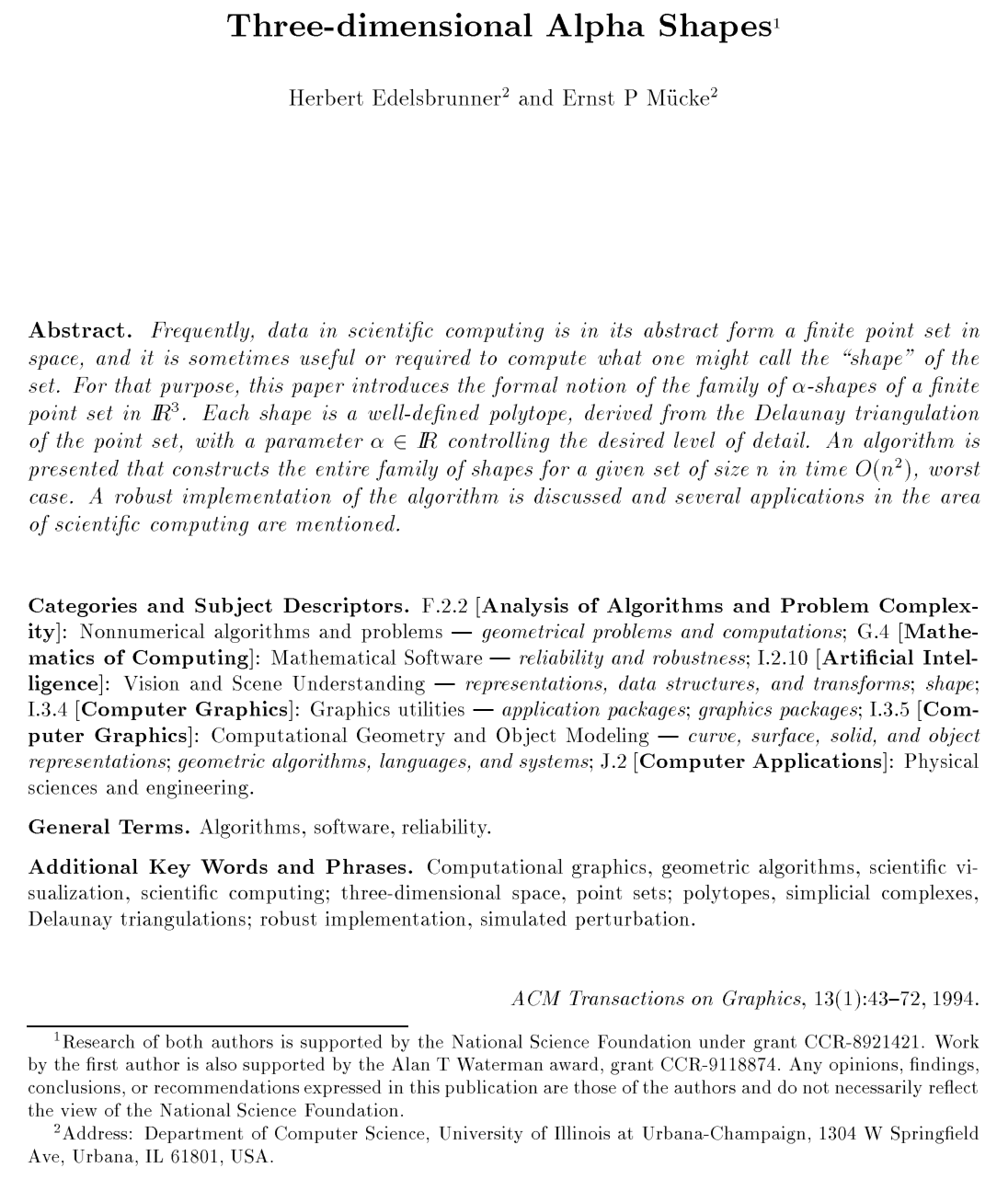
Frequently, data in scientific computing is in its abstract form a finite point set in space, and it is sometimes useful or required to compute what one might call the ``shape'' of the set. For that purpose, this paper introduces the formal notion of the family of $\alpha$ -shapes of a finite point set in $\Real^3$ . Each shape is a well-defined polytope, derived from the Delaunay triangulation of the point set, with a parameter $\alpha \in \Real$ controlling the desired level of detail. An algorithm is presented that constructs the entire family of shapes for a given set of size $n$ in time $O(n^2)$ , worst case. A robust implementation of the algorithm is discussed and several applications in the area of scientific computing are mentioned.

Topics

parallel computing scientific computing

Keywords

Three-dimensional alpha shapes Delaunay triangulations regular triangulations Voronoi diagrams convex polytopes computational geometry scientific visualization

1 Introduction
2 Alpha Shapes in Space
3 Related Geometric Concepts
3.1 Alpha Hulls and Alpha Diagrams
3.2 Delaunay Triangulations and Voronoi Diagrams
3.3 Alpha Complexes
3.4 Extensions
4 Combinatorial Analysis
5 Algorithms
5.1 Three-dimensional Delaunay Triangulations
5.2 Intervals and Face Classification
5.3 Geometric Primitives
6 Implementation
6.1 Data Structures
6.2 Simulated Perturbation
6.3 Performance
7 Applications and Further Illustrations
8 Summary and Open Problems
Available Software
Acknowledgements
References

Knowls

Knowl 1 — Three-Dimensional Alpha Complex and Alpha Shape
definition
Let $S \subset \mathbb{R}^3$ be a finite point set in general position, and let $\alpha \in \mathbb{R}$ satisfy $0 \le \alpha \le \infty$ . An open ball of radius $\alpha$ is called an $\alpha$ -ball (with a $0$ -ball defined as a single point and an $\infty$ -ball as an open half-space). An $\alpha$ -ball $b$ is empty if $b \cap S = \emptyset$ .

Let $\mathcal{D}$ denote the Delaunay triangulation of $S$ . For any subset $T \subseteq S$ of size $|T| = k+1$ with $0 \le k \le 3$ , $\sigma_T = \operatorname{conv}(T)$ is a $k$ -simplex of $\mathcal{D}$ . The smallest sphere containing all points of $T$ is denoted $\partial b_T$ , with radius $\rho_T$ and open interior $b_T$ . For $k=3$ , $\partial b_T$ is the circumsphere; for $k=2$ , the circumcircle of $\sigma_T$ is a great circle of $\partial b_T$ ; for $k=1$ , the two points in $T$ are antipodal on $\partial b_T$ .

For $1 \le k \le 3$ , define $G_{k,\alpha}$ as the set of $k$ -simplices $\sigma_T \in \mathcal{D}$ for which $b_T$ is empty and $\rho_T < \alpha$ . Define $G_{0,\alpha} = S$ for all $\alpha$ .

The $\alpha$ -complex $\mathcal{C}_\alpha$ of $S$ is the simplicial complex whose $k$ -simplices either belong to $G_{k,\alpha}$ or bound a $(k+1)$ -simplex of $\mathcal{C}_\alpha$ . For $0 \le \alpha_1 \le \alpha_2$ , $\mathcal{C}_{\alpha_1}$ is a subcomplex of $\mathcal{C}_{\alpha_2}$ .

The $\alpha$ -shape of $S$ , denoted $S_\alpha$ , is the underlying space (the point set union of all simplices) of the $\alpha$ -complex:

$S_\alpha = |\mathcal{C}_\alpha| = \bigcup_{\sigma \in \mathcal{C}_\alpha} \sigma$

Equivalently, the boundary $\partial S_\alpha$ consists of $\alpha$ -exposed simplices, where a $k$ -simplex $\sigma_T$ ( $0 \le k \le 2$ ) is $\alpha$ -exposed if there exists an empty $\alpha$ -ball $b$ with $T = \partial b \cap S$ .

Knowl 2 — Classification and Interval Decomposition of Simplices in Alpha Complexes

theoretical result

For any simplex $\sigma_T \in \mathcal{D}$ , the range of parameter values $\alpha$ for which $\sigma_T \in \mathcal{C}_\alpha$ forms a single continuous interval. Within this interval, each simplex $\sigma_T \in \mathcal{C}_\alpha$ is categorized into one of three mutually exclusive states:

interior: $\sigma_T \not\in \partial S_\alpha$ ,
regular: $\sigma_T \in \partial S_\alpha$ and $\sigma_T$ bounds some higher-dimensional simplex in $\mathcal{C}_\alpha$ ,
singular: $\sigma_T \in \partial S_\alpha$ and $\sigma_T$ does not bound any higher-dimensional simplex in $\mathcal{C}_\alpha$ .

A simplex $\sigma_T \in \mathcal{D}$ is called attached if $|T| \in \{2, 3\}$ and its smallest open circumsphere $b_T$ contains at least one point of $S$ ( $b_T \cap S \neq \emptyset$ ); otherwise, it is unattached.

Let $\operatorname{up}_1(\sigma_T) = \{ \sigma_{T'} \in \mathcal{D} \mid T \subset T', |T'| = |T| + 1 \}$ denote the set of simplices of one dimension higher incident to $\sigma_T$ . The transition thresholds $\underline{\mu}_T$ (singular to regular) and $\overline{\mu}_T$ (regular to interior) are defined recursively:

If $\sigma_T$ is a tetrahedron ( $|T|=4$ ): $\underline{\mu}_T = \overline{\mu}_T = \rho_T$ .
If $|T| \le 3$ :

$\underline{\mu}_T = \min \left( \{ \rho_{T'} \mid \sigma_{T'} \in \operatorname{up}_1(\sigma_T), \sigma_{T'} \text{ unattached} \} \cup \{ \underline{\mu}_{T'} \mid \sigma_{T'} \in \operatorname{up}_1(\sigma_T), \sigma_{T'} \text{ attached} \} \right)$

$\overline{\mu}_T = \max \{ \overline{\mu}_{T'} \mid \sigma_{T'} \in \operatorname{up}_1(\sigma_T) \}$

The intervals of $\alpha$ for which $\sigma_T$ is singular, regular, or interior depend on whether $\sigma_T$ is on the convex hull boundary $\partial \operatorname{conv}(S)$ :

Simplex type	Position	Singular	Regular	Interior
tetrahedron				$(\rho_T, \infty]$
edge / triangle	$\notin \partial\operatorname{conv}(S)$ , unattached	$(\rho_T, \underline{\mu}_T)$	$(\underline{\mu}_T, \overline{\mu}_T)$	$(\overline{\mu}_T, \infty]$
edge / triangle	$\notin \partial\operatorname{conv}(S)$ , attached		$(\underline{\mu}_T, \overline{\mu}_T)$	$(\overline{\mu}_T, \infty]$
edge / triangle	$\in \partial\operatorname{conv}(S)$ , unattached	$(\rho_T, \underline{\mu}_T)$	$(\underline{\mu}_T, \infty]$
edge / triangle	$\in \partial\operatorname{conv}(S)$ , attached		$(\underline{\mu}_T, \infty]$
vertex	$\notin \partial\operatorname{conv}(S)$	$[0, \underline{\mu}_T)$	$(\underline{\mu}_T, \overline{\mu}_T)$	$(\overline{\mu}_T, \infty]$
vertex	$\in \partial\operatorname{conv}(S)$	$[0, \underline{\mu}_T)$	$(\underline{\mu}_T, \infty]$

Knowl 3 — Upper Bound on the Number of Distinct Alpha Shapes
theoretical result
For a finite point set $S \subset \mathbb{R}^3$ of size $n = |S| \ge 5$ in general position, the family of all $\alpha$ -shapes as $\alpha$ ranges over $[0, \infty]$ contains at most $2n^2 - 5n$ distinct shapes.

This bound is established by mapping the point set $S$ to $\mathbb{R}^4$ via the lifting map:

$p = (\pi_1, \pi_2, \pi_3) \mapsto p^U = \left(\pi_1, \pi_2, \pi_3, \sum_{i=1}^3 \pi_i^2\right)$

The Delaunay triangulation $\mathcal{D}$ corresponds to the projection of the lower boundary of the convex hull of the lifted points $S^U = \{p^U \mid p \in S\} \subset \mathbb{R}^4$ . By the Upper Bound Theorem for convex polytopes in $\mathbb{R}^4$ , the maximum numbers of $k$ -simplices in $\mathcal{D}$ (sets $F_k$ ) are:

$|F_0| = n, \quad |F_1| \le \frac{1}{2}(n^2 - n), \quad |F_2| \le n^2 - 3n, \quad |F_3| \le \frac{1}{2}(n^2 - 3n - 2)$

Because two shapes $S_{\alpha_1} \neq S_{\alpha_2}$ differ only when the interval $[\alpha_1, \alpha_2]$ contains the circumradius $\rho_T$ of an unattached simplex in $\mathcal{D}$ , the number of distinct shapes is at most one plus the total number of simplices of dimension 1, 2, and 3 in $\mathcal{D}$ :

$1 + |F_1| + |F_2| + |F_3| \le 1 + \frac{1}{2}(n^2 - n) + (n^2 - 3n) + \frac{1}{2}(n^2 - 3n - 2) = 2n^2 - 5n$
Knowl 4 — Algorithm for Computing Simplex Alpha Intervals and Alpha Spectrum
algorithm
Given the Delaunay triangulation $\mathcal{D}$ of a point set $S \subset \mathbb{R}^3$ where each simplex is flagged as belonging to $\partial\operatorname{conv}(S)$ or not, this algorithm computes the state intervals for all simplices and constructs the sorted $\alpha$ -spectrum.
Input: Delaunay triangulation $\mathcal{D}$ of point set $S$ , with convex hull boundary flags
Output: Classification intervals $(\rho_T, \underline{\mu}_T, \overline{\mu}_T)$ for every $\sigma_T \in \mathcal{D}$ , and sorted $\alpha$ -spectrum
for each edge and triangle $\sigma_T \in \mathcal{D}$ do
    Classify $\sigma_T$ as attached if any incident simplex in $\operatorname{up}_1(\sigma_T)$ contains a vertex inside $b_T$ ; otherwise unattached
end for
for each tetrahedron $\sigma_T \in \mathcal{D}$ do
    Compute $\rho_T$
    Set $\underline{\mu}_T = \rho_T$ and $\overline{\mu}_T = \rho_T$
end for
for each triangle $\sigma_T \in \mathcal{D}$ in decreasing order of dimension do
    Compute $\rho_T$ if unattached
     $\underline{\mu}_T = \min(\{ \rho_{T'} \mid \sigma_{T'} \in \operatorname{up}_1(\sigma_T), \text{unattached}\} \cup \{ \underline{\mu}_{T'} \mid \sigma_{T'} \in \operatorname{up}_1(\sigma_T), \text{attached}\})$
     $\overline{\mu}_T = \max(\{ \overline{\mu}_{T'} \mid \sigma_{T'} \in \operatorname{up}_1(\sigma_T)\})$
end for
for each edge $\sigma_T \in \mathcal{D}$ do
    Compute $\rho_T$ if unattached
    Compute $\underline{\mu}_T$ and $\overline{\mu}_T$ from $\operatorname{up}_1(\sigma_T)$
end for
for each vertex $\sigma_T \in \mathcal{D}$ do
    Compute $\underline{\mu}_T$ and $\overline{\mu}_T$ from $\operatorname{up}_1(\sigma_T)$
end for
Collect all $\rho_T$ values of unattached simplices ( $1 \le k \le 3$ ), append $0$ and $\infty$ , remove duplicates, and sort to produce the $\alpha$ -spectrum
Classifying all simplices and computing $\underline{\mu}_T, \overline{\mu}_T$ takes $O(m)$ time, where $m = |\mathcal{D}|$ is the number of simplices in $\mathcal{D}$ . Sorting the non-duplicate $\alpha$ -thresholds takes $O(m \log m)$ time.
Knowl 5 — Exact Determinant Formulas for Geometric Primitives and Circumsphere Radii
equation
Let points $p_i \in \mathbb{R}^3$ be defined by coordinate vectors $(\pi_{i,1}, \pi_{i,2}, \pi_{i,3})$ , with $\pi_{i,0} = 1$ and $\pi_{i,4} = \sum_{j=1}^3 \pi_{i,j}^2$ . Minors are denoted by:

$M_{j_1, j_2, \dots, j_k}^{i_1, i_2, \dots, i_k} = \det \begin{pmatrix} \pi_{i_1, j_1} & \pi_{i_1, j_2} & \dots & \pi_{i_1, j_k} \\ \pi_{i_2, j_1} & \pi_{i_2, j_2} & \dots & \pi_{i_2, j_k} \\ \vdots & \vdots & \ddots & \vdots \\ \pi_{i_k, j_1} & \pi_{i_k, j_2} & \dots & \pi_{i_k, j_k} \end{pmatrix}$

Plane Orientation Test: For $T = (p_i, p_j, p_k)$ , point $p_u$ lies on the positive side of plane $h_T$ if and only if:

$M_{1,2,3,0}^{i,j,k,u} > 0$

Sphere Test: For $T = \{p_i, p_j, p_k, p_u\}$ , point $p_v$ lies inside the circumsphere $\partial b_T$ if and only if:

$M_{1,2,3,0}^{i,j,k,u} \cdot M_{1,2,3,4,0}^{i,j,k,u,v} > 0$

Squared Radius $\rho_T^2$ of Smallest Circumsphere:
- Edge $T = \{p_i, p_j\}$ :
$\rho_T^2 = \frac{(M_{1,0}^{i,j})^2 + (M_{2,0}^{i,j})^2 + (M_{3,0}^{i,j})^2}{4}$
- Triangle $T = \{p_i, p_j, p_k\}$ :
$\rho_T^2 = \frac{\left(\sum_{\ell=1}^3 (M_{\ell,0}^{i,j})^2\right) \cdot \left(\sum_{\ell=1}^3 (M_{\ell,0}^{j,k})^2\right) \cdot \left(\sum_{\ell=1}^3 (M_{\ell,0}^{k,i})^2\right)}{4 \left( (M_{2,3,0}^{i,j,k})^2 + (M_{1,3,0}^{i,j,k})^2 + (M_{1,2,0}^{i,j,k})^2 \right)}$
- Tetrahedron $T = \{p_i, p_j, p_k, p_u\}$ :
$\rho_T^2 = \frac{(M_{2,3,4,0}^{i,j,k,u})^2 + (M_{1,3,4,0}^{i,j,k,u})^2 + (M_{1,2,4,0}^{i,j,k,u})^2 + 4 M_{1,2,3,0}^{i,j,k,u} M_{1,2,3,4}^{i,j,k,u}}{4 (M_{1,2,3,0}^{i,j,k,u})^2}$
Knowl 6 — Formulas for Testing Attached and Unattached Simplices
equation
An edge or triangle $\sigma_T \in \mathcal{D}$ is attached if an incident higher-dimensional simplex $\sigma_R \in \operatorname{up}_1(\sigma_T)$ contains its opposite vertex inside the open smallest circumsphere $b_T$ of $\sigma_T$ .

Edge Attachment Test: For edge $T = \{p_i, p_j\}$ and adjacent vertex $p_k$ (where $R = \{p_i, p_j, p_k\}$ ), $p_k \in b_T$ if and only if:

$\sum_{\ell=1}^3 (M_{\ell,0}^{i,j})^2 - \sum_{\ell=1}^3 (M_{\ell,0}^{i,k} + M_{\ell,0}^{j,k})^2 > 0$

where $M_{\ell,0}^{a,b} = \pi_{a,\ell} - \pi_{b,\ell}$ .

Triangle Attachment Test: For triangle $T = \{p_i, p_j, p_k\}$ and adjacent vertex $p_u$ in tetrahedron $R = \{p_i, p_j, p_k, p_u\}$ , $p_u \in b_T$ if and only if the circumcenter $c$ of $\partial b_R$ and $p_u$ lie on opposite sides of the plane spanned by $T$ , given by:

$M_{2,3,4,0}^{i,j,k,u} M_{2,3,0}^{i,j,k} + M_{1,3,4,0}^{i,j,k,u} M_{1,3,0}^{i,j,k} + M_{1,2,4,0}^{i,j,k,u} M_{1,2,0}^{i,j,k} - 2 M_{1,2,3,0}^{i,j,k,u} M_{1,2,3}^{i,j,k} > 0$

where $\pi_{a,4} = \sum_{\ell=1}^3 \pi_{a,\ell}^2$ and minors $M$ are determinants of the corresponding coordinate submatrices.
Knowl 7 — Simulation of Simplicity (SoS) for Geometric Predicates
model/method
To handle degeneracies (such as coplanar or cospherical points) without explicit case analysis, the Simulation of Simplicity (SoS) technique replaces the coordinate $\pi_{i,j}$ of point $p_i \in S$ ( $1 \le j \le 3$ ) with a symbolically perturbed coordinate:

$\pi_{i,j}(\varepsilon) = \pi_{i,j} + \varepsilon(i, j), \quad \text{where } \varepsilon(i, j) = \varepsilon^{\delta^{4i-j}}$

for a sufficiently large constant $\delta$ and an infinitesimal parameter $\varepsilon > 0$ .

Geometric predicates are evaluated by expanding the corresponding matrix determinants into polynomials in $\varepsilon$ :

$P(\varepsilon) = C_0 + C_1 \varepsilon^{e_1} + C_2 \varepsilon^{e_2} + \dots$

where terms are sorted by strictly increasing powers of $\varepsilon$ . The sign of the predicate is determined by the sign of the lowest-degree coefficient $C_t$ that does not vanish (the evaluation has depth $t$ ). Exact long-integer arithmetic is used to evaluate the polynomial coefficients $C_t$ , ensuring consistency and non-degeneracy while adding zero numerical error.
Knowl 8 — Incremental-Flip Construction of Three-Dimensional Delaunay Triangulations
algorithm
Three-dimensional Delaunay triangulations are constructed incrementally by point insertion and local bistellar flips (Joe's algorithm).
Input: Point set $S = \{p_1, p_2, \dots, p_n\} \subset \mathbb{R}^3$
Output: Delaunay triangulation $\mathcal{D}$ of $S$
Sort $S$ along a fixed direction, relabeling points as $p_1, p_2, \dots, p_n$
Initialize $\mathcal{D}$ as the single tetrahedron $\operatorname{conv}(\{p_1, p_2, p_3, p_4\})$
for $i = 5$ to $n$ do
    Add $p_i$ by connecting it to all vertices, edges, and triangles of $\mathcal{D}$ visible from $p_i$
    while there exists an interior triangle $\sigma_T$ shared by tetrahedra $\sigma_{T'}$ and $\sigma_{T''}$ that is not locally Delaunay do
        if $\sigma_{T'} \cup \sigma_{T''}$ is convex then
            Execute triangle-to-edge flip (replace 2 tetrahedra sharing $\sigma_T$ with 3 tetrahedra sharing the edge connecting the opposite vertices)
        else if there exists a third tetrahedron $\sigma_{T'''}$ forming a non-convex configuration of 3 tetrahedra sharing an edge then
            Execute edge-to-triangle flip (replace 3 tetrahedra sharing an edge with 2 tetrahedra sharing a triangle)
        end if
    end while
end for
A triangle $\sigma_T$ shared by tetrahedra $\sigma_{T \cup \{p_u\}}$ and $\sigma_{T \cup \{p_v\}}$ is locally Delaunay if $p_v$ lies outside the circumsphere $\partial b_{T \cup \{p_u\}}$ . The worst-case time and storage complexity is $O(n^2)$ .
Knowl 9 — Triangle-Edge Data Structure for 3D Simplicial Complexes
model/method
The triangle-edge structure is a specialized, compact representation of 3D simplicial cell complexes derived from the general edge-facet structure.

The atomic unit is the triangle-edge pair $a = \langle \sigma, i \rangle$ with $0 \le i \le 5$ , representing triangle $\sigma$ associated with one of its six directed edges. The structure maintains two topological cycles for every simplex:
- Edge rings: Two cyclic orderings of length 3 traversing the directed edges of $\sigma$ (one clockwise, one counterclockwise).
- Triangle rings: Two cyclic orderings traversing the triangles incident to a directed edge in opposite rotational directions.
Because all edge rings have a fixed length of 3, explicit pointers for edge ring traversal are omitted by merging the six triangle-edge pairs of the two opposite edge rings into a single record. Each record requires 30 bytes per triangle when using 2-byte vertex indices and 4-byte triangle-edge identifiers (or 36 bytes when using 4-byte vertex indices).
Knowl 10 — Computational Overhead of Exact Arithmetic in Alpha Shape Construction
empirical result
Experimental profiling of the incremental-flip Delaunay triangulation and $\alpha$ -interval generation algorithms shows that practical performance scales roughly as $O(n (\log n)^2)$ for typical point distributions, significantly better than the $O(n^2)$ theoretical worst-case.

Exact arithmetic accounts for the majority of the computational workload:
- Approximately 75% of overall CPU time is spent on exact long-integer arithmetic evaluating determinant minors for SoS predicates and circumsphere radii.
- Long-integer multiplication routines alone consume more than half of the exact arithmetic computation time.
- Highly degenerate input sets (e.g., points on regular grids or parallel slices) trigger higher evaluation depths in SoS (maximum depths up to 39 terms) and substantially increase the number of flips and determinant calculations compared to non-degenerate inputs of equal size.

Coverage note — Omitted brief discussions of non-3D / weighted extensions (such as negative alpha shapes via furthest-point Delaunay, weighted alpha shapes via regular triangulations, and higher-dimensional generalizations) as well as UI details of the Alvis visualization software, as they are not the core analytical contributions of this paper.

References

1.J D Boissonnat. Geometric structures for three-dimensional shape representation. ACM Transactions on Graphics, 3(4):266–286, 1984.
2.E Brisson. Representing geometric structures in d dimensions: Topology and order. Discrete and Computational Geometry, 9(4):387–426, 1993.
3.A Brønsted. An Introduction to Convex Polytopes. Graduate Texts in Mathematics. Springer-Verlag, New York, 1983.
4.R Y Cen, A Jameson, F Liu, and J P Ostriker. The universe in a box: Thermal effects in a standard cold dark matter scenario. Astrophysical Journal (Letters), 362:L41, 1990.
5.T H Cormen, C E Leiserson, and R L Rivest. Introduction to Algorithms. MIT Press, Cambridge, Massachusetts, 1990.
6.B Delaunay. Sur la sphère vide. Izvestia Akademii Nauk SSSR, Otdelenie Matematicheskii i Estestvennyka Nauk, 7:793–800, 1934.
7.D P Dobkin and M J Laszlo. Primitives for the manipulation of three-dimensional subdivisions. Algorithmica, 4(1):3–32, 1989.
8.R A Drebin, L Carpenter, and P Hanrahan. Volume rendering. Computer Graphics, 22(4):65–74, 1988. ACM Siggraph '88. Conference Proceedings.
9.R A Dwyer. Higher-dimensional Voronoi diagrams in linear expected time. Discrete and Computational Geometry, 6(4):343–367, 1991.
10.M D Dyksterhouse. An alpha-shape view of our universe. Master's thesis, Department of Computer Science, University of Illinois at Urbana-Champaign, Urbana, Illinois, 1992.
11.H Edelsbrunner. Algorithms in Combinatorial Geometry. Springer-Verlag, Berlin, 1987.
12.H Edelsbrunner. Geometric algorithms. In P Gruber and J Wills, editors, Handbook of Convex Geometry, pages 699–735. North-Holland, Amsterdam, 1992.
13.H Edelsbrunner. Weighted alpha shapes. Technical Report UIUCDCS-R-92-1760, Department of Computer Science, University of Illinois at Urbana-Champaign, Urbana, Illinois, 1992.
14.H Edelsbrunner, D G Kirkpatrick, and R Seidel. On the shape of a set of points in the plane. IEEE Transactions on Information Theory, IT-29(4):551–559, 1983.
15.H Edelsbrunner and E P Mücke. Simulation of Simplicity: A technique to cope with degenerate cases in geometric algorithms. ACM Transactions on Graphics, 9(1):66–104, 1990.
16.H Edelsbrunner and N R Shah. Incremental topological flipping works for regular triangulations. In Proceedings of the Eighth Annual Symposium on Computational Geometry, pages 43–52, 1992.
17.J Fairfield. Contoured shape generation: Forms that people see in dot patterns. In Proceedings of the IEEE Conference on Cybernetics and Society, pages 60–64, 1979.
18.J Fairfield. Segmenting dot patterns by Voronoi diagram concavity. IEEE Transactions on Pattern Analysis and Machine Intelligence, 5(1):104–110, 1983.
19.M J Geller and J P Huchra. Mapping the universe. Science, 246:897–903, 1989.
20.C Ghélis and J Yon. Protein Folding. Academic Press, 1982.
21.P J Giblin. Graphs, Surfaces, and Homology. Second edition. Chapman and Hall, London, 1981.
22.L J Guibas and J Stolfi. Primitives for manipulation of general subdivisions and the computation of Voronoi diagrams. ACM Transactions on Graphics, 4(2):74–123, 1985.
23.R A Jarvis. Computing the shape hull of points in the plane. In Proceedings of the IEEE Computing Society Conference on Pattern Recognition and Image Processing, pages 231–241, 1977.
24.B Joe. Three-dimensional triangulations from local transformations. SIAM Journal on Scientific and Statistical Computing, 10(4):718–741, 1989.
25.B Joe. Construction of three-dimensional Delaunay triangulations using local transformations. Computer Aided Geometric Design, 8(2):123–142, 1991.
26.D G Kirkpatrick and J D Radke. A framework for computational morphology. In G T Toussaint, editor, Computational Geometry, pages 234–244. Elsevier North Holland, New York, 1985.
27.C L Lawson. Software for $C^1$ surface interpolation. In J R Rice, editor, Mathematical Software III, pages 161–194. Academic Press, New York, 1977.
28.C Lee. Regular triangulations of convex polytopes. In P Gritzmann and B Sturmfels, editors, Applied Geometry and Discrete Mathematics: The Victor Klee Festschrift, pages 443–456. American Mathematical Society, Providence, RI, 1991.
29.W E Lorensen and H E Cline. Marching cubes: A high resolution 3D surface construction algorithm. Computer Graphics, 21(4):163–169, 1987. ACM Siggraph '87. Conference Proceedings.
30.J Matoušek and O Schwarzkopf. Linear optimization queries. In Proceedings of the Eighth Annual Symposium on Computational Geometry, pages 16–25, 1992.
31.D W Matula and R R Sokal. Properties of Gabriel graphs relevant to geographic variation research and the clustering of points in the plane. Geographical Analysis, 12(3):205–222, 1980.
32.P McMullen and G C Shepard. Convex Polytopes and the Upper Bound Conjecture. Cambridge Unversity Press, London, 1971.
33.W W Moss. Some new analytic and graphic approaches to numerical taxonomy, with an example from the Dermanyssidae (Acari). Systematic Zoology, 16:177–207, 1967.
34.E P Mücke. Shapes and Implementations in Three-Dimensional Geometry. PhD thesis, Department of Computer Science, University of Illinois at Urbana-Champaign, Ubana, Illinois, 1993. Also as Technical Report UIUCDCS-R-93-1836.
35.F P Preparata and M I Shamos. Computational Geometry — An Introduction. Springer-Verlag, New York, 1985.
36.F M Richards. The protein folding problem. Scientific American, 264(1):54–63, 1991.
37.R Seidel. Constructing higher-dimensional convex hulls in logarithmic cost per face. In Proceedings of the 18th Annual ACM Symposium on Theory of Computing, pages 484–507, 1986.
38.R Seidel. Exact upper bounds for the number of faces in d-dimensional Voronoi diagrams. In P Gritzmann and B Sturmfels, editors, Applied Geometry and Discrete Mathematics: The Victor Klee Festschrift, pages 517–530. American Mathematical Society, Providence, RI, 1991.
39.G T Toussaint. The relative neighborhood graph of a finite planar set. Pattern Recognition, 12(4):261–268, 1980.
40.R C Veltkamp. Closed Object Boundaries from Scattered Points. PhD thesis, Erasmus Universiteit, Rotterdam, 1992.
41.G Voronoi. Nouvelles applications des paramètres continus à la théorie des formes quadratiques. Premier Mémoire: Sur quelques propriétés des formes quadratiques positives parfaites. Journal für die Reine und Angewandte Mathematik, 133:97–178, 1907.
42.G Voronoi. Nouvelles applications des paramètres continus à la théorie des formes quadratiques. Deuxième Mémoire: Recherches sur les parallélloèdres primitifs. Journal für die Reine und Angewandte Mathematik, 134:198–287, 1908.

Citation

MLA

Edelsbrunner, H., and E. Mücke. “Three-dimensional Alpha Shapes”. arXiv, 1994, http://arxiv.org/abs/math/9410208v1.

APA

Edelsbrunner, H., & Mücke, E. (1994). Three-dimensional alpha shapes. arXiv. http://arxiv.org/abs/math/9410208v1

Chicago

Edelsbrunner, H., and E. Mücke. 1994. “Three-dimensional Alpha Shapes”. arXiv. http://arxiv.org/abs/math/9410208v1.

Harvard

Edelsbrunner, H. and Mücke, E. (1994) “Three-dimensional alpha shapes”, arXiv [Preprint]. Available at: http://arxiv.org/abs/math/9410208v1.

Vancouver

1. Edelsbrunner H, Mücke E (1994) Three-dimensional alpha shapes. arXiv

BibTeX

@article{edelsbrunner1994three,
  title = {Three-dimensional alpha shapes},
  author = {Edelsbrunner, Herbert and Mücke, Ernst},
  year = {1994},
  journal = {arXiv},
  url = {http://arxiv.org/abs/math/9410208v1},
  eprint = {math/9410208}
}

Metadata:arXiv

Access the Paper

This paper is available from its original source. Click below to access the PDF.

Open PDF

Three-dimensional alpha shapes

Abstract

Topics

Keywords

Table of Contents

Knowls

Knowl 1 — Three-Dimensional Alpha Complex and Alpha Shape

Knowl 2 — Classification and Interval Decomposition of Simplices in Alpha Complexes

Knowl 3 — Upper Bound on the Number of Distinct Alpha Shapes

Knowl 4 — Algorithm for Computing Simplex Alpha Intervals and Alpha Spectrum

Knowl 5 — Exact Determinant Formulas for Geometric Primitives and Circumsphere Radii

Knowl 6 — Formulas for Testing Attached and Unattached Simplices

Knowl 7 — Simulation of Simplicity (SoS) for Geometric Predicates

Knowl 8 — Incremental-Flip Construction of Three-Dimensional Delaunay Triangulations

Knowl 9 — Triangle-Edge Data Structure for 3D Simplicial Complexes

Knowl 10 — Computational Overhead of Exact Arithmetic in Alpha Shape Construction

References

Citation

BibTeX

Access the Paper