Data Validation For Machine Learning

Eric Breck $^{1}$ Neoklis Polyzotis $^{1}$ Sudip Roy $^{1}$ Steven Euijong Whang $^{2}$ Martin Zinkevich $^{1}$

$^{1}$ Google Research $^{2}$ KAIST. Work done while at Google Research. Correspondence to: Neoklis Polyzotis [email protected].

ABSTRACT

Machine learning is a powerful tool for gleaning knowledge from massive amounts of data. While a great deal of machine learning research has focused on improving the accuracy and efficiency of training and inference algorithms, there is less attention in the equally important problem of monitoring the quality of data fed to machine learning. The importance of this problem is hard to dispute: errors in the input data can nullify any benefits on speed and accuracy for training and inference. This argument points to a data-centric approach to machine learning that treats training and serving data as an important production asset, on par with the algorithm and infrastructure used for learning.

In this paper, we tackle this problem and present a data validation system that is designed to detect anomalies specifically in data fed into machine learning pipelines. This system is deployed in production as an integral part of TFX (Baylor et al., 2017) – an end-to-end machine learning platform at Google. It is used by hundreds of product teams use it to continuously monitor and validate several petabytes of production data per day. We faced several challenges in developing our system, most notably around the ability of ML pipelines to soldier on in the face of unexpected patterns, schema-free data, or training/serving skew. We discuss these challenges, the techniques we used to address them, and the various design choices that we made in implementing the system. Finally, we present evidence from the system’s deployment in production that illustrate the tangible benefits of data validation in the context of ML: early detection of errors, model-quality wins from using better data, savings in engineering hours to debug problems, and a shift towards data-centric workflows in model development.

Executive Summary: Machine learning models power critical applications like recommendations, health diagnostics, and autonomous vehicles, but they rely on vast amounts of data that often contain errors. These errors, stemming from bugs in data generation code or mismatches between training and real-world serving data, can degrade model performance, amplify through feedback loops, and cause costly production failures. With ML pipelines handling petabytes of data daily, undetected issues lead to wasted engineering effort, unreliable predictions, and lost opportunities for innovation. Addressing data quality is essential now, as organizations scale ML from experiments to production, where reliability directly impacts business outcomes.

This paper evaluates and demonstrates a data validation system designed to monitor and catch errors in input data for machine learning pipelines. The goal is to ensure data integrity at every stage, from ingestion to serving, treating data as a core asset alongside algorithms and infrastructure.

The authors developed their system within Google's TensorFlow Extended (TFX), an end-to-end ML platform, drawing from database principles but adapting them for ML's unique needs, such as schema-free formats and evolving data streams. They focused on three validation types: checking individual data batches for anomalies using precomputed statistics and a user-defined schema that specifies expected feature types, ranges, and presence; comparing batches over time or between training and serving to detect shifts, like distribution changes or feature mismatches; and testing training code with synthetic data generated from the schema to uncover hidden assumptions, such as invalid mathematical operations. The system processes full batches (not samples) for accuracy, infers initial schemas from historical data, and suggests updates as data evolves. It was deployed across hundreds of product teams, analyzing trillions of examples—several petabytes daily—over real production pipelines spanning months.

The system revealed several key insights. First, schemas evolve actively: in over 700 pipelines, most underwent 1-5 manual updates, confirming data's natural changes without excessive volatility. Second, common anomalies included new or missing features (affecting 6-10% of pipelines daily) and out-of-domain values (like unexpected categories in 6% of cases), with over 50-80% of alerts leading to fixes, such as code patches or schema revisions. Third, model unit tests ran over 80,000 times monthly, failing in 6% of cases to expose code-data mismatches. Case studies showed tangible gains: one recommender fixed serving-training gaps, boosting app installs by 2%; another team resolved parsing errors in two days, achieving model parity during infrastructure migration; and some teams used the system standalone for monitoring without full retraining.

These findings underscore that proactive data validation prevents error propagation, saving engineering hours on debugging and enabling higher model quality. For instance, early alerts avoid training flawed models, reducing risks in high-stakes applications like recommendations or self-driving tech. Unlike expectations of static data, the results highlight ML's dynamic nature, where skew between training and serving—often from code path differences—can subtly erode performance. This shifts workflows toward data-centric practices, where schemas document features and facilitate team collaboration, ultimately cutting costs and improving compliance with production standards.

Leaders should integrate similar validation into ML platforms organization-wide, starting with schema inference for quick setup and prioritizing alerts for high-impact anomalies like feature drifts. For pipelines already in use, run standalone validation to baseline data health. Trade-offs include initial schema curation effort versus long-term gains; automated tools minimize this, but human review ensures relevance. Next steps involve piloting in new domains, like structured data formats, and expanding to automated root-cause analysis. Further work could refine schema inference to reduce overfit risks.

While robust in production, the system has limitations: it covers most but not all error types, relying on heuristics for schema generation that may miss nuanced domain knowledge, and alerts depend on human operators who might overlook them under load. Confidence is high for detected anomalies based on deployment scale and fixes rates, but caution is advised for rare, slice-specific issues or unmodeled data evolutions—additional monitoring of model outputs could complement it.

1 INTRODUCTION

Section Summary: Machine learning is increasingly applied in fields like healthcare and self-driving cars, where reliable platforms help deploy complex data pipelines, but the quality of input data is crucial to avoid errors that degrade models and worsen over time through feedback loops. The paper emphasizes treating data as a core element in these pipelines, needing ongoing monitoring and validation tools, while borrowing from database techniques but adapting them to ML's unique challenges. An example from Google shows how a subtle code bug can introduce persistent errors in data slices, making detection difficult due to decoupled data sources and raw formats, and highlighting the need for precise alerts to help engineers quickly fix underlying code issues.

Machine Learning (ML) is widely used to glean knowledge from massive amounts of data. The applications are ever-increasing and range from machine perception and text understanding to health care, genomics, and self-driving cars. Given the critical nature of some of these applications, and the role that ML plays in their operation, we are also observing the emergence of ML platforms (Baylor et al., 2017; Chandra, 2014) that enable engineering teams to reliably deploy ML pipelines in production.

In this paper we focus on the problem of validating the input data fed to ML pipelines. The importance of this problem is hard to overstate, especially for production pipelines. Irrespective of the ML algorithms used, data errors can adversely affect the quality of the generated model. Furthermore, it is often the case that the predictions from the generated models are logged and used to generate more data for training. Such feedback loops have the potential to amplify even “small” data errors and lead to gradual regression of model performance over a period of time. Therefore, it is imperative to catch data errors early, before they propagate through these complex loops and taint more of the pipeline’s state. The importance of error-free data also applies to the task of model understanding, since any attempt to debug and understand the output of the model must be grounded on the assumption that the data is adequately clean. All these observations point to the fact that we need to elevate data to a first-class citizen in ML pipelines, on par with algorithms and infrastructure, with corresponding tooling to continuously monitor and validate data throughout the various stages of the pipeline.

Data validation is neither a new problem nor unique to ML, and so we borrow solutions from related fields (e.g., database systems). However, we argue that the problem acquires unique challenges in the context of ML and hence we need to rethink existing solutions. We discuss these challenges through an example that reflects an actual data-related production outage in Google.

Example 1.1 Consider an ML pipeline that trains on new training data arriving in batches every day, and pushes a fresh model trained on this data to the serving infrastructure. The queries to the model servers (the serving data) are logged and joined with labels to create the next day’s training data. This setup ensures that the model is continuously updated and adapts to any changes in the data characteristics on a daily basis.

Now, let us assume that an engineer performs a (seemingly) innocuous code refactoring in the serving stack, which, however, introduces a bug that pins the value of a specific int feature to -1 for some slice of the serving data (e.g., imagine that the feature’s value is generated by doing a RPC into a backend system and the bug causes the RPC to fail, thus returning an error value). The ML model, being robust to data changes, continues to generate predictions, albeit at a lower level of accuracy for this slice of data.

Since the serving data eventually becomes training data, this means that the next version of the model gets trained with the problematic data. Note that the data looks perfectly fine for the training code, since -1 is an acceptable value for the int feature. If the feature is important for accuracy then the model will continue to under-perform for the same slice of data. Moreover, the error will persist in the serving data (and thus in the next batch of training data) until it is discovered and fixed.

The example illustrates a common setup where the generation (and ownership!) of the data is decoupled from the ML pipeline. This decoupling is often necessary as it allows product teams to experiment and innovate by joining data sources maintained and curated by other teams. However, this multiplicity of data sources (and corresponding code paths populating the sources) can lead to multiple failures modes for different slices of the data. A lack of visibility by the ML pipeline into this data generation logic except through side effects (e.g., the fact that -1 became more common on a slice of the data) makes detecting such slice-specific problems significantly harder. Furthermore, the pipeline often receives the data in a raw-value format (e.g., tensorflow.Example or CSV) that strips out any semantic information that can help identify errors. Going back to our example, -1 is a valid value for the int feature and does not carry with it any semantics related to the backend errors. Overall, there is little a-priori information that the pipeline can leverage to reason about data errors.

The example also illustrates a very common source of data errors in production: bugs in code. This has several important implications for data validation. First, data errors are likely to exhibit some “structure” that reflects the execution of the faulty code (e.g., all training examples in the slice get the value of -1). Second, these errors tend to be different than the type of errors commonly considered in the data-cleaning literature (e.g., entity resolution). Finally, fixing an error requires changes to code which is immensely hard to automate reliably. Even if it were possible to automatically “patch” the data to correct an error (e.g., using a technique such as Holocleans (Rekatsinas et al., 2017)), this would have to happen consistently for both training and serving data, with the additional challenge that the latter is a stream with stringent latency requirements. Instead, the common approach in practice is for the on-call engineer to investigate the problem, isolate the bug in the code, and submit a fix for both the training and serving side. In turn, this means that the data-validation system must generate reliable alerts with high precision, and provide enough context so that the on-call engineer can quickly identify the root cause of the problem. Our experience shows that on-calls tend to ignore alerts that are either spammy or not actionable, which can cause important errors to go unnoticed.

A final observation on Example 1.1 is that errors can happen and propagate at different stages of the pipeline. Catching data errors early is thus important, as it helps debug the root cause and also rollback the pipeline to a working state. Moreover, it is important to rely on mechanisms specific to data validation rather than on detection of second-order effects. Concretely, suppose that we relied on model-quality validation as a failsafe for data errors. The resilience of ML algorithms to noisy data means that errors may result in a small drop in model quality, one that can be easily missed if the data errors affect the model only on specific slices of the data but the aggregate model metrics still look okay.

Our Contributions. In this paper we present a data validation system whose design is driven by the aforementioned challenges. Our system is deployed in production as an integral part of TFX. Hundreds of product teams use our system to validate trillions of training and serving examples per day, amounting to several petabytes of data per day.

The data-validation mechanisms that we develop are based on “battle-tested” principles from data management systems, but tailored to the context of ML. For instance, a fundamental piece of our solution is the familiar concept of a data schema, which codifies the expectations for correct data. However, as mentioned above, existing solutions do not work out of the box and need to adapt to the context of ML. For instance, the schema encodes data properties that are unique to ML and are thus absent from typical database schemas. Moreover, the need to surface high-precision, actionable alerts to a human operator has influenced the type of properties that we can check. As an example, we found that statistical tests for detecting changes in the data distribution, such as the chi-squared test, are too sensitive and also uninformative for the typical scale of data in ML pipelines, which led us to seek alternative methods to quantify changes between data distributions. Another difference is that in database systems the schema comes first and provides a mechanism to verify both updates and queries against the data. This assumption breaks in the context of ML pipelines where data generation is decoupled from the pipeline. In essence, in our setup the data comes first. This necessitates new workflows where the schema can be inferred from and co-evolve with the data. Moreover, this co-evolution needs to be user friendly so that we can allow human operators to seamlessly encode their domain knowledge about the data as part of the schema.

Another novel aspect of our work is that we use the schema to perform unit tests for the training algorithm. These tests check that there are no obvious errors in the code of the training algorithm, but most importantly they help our system uncover any discrepancies between the codified expectations over the data and the assumptions made by the algorithm. Any discrepancies mean that either the schema needs to change (to codify the new expectations) or the training code needs to change to be compliant with the actual shape of the data. Overall, this implies another type of co-evolution between the schema and the training algorithm.

As mentioned earlier, our system has been deployed in production at Google and so some parts of its implementation have been influenced by the specific infrastructure that we use. Still, we believe that our design choices, techniques, and lessons learned generalize to other setups and are thus of interest to both researchers and practitioners. We have also open-sourced the libraries[^1] that implement the core techniques that we describe in the paper so that they can be integrated in other platforms.

2 SYSTEM OVERVIEW

Section Summary: The data-validation system integrates into a machine learning platform by processing incoming batches of training data through a pipeline that checks for issues before training models and deploying them for use, with new data batches triggering fresh validations to catch potential anomalies. It includes three key parts: a data analyzer that calculates basic statistics, a validator that verifies data against predefined rules, and a tester that uses fake data to spot flaws in the training code. This setup enables checks for anomalies within a single data batch, shifts between batches or between training and real-world use, and mismatches between code expectations and actual data, covering most common production errors without missing subtle problems in full datasets.

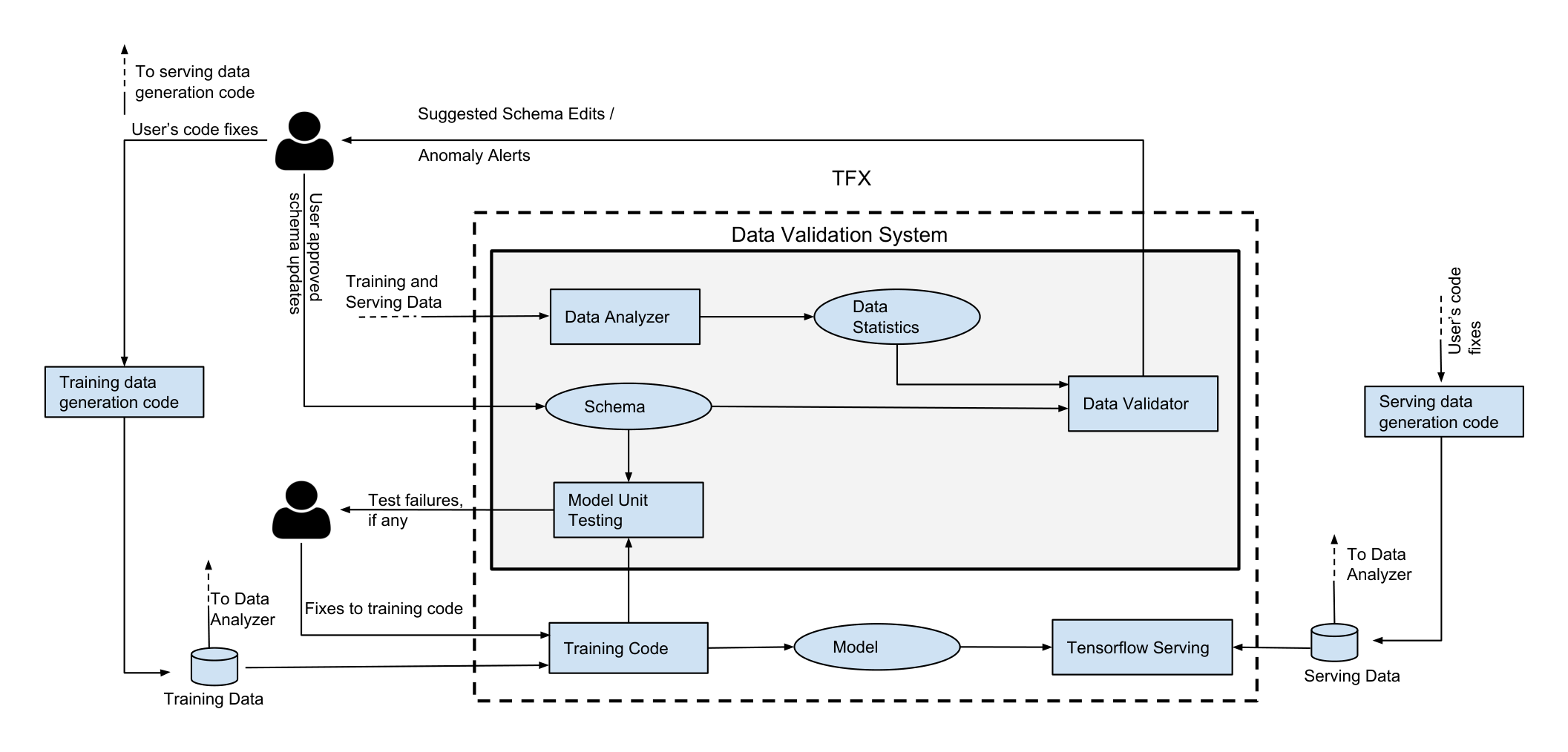
Figure 1 shows a schematic overview of our data-validation system and how it integrates with an end-to-end machine learning platform. At a high level, the platform instantiates a pipeline that ingests training data, passes it to data validation (our system), then pipes it to a training algorithm that generates a model, and finally pushes the latter to a serving infrastructure for inference. These pipelines typically work in a continuous fashion: a new batch of data arrives periodically, which triggers a new run of the pipeline. In other words, each batch of input data will trigger a new run of the data-validation logic and hence potentially a new set of data anomalies. Note that our notion of a batch is different than the mini-batches that constitute chunks of data used to compute and update model parameters during training. The batches of data ingested into the pipeline correspond to larger intervals of time (say a day). While our system supports validation of data on a sample of data ingested into the pipeline, this option is disabled by default since our current response times for single batch is acceptable for most users and within the expectations of end-to-end ML. Furthermore, by validating over the entire batch we ensure that anomalies that are infrequent or manifest in small but important slices of data are not silently ignored.

The data validation system consists of three main components – a Data Analyzer that computes predefined set of data statistics sufficient for data validation, a Data Validator that checks for properties of data as specified through a Schema (defined in Section 3), and a Model Unit Tester that checks for errors in the training code using synthetic data generated through the schema. Overall, our system supports the following types of data validation:

• Single-batch validation answers the question: are there any anomalies in a single batch of data? The goal here is to alert the on-call about the error and kick-start the investigation.
• Inter-batch validation answers the question: are there any significant changes between the training and serving data, or between successive batches of the training data? This tries to capture the class of errors that occur between software stacks (e.g., training data generation follows different logic than serving data generation), or to capture bugs in the rollout of new code (e.g., a new version of the training-data generation code results in different semantics for a feature, which requires old batches to be backfilled).
• Model testing answers the question: are there any assumptions in the training code that are not reflected in the data (e.g. are we taking the logarithm of a feature that turns out to be a negative number or a string?).

The following sections discuss the details of how our system performs these data validation checks and how our design choices address the challenges discussed in Section 1. Now, we acknowledge that these checks are not exhaustive, but our experience shows that they cover the vast majority of errors we have observed in production and so they provide a meaningful scope for the problem.

3 SINGLE-BATCH VALIDATION

Section Summary: This section explains how to detect errors in individual batches of data fed into machine learning pipelines, where each batch comes from a single run of code and should have consistent characteristics based on expert knowledge. To check this, the system uses a schema—a simple set of rules defining expected features like data types, ranges, and presence—that goes beyond basic formats to capture real-world meaning, such as distinguishing a person's age from a document's age. The validator compares batch statistics against the schema to flag anomalies early, alert teams, provide clear explanations, suggest updates for evolving data, and minimize false alarms through manual schema curation.

The first question we answer is: are there data errors within each new batch that is ingested by the pipeline?

We expect the data characteristics to remain stable within each batch, as the latter corresponds to a single run of the data-generation code. We also expect some characteristics to remain stable across several batches that are close in time, since it is uncommon to have frequent drastic changes to the data-generation code. For these reasons, we consider any deviation within a batch from the expected data characteristics, given expert domain knowledge, as an anomaly.

In order to codify these expected data characteristics, our system generalizes the traditional notion of a schema from database systems. The schema acts as a logical model of the data and attempts to capture some of the semantics that are lost when the data are transformed to the format accepted by training algorithms, which is typically key-value lists. To illustrate this, consider a training example with a key-value ("age", 150). If this feature corresponds to the age of a person in years then clearly there is an error. If, however, the feature corresponds to the age of a document in days then the value can be perfectly valid. The schema can codify our expectations for "age" and provide a reliable mechanism to check for errors.

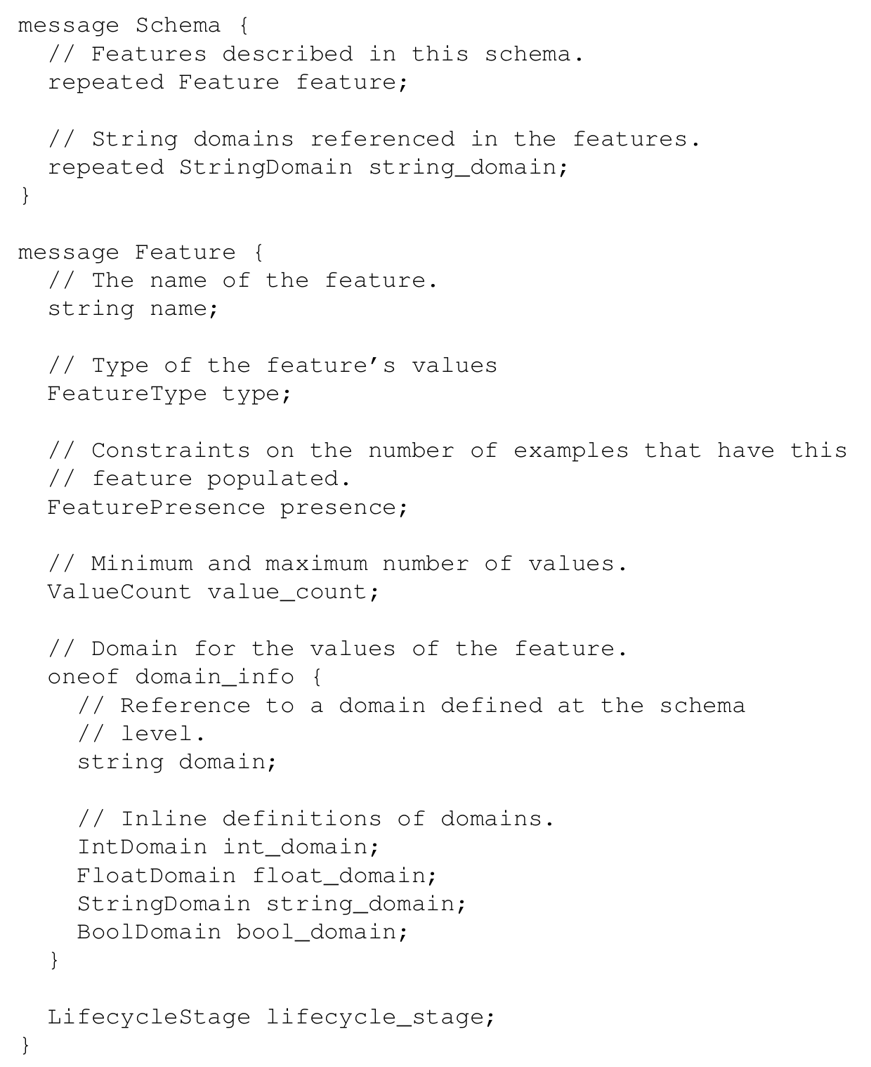
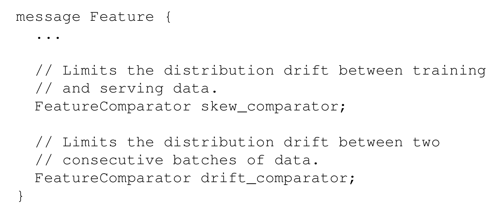
Figure 2 shows the schema formalism used by our data validation system, defined as a protocol buffer message (pro, 2017). (We use the protocol-buffer representation as it corresponds to our implementation and is also easy to follow.) The schema follows a logical data model where each training or serving example is a collection of features, with each feature having several constraints attached to it. This flat model has an obvious mapping to the flat data formats used by popular ML frameworks, e.g., tensorflow.Example or CSV. We have also extended the schema to cover structured examples (e.g., JSON objects or protocol buffers) but we do not discuss this capability in this paper.

The constraints associated with each feature cover some basic properties (e.g., type, domain, valency) but also constraints that are relevant to ML and that also reflect code-centric error patterns that we want to capture through data validation (see also our discussion in Section 1). For instance, the presence constraint covers bugs that cause the data-generation code to silently drop features from some examples (e.g., failed RPCs that cause the code to skip a feature). As another case, the domain constraints can cover bugs that change the representation of values for the same feature (e.g., a code-change that lower-cases the string representation of country codes for some examples). We defer a more detailed discussion of our schema formalism in Appendix A. However, we note that we do not make any claims on completeness – there are reasonable data properties that our schema cannot encode. Still, our experience so far has shown that the current schema is powerful enough to capture the vast majority of use cases in production pipelines.

Schema Validation The Data Validator component of our system validates each batch of data by comparing it against the schema. Any disagreement is flagged as an anomaly and triggers an alert to the on-call for further investigation. For now, we assume that the pipeline includes a user-curated schema that codifies all the constraints of interest. We discuss how to arrive at this state later.

In view of the design goals of data validation discussed in Section 1, the Data Validator component:

• attempts to detect issues as early in the pipeline as possible to avoid training on bad data. In order to ensure it can do so scalably and efficiently, we rely on the per-batch data statistics computed by a preceding Data Analyzer module. Our strategy of validating using these pre-computed statistics allows the validation itself to be fairly lightweight. This enables revalidation of the data using an updated schema near instantaneously.
• be easily interpretable and narrowly focused on the exact anomaly. Table 1 shows different categories of anomalies that our Data Validator reports to the user. Each anomaly corresponds to a violation of some property specified in the schema and has an associated description template that is populated with concrete values from the detected anomaly before being presented to the user.
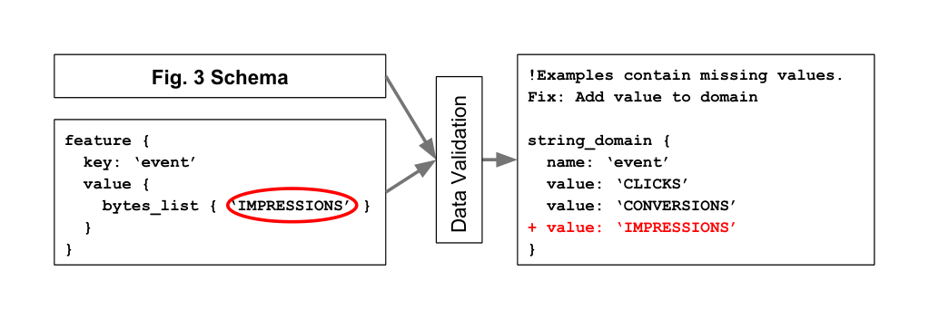
• include suggested updates to the schema to “eliminate” anomalies that correspond to the natural evolution of the data. For instance, as shown in Figure 4, the domain of “event” seems to have acquired a new IMPRESSIONS value, and so our validator generates a suggestion to extend the feature’s domain with the same value (this is shown with the red text and “+” sign in Figure 4).
• avoids false positives by focusing on the narrow set of constraints that can be expressed in our schema and by requiring that the schema is manually curated, thus ensuring that the user actually cares about the encoded constraints.

Schema Life Cycle As mentioned earlier, our assumption is that the pipeline owners are also responsible to curate the schema. However, many machine learning pipelines use thousands of features, and so constructing a schema manually for such pipelines can be quite tedious. Furthermore, the domain knowledge of the features may be distributed across a number of engineers within the product team or even outside of the team. In such cases, the upfront effort in schema construction can discourage engineers from setting up data validation until they run into a serious data error.

To overcome this adoption hurdle, the Data Validator component synthesizes a basic version of the schema based on all available batches of data in the pipeline. This auto-generated schema attempts to capture salient properties of the data without overfitting to a particular batch of data. Avoiding overfitting is important: an overfitted schema is more likely to cause spurious alerts when validating a new batch of data, which in turn increases the cognitive overhead for the on-call engineers, reduces their trust in the system, and may even lead them to switch off data validation altogether. We currently rely on a set of reasonable heuristics to perform this initial schema inference. A more formal solution, perhaps with guarantees or controls on the amount of overfitting, is an interesting direction for future work.

Once the initial schema is in place, the Data Validator will recommend updates to the schema as new data is ingested and analyzed. To help users manage the schema easily, our system also includes a user interface and tools that aid users by directing their attention to important suggestions and providing a click-button interface to apply the suggested changes. The user can then accept these suggested updates or manually edit the schema using her judgement. We expect owners of pipelines to treat the schema as a production asset at par with source code and adopt best practices for reviewing, versioning, and maintaining the schema. For instance, in our pipelines the schema is stored in the version-control system for source code.

4 INTER-BATCH VALIDATION

Section Summary: This section explains how anomalies in machine learning data can appear only when comparing multiple batches, such as shifts in feature values over time, and focuses on detecting "training-serving skew," where training data differs from real-time serving data due to varying processing methods. It breaks down three main types: feature skew, where individual features change values unexpectedly; distribution skew, where the overall spread of data varies between batches; and scoring/serving skew, where only some scored items are shown, creating feedback loops that bias future training. To catch these issues, tools like the Data Validator continuously compare samples using joins for features and distance metrics like KL divergence for distributions, while alerting users to potential problems without overly sensitive false alarms.

There are certain anomalies that only manifest when two or more batches of data are considered together, e.g., drift in the distribution of feature values across multiple batches of data. In this section, we first cover the different types of such anomalies, discuss the reasons why they occur, and finally present some common techniques that can be used to detect them.

Training-Serving Skew One of the issues that frequently occurs in production pipelines is skew between training and serving data. Several factors contribute to this issue but the most common is different code paths used for generation of training and serving data. These different code paths are required due to widely different latency and throughput characteristics of offline training data generation versus online serving data generation.

Based on our experience, we can broadly categorize training-serving skew into three main categories.

Feature skew occurs when a particular feature for an example assumes different values in training versus at serving time. This can happen, for instance, when a developer adds or removes a feature from the training-data code path but inadvertently forgets to do the same to the serving path. A more interesting mechanism through which feature skew occurs is termed time travel. This happens when the feature value is determined by querying a non-static source of data. For instance, consider a scenario where each example in our data corresponds to an online ad impression. One of the features for the impression is the number of clicks, obtained by querying a database. Now, if the training data is generated by querying the same database then it is likely that the click count for each impression will appear higher compared to the serving data, since it includes all the clicks that happened between when the data was served and when the training data was generated. This skew would bias the resulting model against a different distribution of click rates compared to what is observed at serving time, which is likely to affect model quality.

Distribution skew occurs when the distribution of feature values over a batch of training data is different from that seen at serving time. To understand why this happens consider the following scenario. Let us assume that we have a setup where a sample of today’s serving data is used as the training data for next day’s model. The sampling is needed since the volume of data seen at serving time is prohibitively large to train over. Any flaw in the sampling scheme can result in training data distributions that look significantly different from serving data distributions.

Scoring/Serving Skew occurs when only a subset of the scored examples are actually served. To illustrate this scenario, consider a list of ten recommended videos shown to the user out of hundred that are scored by the model. Subsequently if the user clicks on one of the ten videos, then we can treat that as a positive example and the other nine as negative examples for next day’s training. However, the ninety videos that were never served may not have associated labels and therefore may never appear in the training data. This establishes an implicit feedback loop which further increases the chances of misprediction for lower ranked items, and consequently less frequent appearance in training data. Detecting such types of skew is harder than the other two types.

In addition to validating individual batches of training data, the Data Validator also monitors for skew between training and serving data, continuously. Specifically, our serving infrastructure is configured to log a sample of the serving data which is imported back into the training pipeline. The Data Validator component continuously compares batches of incoming training and serving data to detect different types of skew. To detect feature skew, the Data Validator component does a key-join between corresponding batches of training and serving data followed by a feature wise comparison. Any detected skew is summarized and presented to the user using the ML platform’s standard alerting infrastructure. To detect distribution skew, we rely on measures that quantify the distance between distributions, which we discuss below. In addition to skew detection, each serving data batch is validated against the schema to detect the anomalies listed in Section 3. We note that in all cases, the parameters for skew detection are encoded as additional constraints in the schema.

Quantifying Distribution Distance As mentioned above, our distribution-skew detection relies on metrics that can quantify the distance between the training and serving distributions. It is important to note that, in practice, we expect these distributions to be different (and hence their distance to be positive), since the distribution of examples on each day is in fact different than the last. So the key question is whether the distance is high enough to warrant an alert.

A first-cut solution here might be to use typical distance metrics such as KL divergence or cosine similarity and fire an alert only if the metric crosses a threshold. The problem with this solution is that product teams have a hard time understanding the natural meaning of the metric and thus tuning the threshold to avoid false positives. Another approach might be to rely on statistical goodness-of-fit tests, where the alert can be tuned based on common confidence levels. For instance, one might apply a chi-square test and alert if the null hypothesis is rejected at the 1% confidence level. The problem with this general approach, however, is that the variance of test statistics typically has an inverse square relationship to the total number of examples, which makes these tests sensitive to even minute differences in the two distributions.

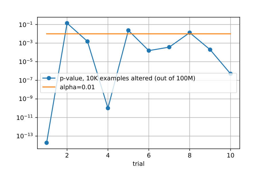
We illustrate the last point with a simple experiment. We begin with a control sample of 100 million points from a N(0,1) distribution and then randomly replace 10 thousand points by sampling from a N(0,2) distribution. This replacement introduces a minute amount of noise (0.01%) in the original data, for which ML is expected to be resilient. In other words, a human operator would consider the two distributions to be the “same”. We then perform a chi-square test between the two distributions to test their fit. Figure 5 shows the p-value of this test over 10 trials of this experiment, along with the threshold of 1% for the confidence level. Note that any p-value below the threshold implies that the test rejects the null hypothesis (that the two distributions are the same) and would therefore result in a distribution-skew alert. As shown, this method would needlessly fire an alert 7 out of 10 times and would most likely be considered a flaky detection method. We have repeated the same experiment with actual error-free data from one of our product teams and obtained qualitatively the same results.

To overcome these limitations we focus on distribution-distance metrics which are resilient to differences we observe in practice and whose sensitivity can be easily tuned by product teams. In particular, we use $d_{\infty}(p, q) = \max_{i \in S} |p_i - q_i|$ as the metric to compare two distributions $p$ and $q$ with probabilities $p_i$ and $q_i$ respectively for each value $i$ (from some universe). Notice that this metric has several desirable properties. First, it has a simple natural interpretation of the largest change in probability for a value in the two distributions, which makes it easier for teams to set a threshold (e.g., “allow changes of only up to 1% for each value”). Moreover, an alert comes with a “culprit” value that can be the starting point of an investigation. For instance, if the highest change in frequency is observed in value ’-1’ then this might be an issue with some backend failing and producing a default value. (This is an actual situation observed in one of our production pipelines.)

The next question is whether we can estimate the metric in a statistically sound manner based on observed frequencies. We develop a method to do that based on Dirichlet priors. For more details, see Appendix B.

5 MODEL UNIT TESTING

Section Summary: This section explains how machine learning platforms can encounter errors when custom training code makes hidden assumptions about data that aren't captured in the system's schema, such as expecting a feature to always be positive, which might work during training but cause crashes when serving the model with real data. To catch these issues early, the approach uses fuzz testing, generating random synthetic data that follows the schema to run the training code and reveal mismatches before they propagate. This method, while not perfect, effectively uncovers common errors with just a few hundred examples and has been integrated as a routine unit test in the platform to help users validate their training logic.

Up to this point, we focused on detecting mismatches between the expected and the actual state of the data. Our intent has been to uncover software errors in generating either training or serving data. Here, we shift gears and focus on a different class of software errors: mismatches between the expected data and the assumptions made in the training code. Specifically, recall that our platform (and similar platforms) allow the user to plug in their own training code to generate the model (see also Figure 1). This code is mostly a black box for the remaining parts of the platform, including the data-validation system, and can perform arbitrary computations over the data. As we explain below, these computations may make assumptions that do not agree with the data and cause serious errors that propagate through the ML infrastructure.

To illustrate this scenario, suppose that the training code applies a logarithm transform on a numeric feature, thus making the implicit assumption that the feature’s value is always positive. Now, let us assume that the schema does not encode this assumption (e.g., the feature’s domain includes non-positive values) and also that the specific instance of training data happens to carry positive values for this feature. As a result, two things happen: (a) data validation does not detect any errors, and (b) the generated model includes the same transform and hence the same assumption. Consider now what happens when the model is served and the serving data happens to have a non-positive value for the feature: the error is triggered, resulting in a (possibly crashing) failure inside the serving infrastructure.

The previous example illustrates the dangers of these hidden assumptions and the importance of catching them before they propagate through the served models. Note that the training code can make several other types of assumptions that are not reflected in the schema, e.g., that a feature is always present even though it is marked as optional, or that a feature has a dense shape even though it may take a variable number of values, to name a few that we have observed in production. Again, the danger of these assumptions is that they are not part of the schema (so they cannot be caught through schema validation) and they may be satisfied in the specific instance of training data (and so will not trigger during training).

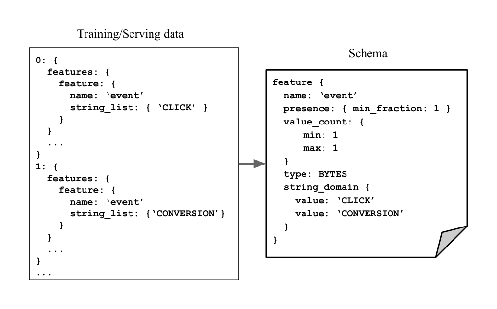
We base our approach on fuzz testing (Miller et al., 1990), using the schema to guide the generation of synthetic inputs. Specifically, we generate synthetic training examples that adhere to the schema constraints. For instance, if the schema in Figure 3 is used to generate data, each example will have an event feature, each of which would have one value, uniformly chosen at random to be either ‘CLICK’ or ‘CONVERSION’. Similarly, integral features would be random integers from the range specified in the schema, to name another case. The generation can be seeded so that it provides a deterministic output.

The generated data is then used to drive a few iterations of the training code. The goal is to trigger the hidden assumptions in the code that do not agree with the schema constraints. Returning to our earlier example with the logarithm transform, a synthetic input with non-positive feature values will cause an error and hence uncover the mismatch between the schema and the training code. At that point, the user can fix the training code, e.g., apply the transform on $max(value, 1)$, or extend the schema to mark the feature as positive (so that data validation catches this error). Doing both provides for additional robustness, as it enables alerts if the data violates the stated assumptions and protects the generated model from crashes if the data is wrong.

This fuzz-testing strategy is obviously not fool-proof, as the random data can still pass through the training code without triggering errors. In practice, however, we found that fuzz-testing can trigger common errors in the training code even with a modest number of randomly-generated examples (e.g., in the 100s). In fact, it has worked so well that we have packaged this type of testing as a unit test over training algorithms, and included the test in the standard templates of our ML platform. Our users routinely execute these unit tests to validate changes to the training logic of their pipelines. To our knowledge, this application of unit testing in the context of ML and for the purpose of data validation is a novel aspect of our work.

6 EMPIRICAL VALIDATION

Section Summary: The data-validation system has been successfully deployed in a large organization's machine learning platform, processing petabytes of data daily and saving significant engineer time by detecting anomalies early to prevent faulty models and aiding in troubleshooting data-related issues. Analysis of over 700 pipelines shows that schemas evolve alongside data, with most undergoing a few updates to reflect natural changes, indicating that data shifts steadily rather than unpredictably and encouraging teams to treat schemas as key documentation tools. Common anomalies, such as new or missing features and unexpected values, occur in about 10% of pipelines but are fixed in over half the cases, demonstrating the system's effectiveness in prompting timely resolutions.

As mentioned earlier, our data-validation system has been deployed in production as part of the standard ML platform used in a large organization. The system currently analyzes several petabytes of training and serving data per day and has resulted in significant savings in engineer hours in two ways: by catching important data anomalies early (before they result in a bad model being pushed to production), and by helping teams diagnose model-quality problems caused by data errors. In what follows we provide empirical evidence to back this claim. We first report aggregate results from our production deployment and then discuss in some detail individual use cases.

6.1 Results from Production Deployment

We present an analysis of our system in production, based on a sample of more than 700 ML pipelines that employ data validation and train models that are pushed to our production serving infrastructure.

We first consider the co-evolution of data and schema in the lifecycle of these pipelines, which is a core tenet of our approach. Recall that our users go through the following workflow: (i) when the pipeline is set up, they obtain an initial schema through our automatic inference, (ii) they review and manually edit the schema to compensate for any missing domain knowledge, (iii) they commit the updated schema to a version control system and start the training part of the pipeline. Subsequently, when a data alert fires that indicates a disagreement between the data and the schema, the user has the option to either fix the data generation process or update the schema, if the alert corresponds to a natural evolution of the data. Here we are interested in understanding the latter changes that reflect the co-evolution we mentioned.

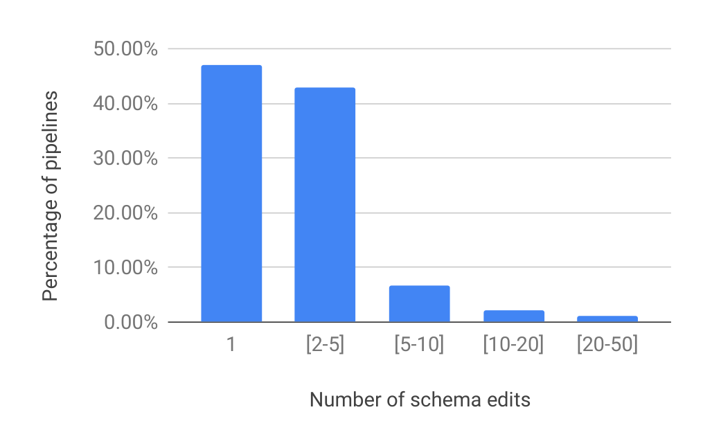
Figure 6 shows a histogram of this number of schema changes across the >700 pipelines that we considered. The graph illustrates that the schema evolves in most of the examined pipelines, in line with our hypothesis of data-schema co-evolution.

The majority of cases have up to five schema revisions, with the distribution tapering off after that point. This evidence suggests that the input data has evolving properties but is not completely volatile, which is reasonable in practice. On the side, we also conclude that the engineers treat the schema as an important production asset and hence are willing to put in the effort to keep it up to date. In fact, anecdotal evidence from some teams suggest a mental shift towards a data-centric view of ML, where the schema is not solely used for data validation but also provides a way to document new features that are used in the pipeline and thus disseminate information across the members of the team.

In our next analysis we examine in more detail how users interact with the schema. Specifically, we instrumented our system to monitor the types of data anomalies raised in production and the subsequent reactions of the users in terms of schema updates. Table 1 summarizes the results. As shown, the most common anomalies are new feature columns, unexpected string values, and missing feature columns. The first two are unsurprising: even in a healthy pipeline, there will be new values for fields such as “postal code”, and new feature columns are constantly being created by feature engineers. Missing features and missing data are more cause for concern. We can see from the chart that it is very rare that the physical type of a feature column is wrong (for example, someone manually added a feature column with the wrong type, causing this anomaly); nonetheless, by checking this we check agreement between the prescriptive nature of the schema and the actual data on disk. Even in cases where the anomalies almost never fire, this check is useful.

: Table 1: Analysis of data anomalies over the most recent 30-day period for evaluation pipelines. First, we checked the schemas, to determine what fraction of pipelines could possibly fire a particular kind of alert (Used). Then, we looked at each day, and saw what kinds of anomalies Fired, and calculated what fraction of pipelines had an anomaly fire on any day. If there were two days with none of this type of anomaly firing on a pipeline afterward, then we considered the problem Fixed. This methodology can miss some fixes, if an anomaly is fixed but a new anomaly of the same type arrives the next day. It is also possible that an anomaly appears fixed but wasn’t if a pipeline stopped or example validation was turned off, but this is less likely.

\begin{tabular}{|p{4.5cm}|c|c|c|}
\hline
Anomaly Category & Used & Fired & Fixed given Fired \\
\hline
New feature column (in data but not in schema) & 100\% & 10\% & 65\% \\
Out of domain values for categorical features & 45\% & 6\% & 66\% \\
Missing feature column (in schema but not in data) & 97\% & 6\% & 53\% \\
The fraction of examples containing a feature is too small & 97\% & 3\% & 82\% \\
Too small feature value vector for example & 98\% & 2\% & 56\% \\
Too large feature value vector for example & 98\% & <1\% & 28\% \\
Data completely missing & 100\% & 3\% & 65\% \\
Incorrect data type for feature values & 98\% & <1\% & 100\% \\
Non-boolean value for boolean feature type & 14\% & <1\% & 100\% \\
Out of domain values for numeric features & 67\% & 1\% & 77\% \\
\hline
\end{tabular}

Table 1 also shows that product teams fix the majority of the detected anomalies. Now, some anomalies remain unfixed and we postulate that this happens for two reasons. First, in some cases a reasonable course of action is to let the anomalous batch slide out of the pipeline’s rolling window, e.g., in the case of a data-missing anomaly where regenerating the data is impossible. Second, as we mentioned repeatedly, we are dealing with a human operator in the loop who might miss or ignore the alert depending on their cognitive load. This re-emphasizes the observation that we need to be mindful of how and when we deliver the anomaly alerts to the on-call operators.

Finally, we turn our attention to the data-validation workflow through model unit testing. Again, this unit testing is part of the standard ML platform in our organization and so we were able to gather fleet-wide statistics on this functionality. Specifically, more than 70% of pipelines had at least one model unit test defined. Based on analysis of test logs over a period of one month, we determined that these tests were executed more than 80K times (including runs executed as part of continuous test framework). Of all of these executions 6% had failures indicating that either the training code had incorrect assumptions about the data or the schema itself was under specified.

6.2 Case Studies

In addition to the previous results, we present three case studies that illustrate the benefits of our system in production.

Missing features in Google Play recommender pipeline. The goal of the Google Play recommender system is to recommend relevant Android apps to the Play app users when they visit the homepage of the store, with an aim of driving discovery of apps that will be useful to the user. Using the Data Validation system of TFX, Google Play discovered a few features that were always missing from the logs, but always present in training. The results of an online A/B experiment showed that removing this skew improved the app install rate on the main landing page of the app store by 2%.

Data debugging leads to model wins. One of the product teams in our organization employs ML to generate video recommendations. The product team needed to migrate their existing training and serving infrastructure onto the new ML platform that also includes data validation. A prerequisite for the migration was of course to achieve parity in terms of model quality. After setting up the new infrastructure, our data-validation system started generating alerts about missing features over the serving data. During the ensuing investigation, the team discovered that a backend system was storing some features in a different format than expected which caused these features to be silently dropped in their data-parsing code. In this case, the hard part was identifying the features which exhibited the problem (and this is precisely the information provided by our data-validation service)– the fix was easy and resulted in achieving performance parity. The total time to diagnose and fix the problem was two days, whereas similar issues have taken months to resolve.

Stand-alone data validation. Some product teams are setting up ML pipelines solely for the purpose of running our data-validation system, without doing any training or serving of models. These teams have existing infrastructure (predating the ML platform) to train and serve models, but they are lacking a systematic mechanism for data validation and, as a result, they are suffering from the data-related issues that we described earlier in the paper. To address this shortcoming in their infrastructure, these teams have set up pipelines that solely monitor the training and serving data and alert the on-call when an error is detected (while training and serving still happen using the existing infrastructure).

Feature-store migration. Two product teams have used our system to validate the migration of their features to new stores. In this setup, our system was used to apply schema validation and drift detection on datasets from the old and new storage systems, respectively. The detected data errors helped the teams debug the new storage system and consequently complete the migration successfully.

7 RELATED WORK

Section Summary: This section compares the authors' Google-deployed machine learning system to Amazon's more flexible approach, highlighting their choice of a simpler schema language for easier management and a focus on evolving data schemas alongside models with user input. It situates the work within broader efforts to build complete machine learning platforms that handle everything from data to serving and monitoring, but emphasizes their detailed emphasis on validating production data, contrasting with general overviews in prior research. Related topics like data cleaning tools that fix errors, schema creation in databases, skew detection via interpretable metrics, and model testing through generated examples are discussed, noting how this system's data-driven alerts and ML-specific constraints set it apart.

As compared to a similar system from Amazon (Schelter et al., 2018), our design choices and techniques are informed based on wide deployment of our system at Google. While Amazon’s system allows users to express arbitrary constraints, we opted to have a restrictive schema definition language that captures the data constraints for most of our users while permitting us to develop effective tools to help users manage their schema. Another differentiating factor of our work is the emphasis on co-evolution of the schema with data and the model with the user in the loop.

While model training (Abadi et al., 2016; ker; mxn) is a central topic, it is only one component of a machine learning platform and represents a small fraction of the code (Sculley et al., 2015). As a result, there is an increasing effort to build end-to-end machine learning systems (Chandra, 2014; Baylor et al., 2017; Sparks et al., 2017; Bose et al., 2017) that cover all aspects of machine learning including data management (Polyzotis et al., 2017), model management (Vartak, 2017; Fernandez et al., 2016; Schelter et al., 2017), and model serving (Olston et al., 2017; Crankshaw et al., 2015), to name a few. In addition, testing and monitoring are necessary to reduce technical debt and ensure product readiness of machine learning systems (Breck et al., 2017). In comparison, this paper specifically focuses on data validation for production machine learning. In addition we go into detail on a particular solution to the problem, compared to previous work that covered in broad strokes the issues related to data management and machine learning (Polyzotis et al., 2017).

A topic closely related to data validation is data cleaning (Rekatsinas et al., 2017; Stonebraker et al., 2013; Khayyat et al., 2015; Volkovs et al., 2014) where the state-of-art is to incorporate multiple signals including integrity constraints, external data, and quantitative statistics to repair errors. More recently, several cleaning tools target machine learning. BoostClean (Krishnan et al., 2017) selectively cleans out-of-range errors that negatively affect model accuracy. Data linter (Hynes et al., 2017) uses best practices to identify potential issues and efficiencies of machine learning data. In comparison, our system uses a data-driven schema utilizing previous data to generate actionable alerts to users. An interesting direction is to perform root cause analysis (Wang et al., 2015) that is actionable as well.

Schema generation is commonly done in Database systems (DiScala & Abadi, 2016) where the main focus is on query processing. As discussed in Section 1, our context is unique in that the schema is reverse-engineered and has to co-evolve with the data. Moreover, we introduce schema constraints unique to ML.

Skew detection is relevant to various statistical approaches including homogeneity tests (Pearson, 1992), analysis of variance (Fisher, 1921; 1992), and time series analysis (Basseville & Nikiforov, 1993; Ding et al., 2008; Brodersen et al., 2015). As discussed, our approach is to avoid statistical tests that lead to false positive alerts and instead rely on more interpretable metrics of distribution distance, coupled with sound approximation methods.

The traditional approach of model testing is to select a random set of examples from manually labeled datasets (Witten et al., 2011). More recently, adversarial deep learning techniques (Goodfellow et al., 2014) have been proposed to generate examples that fool deep neural networks. DeepXplore (Pei et al., 2017) is a whitebox tool for generating data where models make different predictions. There are also many tools for traditional software testing. In comparison, our model testing uses a schema to generate data and can thus work for any type of models. The process of iteratively adjusting the schema is similar in spirit to version spaces (Russell & Norvig, 2009) and has connections with teaching learners (Frazier et al., 1996).

REFERENCES

Section Summary: This references section lists a variety of sources used in the document, including websites for popular machine learning frameworks like Keras, MXNet, and TensorFlow, which provide tools for building and training AI models. It also includes numerous academic papers from conferences and journals, covering topics such as large-scale machine learning systems, data quality verification, probabilistic forecasting, and automated error detection in datasets. These citations draw from experts and organizations like Google, drawing on research from the 1990s to 2018 to support discussions on practical AI applications and challenges.

Keras. https://keras.io/.

Mxnet. https://mxnet.incubator.apache.org/.

Tensorflow examples. https://www.tensorflow.org/programmers\_guide/datasets.

Protocol buffers. https://developers.google.com/protocol-buffers/, 2017.

Abadi, M., Barham, P., Chen, J., Chen, Z., Davis, A., Dean, J., Devin, M., Ghemawat, S., Irving, G., Isard, M., Kudlur, M., Levenberg, J., Monga, R., Moore, S., Murray, D. G., Steiner, B., Tucker, P., Vasudevan, V., Warden, P., Wicke, M., Yu, Y., and Zheng, X. Tensorflow: A system for large-scale machine learning. In OSDI, pp. 265–283, 2016. ISBN 978-1-931971-33-1.

Basseville, M. and Nikiforov, I. V. Detection of Abrupt Changes: Theory and Application. Prentice-Hall, Inc., 1993. ISBN 0-13-126780-9.

Baylor, D., Breck, E., Cheng, H.-T., Fiedel, N., Foo, C. Y., Haque, Z., Haykal, S., Ispir, M., Jain, V., Koc, L., Koo, C. Y., Lew, L., Mewald, C., Modi, A. N., Polyzotis, N., Ramesh, S., Roy, S., Whang, S. E., Wicke, M., Wilkiewicz, J., Zhang, X., and Zinkevich, M. TFX: A tensorflow-based production-scale machine learning platform. In SIGKDD, pp. 1387–1395, 2017. ISBN 978-1-4503-4887-4. doi: 10.1145/3097983.3098021. URL http://doi.acm.org/10.1145/3097983.3098021.

Bose, J.-H., Flunkert, V., Gasthaus, J., Januschowski, T., Lange, D., Salinas, D., Schelter, S., Seeger, M., and Wang, Y. Probabilistic demand forecasting at scale. PVLDB, 10 (12):1694–1705, August 2017. ISSN 2150-8097.

Breck, E., Cai, S., Nielsen, E., Salib, M., and Sculley, D. The ml test score: A rubric for ml production readiness and technical debt reduction. In IEEE Big Data, 2017.

Brodersen, K. H., Gallusser, F., Koehler, J., Remy, N., and Scott, S. L. Inferring causal impact using bayesian structural time-series models. Annals of Applied Statistics, 9: 247–274, 2015.

Chandra, T. Sibyl: a system for large scale machine learning at Google. In Dependable Systems and Networks (Keynote), Atlanta, GA, 2014. URL http://www.youtube.com/watch?v=3SaZ5UAQrQM.

Crankshaw, D., Bailis, P., Gonzalez, J. E., Li, H., Zhang, Z., Franklin, M. J., Ghodsi, A., and Jordan, M. I. The missing piece in complex analytics: Low latency, scalable model management and serving with velox. In CIDR, 2015. URL http://cidrdb.org/cidr2015/Papers/CIDR15\_Paper19u.pdf.

Ding, H., Trajcevski, G., Scheuermann, P., Wang, X., and Keogh, E. Querying and mining of time series data: Experimental comparison of representations and distance measures. PVLDB, 1(2):1542–1552, August 2008. ISSN 2150-8097. doi: 10.14778/1454159.1454226. URL http://dx.doi.org/10.14778/1454159.1454226.

DiScala, M. and Abadi, D. J. Automatic generation of normalized relational schemas from nested key-value data. In SIGMOD, pp. 295–310, 2016. ISBN 978-1-4503-3531-7.

Fernandez, R. C., Abedjan, Z., Madden, S., and Stonebraker, M. Towards large-scale data discovery: Position paper. In ExploreDB, pp. 3–5, 2016. ISBN 978-1-4503-4312-1.

Fisher, R. A. On the probable error of a coefficient of correlation deduced from a small sample. Metron, 1: 3–32, 1921.

Fisher, R. A. Statistical Methods for Research Workers, pp. 66–70. Springer-Verlag New York, 1992.

Frazier, M., Goldman, S. A., Mishra, N., and Pitt, L. Learning from a consistently ignorant teacher. J. Comput. Syst. Sci., 52(3):471–492, 1996. doi: 10.1006/jcss.1996.0035. URL https://doi.org/10.1006/jcss.1996.0035.

Frigyik, B. A., Kapila, A., and Gupta, M. R. Introduction to the dirichlet distribution and related processes. Technical report, University of Washington Department of Electrical Engineering, 2010. UWEETR-2010-0006.

Goodfellow, I. J., Shlens, J., and Segedy, C. Explaining and harnessing adversarial examples. CoRR, abs/1412.6572, 2014. URL http://arxiv.org/abs/1412.6572.

Hynes, N., Scully, D., and Terry, M. The data linter: Lightweight, automated sanity checking for ml data sets. In Workshop on ML Systems at NIPS 2017, 2017.

Khayyat, Z., Ilyas, I. F., Jindal, A., Madden, S., Ouzzani, M., Papotti, P., Quiane-Ruiz, J.-A., Tang, N., and Yin, S. Bigdansing: A system for big data cleansing. In SIGMOD, pp. 1215–1230, 2015.

Krishnan, S., Franklin, M. J., Goldberg, K., and Wu, E. Boostclean: Automated error detection and repair for machine learning. CoRR, abs/1711.01299, 2017. URL http://arxiv.org/abs/1711.01299.

Miller, B. P., Fredriksen, L., and So, B. An empirical study of the reliability of unix utilities. Commun. ACM, 33 (12):32–44, December 1990. ISSN 0001-0782. doi: 10.1145/96267.96279. URL http://doi.acm.org/10.1145/96267.96279.

Olston, C., Li, F., Harmsen, J., Soyke, J., Gorovoy, K., Lao, L., Fiedel, N., Ramesh, S., and Rajashekhar, V. Tensorflow-serving: Flexible, high-performance ml serving. In Workshop on ML Systems at NIPS 2017, 2017.

Pearson, K. On the Criterion that a Given System of Deviations from the Probable in the Case of a Correlated System of Variables is Such that it Can be Reasonably Supposed to have Arisen from Random Sampling, pp. 11–28. Springer-Verlag New York, 1992.

Pei, K., Cao, Y., Yang, J., and Jana, S. Deepxplore: Automated whitebox testing of deep learning systems. In SOSP, pp. 1–18, 2017. ISBN 978-1-4503-5085-3.

Polyzotis, N., Roy, S., Whang, S. E., and Zinkevich, M. Data management challenges in production machine learning. In SIGMOD, pp. 1723–1726, 2017.

Rekatsinas, T., Chu, X., Ilyas, I. F., and Ré, C. Holoclean: Holistic data repairs with probabilistic inference. PVLDB, 10(11):1190–1201, August 2017. ISSN 2150-8097.

Russell, S. and Norvig, P. Artificial Intelligence: A Modern Approach. Prentice Hall Press, Upper Saddle River, NJ, USA, 3rd edition, 2009. ISBN 0136042597, 9780136042594.

Schelter, S., Boese, J.-H., Kirschnick, J., Klein, T., and Seufert, S. Automatically tracking metadata and provenance of machine learning experiments. In Workshop on ML Systems at NIPS 2017, 2017.

Schelter, S., Lange, D., Schmidt, P., Celikel, M., Biessmann, F., and Grafberger, A. Automating large-scale data quality verification. Proc. VLDB Endow., 11(12): 1781–1794, August 2018. ISSN 2150-8097. doi: 10.14778/3229863.3229867. URL https://doi.org/10.14778/3229863.3229867.

Sculley, D., Holt, G., Golovin, D., Davydov, E., Phillips, T., Ebner, D., Chaudhary, V., Young, M., Crespo, J.-F., and Dennison, D. Hidden technical debt in machine learning systems. In NIPS, pp. 2503–2511, 2015. URL http://dl.acm.org/citation.cfm?id=2969442.2969519.

Sparks, E. R., Venkataraman, S., Kaftan, T., Franklin, M. J., and Recht, B. Keystoneml: Optimizing pipelines for large-scale advanced analytics. In ICDE, pp. 535–546, 2017.

Stonebraker, M., Bruckner, D., Ilyas, I. F., Beskales, G., Cherniack, M., Zdonik, S. B., Pagan, A., and Xu, S. Data curation at scale: The data tamer system. In CIDR, 2013.

Vartak, M. MODELDB: A system for machine learning model management. In CIDR, 2017.

Volkovs, M., Chiang, F., Szlichta, J., and Miller, R. J. Continuous data cleaning. In ICDE, pp. 244–255, 2014. doi: 10.1109/ICDE.2014.6816655.

Wang, X., Dong, X. L., and Meliou, A. Data x-ray: A diagnostic tool for data errors. In SIGMOD, pp. 1231–1245, 2015. ISBN 978-1-4503-2758-9. doi: 10.1145/2723372.2750549. URL http://doi.acm.org/10.1145/2723372.2750549.

Witten, I. H., Frank, E., and Hall, M. A. Data Mining: Practical Machine Learning Tools and Techniques. Morgan Kaufmann Publishers Inc., San Francisco, CA, USA, 3rd edition, 2011. ISBN 0123748569, 9780123748560.

A CONSTRAINTS IN THE DATA SCHEMA

Section Summary: The section describes constraints in a data schema designed to ensure consistency in machine learning features, starting with basics like data types (such as integers, floats, or bytes), which must remain stable to avoid errors in training models. It also covers expectations for feature presence in data examples, the number of values per feature (single or variable-length lists), restricted value domains that can include semantic meanings beyond raw types, and lifecycle stages for features, from experimental to production, which influence how seriously anomalies are treated. Additional advanced constraints, like logical sequences or value distributions, are mentioned but not fully detailed here.

We explain some of these feature level characteristics below using an instance of the schema shown in Figure 3:

Feature type: One of the key invariants of a feature is its data type. For example, a change in the data type from integer to string can easily cause the trainer to fail and is therefore considered a serious anomaly. Our schema allows specification of feature types as INT, FLOAT, and BYTES, which are the allowed types in the tf.train.Example (tfe) format. In Figure 3, the feature “event” is marked as of type BYTES. Note that features may have richer semantic types, which we capture in a different part of the schema (explained later).

Feature presence: While some features are expected to be present in all examples, others may only be expected in a fraction of the examples. The FeaturePresence field can be used to specify this expectation of presence. It allows specification of a lower limit on the fraction of examples that the feature must be present. For instance, the property presence: {min_fraction: 1} for the “event” feature in Figure 3 indicates that this feature is expected to be present in all examples.

Feature value count: Features can be single valued or lists. Furthermore, for features that are lists, they may or may not all be of the same length. These value counts are important to determine how the values can be encoded into the low-level tensor representation. The ValueCount field in the schema can be used to express such properties. In the example in Figure 3, the feature “event” is indicated to be a scalar as expressed using the min and max values set to 1.

Feature domains: While some features may not have a restricted domain (for example, a feature for “user queries”), many features assume values only from a limited domain. Furthermore, there may be related features that assume values from the same domain. For instance, it makes sense for two features like “apps_installed” and “apps_used” to be drawn from the same set of values. Our schema allows specification of domains both at the level of individual features as well as at the level of the schema. The named domains at the level of schema can be shared by all relevant features. Currently, our schema only supports shared domains for features with string domains.

A domain can also encode the semantic type of the data, which can be different than the raw type captured by the TYPE field. For instance, a bytes features may use the values “TRUE” or “FALSE” to essentially encode a boolean feature. Another example is an integer feature encoding categorical ids (e.g., enum values). Yet another example is a bytes feature that encodes numbers (e.g., values of the sort “123”). These patterns are fairly common in production and reflect common practices in translating structured data into the flat tf.train.Example format. These semantic properties are important for both data validation and understanding, and so we allow them to be marked explicitly in the domain construct of each feature.

Feature life cycle: The feature set used in a machine learning pipeline keeps evolving. For instance, initially a feature may be introduced only for experimentation. After sufficient trials, it may be promoted to a beta stage before finally getting upgraded to be a production feature. The gravity of anomalies in the features at different stages is different. Our schema allows tagging of features with the stage of life cycle that they are currently in. The current set of stages supported are UNKNOWN_STAGE, PLANNED, ALPHA, BETA, PRODUCTION, DEPRECATED, and DEBUG_ONLY.

Figure 2 only shows only a fragment of the constraints that can be expressed by our schema. For instance, our schema can encode how groups of features can encode logical sequences (e.g., the sequence of queries issued by a user where each query can be described with a set of features), or can express constraints on the distribution of values over the feature’s domain. We will cover some of these extensions in Section 4, but we omit a full presentation of the schema in the interest of space.

B STATISTICAL SIGNIFICANCE OF MEASUREMENTS OF DRIFT

Section Summary: This section explores how to determine if differences, or "drift," between two sets of data observations are reliable, rather than just random noise, by comparing their distributions statistically. It distinguishes between empirical drift, based directly on observed data, and theoretical drift, estimated using Bayesian methods with a Dirichlet prior to sample underlying probabilities and compute distances like the L1 metric, which sums absolute differences and reflects visual distinguishability. For massive datasets with billions of observations and fewer than 100 categories, the empirical drift closely matches the theoretical one, and the L1 approach is valuable because it highlights impacts on a broad number of examples, unlike metrics sensitive to rare events.

Suppose that we have two days of data, and we have some measure of their distance? As we discussed in Section 4, this measure will never be zero, as some real drift is always expected. However, how do we know if we can trust such a measurement?

Specifically, suppose that there is a set $S$ where $|S| = n$ of distinct observations we can make, and $\Delta(S)$ is the set of all distributions over $S$. Without loss of generality, we assume $S = {1 \dots n}$. In one dataset, there are $m_p$ observations $P_1 \dots P_{m_p} \in S$ with an empirical distribution $\hat{p} = \hat{p}_1 \dots \hat{p}n$. In a second dataset, there are $m_q$ observations $Q_1 \dots Q{m_q}$ with an empirical distribution $\hat{q} = \hat{q}1 \dots \hat{q}n$. We can assume that the elements in $P_1 \dots P{m_p}$ were drawn independently from some distribution $p = p_1 \dots p_n$, that was in turn drawn from a fixed Dirichlet prior (Frigyik et al., 2010) $Dir(\alpha)$ where $\alpha = (1 \dots 1)$ (a uniform density over the simplex), and similarly, $Q_1 \dots Q{m_q}$ were drawn independently from some distribution $q = q_1 \dots q_n$, that was in turn drawn from the same fixed Dirichlet prior.

If we have a particular measure $d : \Delta(S) \times \Delta(S) \rightarrow \mathbf{R}$, we have two options. First, we could measure the empirical drift $d(\hat{p}, \hat{q})$. Or we could attempt to estimate the theoretical drift $d(p, q)$. Although $p$ and $q$ are not directly observed, the latter can be achieved more easily than one might expect. First of all, the posterior distribution over $p$ given the observations $P_1 \dots P_{m_p}$ is simply $Dir(\alpha + m_p\hat{p})$, and the posterior distribution of $q$ is $Dir(\alpha + m_q\hat{q})$ (see Section 1.2 in (Frigyik et al., 2010)). Thus, one can get a sample from the posterior distribution of $d(p, q)$ by sampling $p'$ from $Dir(\alpha + m_p\hat{p})$ (see Section 2.2 in (Frigyik et al., 2010)) and $q'$ from $Dir(\alpha + m_q\hat{q})$ and calculating $d(p', q')$.

One metric we use is $d_1(p, q) = \sum_{i=1}^n |p_i - q_i|$. The advantage of $d_1$ is that it corresponds to how visually distinguishable two distributions are (see Figure 8). Consider a field that has 100 values that are all equally likely. If all values are uppercase instead of lowercase, then the $d_{\infty}(p, q) = 0.01$, but $d_1(p, q) = 1$ (the highest possible value).

What we find, if estimate the theoretical drift as described above, is that when $m_p$ and $m_q$ are at least a billion and $n < 100$, then $d(p, q)$ is very close to $d(\hat{p}, \hat{q})$. In other words, for the datasets that we care about, the empirical drift $d_{\infty}(\hat{p}, \hat{q})$ is a sound approximation of the theoretical drift.

Moreover, the empirical drift of $d_1$ can be visualized:

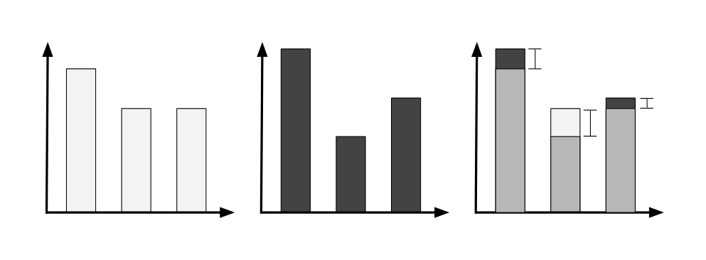
The connection to visualization is important: for instance, if we observe a high KL divergence, Kolmogorov-Smirnov statistic, or a low cosine similiarity, it is likely that the first thing a human will do is look at the two distributions and visually inspect them. The scenarios where the L1 distance is low but the KL divergence is high correspond to when very small probabilities ($10^{-6}$) become less small ($10^{-3}$). It is unclear whether such small fluctuations on the probability of rare features are cause for concern in general, whereas the magnitude of $d_1$ directly corresponds to the number of examples impacted, which in turn can affect performance.