Learning Convolutional Neural Networks for Graphs

Mathias NiepertMohamed AhmedKonstantin Kutzkov

article2016ICML2,300 citations

Develops a general framework for applying convolutional neural networks directly to arbitrary graphs by extracting and ordering local neighborhood subgraphs, matching graph kernel classification performance with greater computational efficiency.

Listen

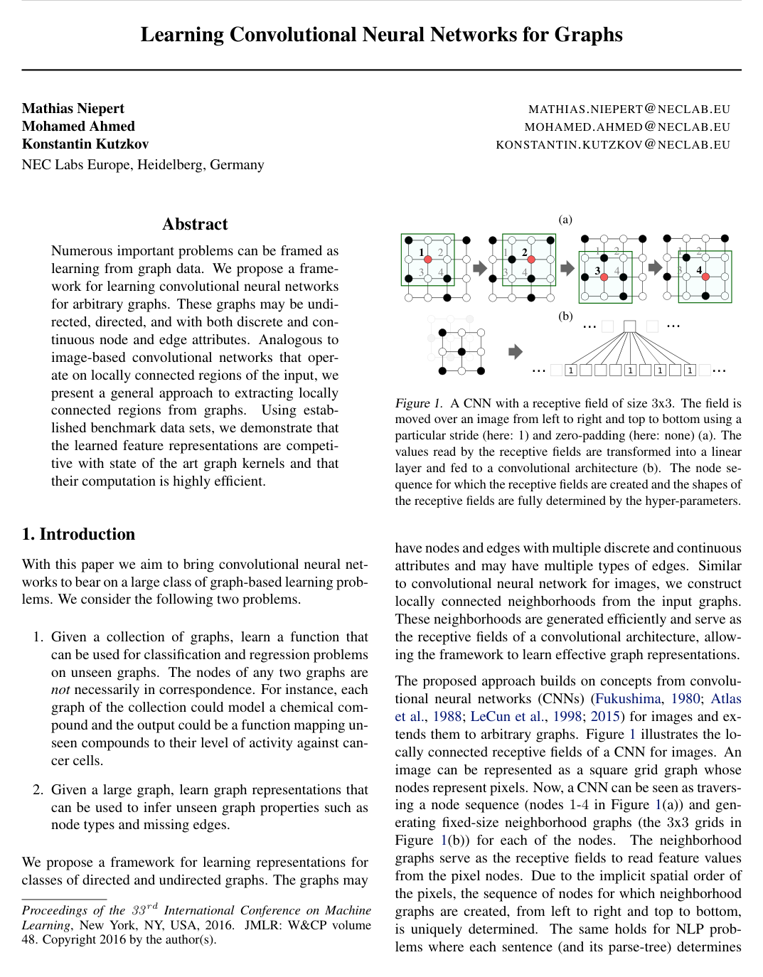
Many critical real-world applications—ranging from drug discovery and bioinformatics to social network analysis—rely on analyzing complex data structured as arbitrary graphs. While convolutional neural networks (CNNs) have delivered transformative breakthroughs in computer vision and natural language processing, they historically depend on rigid spatial grids or linear orders, making them difficult to apply directly to arbitrary graphs lacking a natural node alignment or ordering.

The article sets out to design, formalize, and evaluate PATCHY-SAN, a general framework that enables standard convolutional neural networks to learn representations from arbitrary directed, undirected, and attributed graphs without requiring manual feature engineering.

To evaluate this framework, the authors implemented a four-step pipeline that selects key node sequences, extracts local neighborhoods, normalizes these subgraphs into ordered vector patches using graph labeling procedures (such as the Weisfeiler-Lehman algorithm), and feeds them into standard convolutional neural network architectures. The authors tested this approach against established baseline graph kernels across multiple real-world benchmark datasets, including chemical compounds (MUTAG, PTC, NCI1), protein structures (PROTEIN, D&D), and large-scale social networks comprising up to 12,000 graphs.

The experimental findings show that PATCHY-SAN achieves classification accuracy competitive with or superior to state-of-the-art graph kernels. On social network benchmarks, the model significantly outperformed existing methods, improving classification accuracy by roughly 8 to 9 percentage points on key datasets (such as RE-B and RE-M5k). Computationally, the framework proved between 2 and 8 times faster than the fastest baseline graph kernel (Weisfeiler-Lehman), maintaining high patch-generation throughput (over 1,000 receptive fields per second for standard sizes) capable of saturating downstream deep learning pipelines. In addition, the framework easily handles continuous node and edge attributes and scales linearly with the number of input graphs, whereas classical graph kernels scale quadratically.

These results demonstrate that deep learning can be effectively applied to graph-structured domains without handcrafting specialized graph kernels. For organizations handling large collections of molecular or network data, this approach substantially reduces computational overhead, cuts processing time from days to seconds on large datasets, and enhances classification accuracy.

Organizations analyzing relational or graph-structured datasets should consider adopting localized receptive-field extraction to deploy standard convolutional neural network workflows. For future development, the authors suggest exploring alternative network backbones such as recurrent neural networks, evaluating multi-scale receptive field sizes, and incorporating unsupervised pretraining methods like autoencoders.

The primary limitations noted in the article include increased variance in small datasets when using untuned global hyperparameters, as well as the theoretical worst-case exponential complexity of exact graph canonicalization, although localized bounding keeps typical execution highly efficient in practice.

NEC Laboratories Europe bipartite graphs convolutional neural networks directed graphs convolutional neural networks for graphs deep graph kernels graph sequence neural networks

arXiv: 1605.05273

Paper: Spectral Networks and Locally Connected Networks on Graphs, Joan Bruna et al. (2014). Reading this foundational work on spectral graph networks provides essential background on graph Laplacian filters that directly enable the convolutional graph representations introduced in the source.
Paper: The emerging field of signal processing on graphs: Extending high-dimensional data analysis to networks and other irregular domains, David I Shuman et al. (2012). This tutorial on spectral graph theory and graph signal processing supplies the core mathematical framework for defining frequency and filtering on networks assumed by the source.
Paper: The Graph Neural Network Model, Franco Scarselli et al. (2009). Understanding early graph neural network formulations helps clarify the transition from traditional iterative state-diffusion models to the efficient convolutional architectures proposed in the source.

Paper: Convolutional Neural Networks on Graphs with Fast Localized Spectral Filtering, Michaël Defferrard et al. (2016). This subsequent paper directly builds on the source by introducing fast localized spectral filtering via Chebyshev polynomial expansions to accelerate graph convolutions.
Paper: Semi-Supervised Classification with Graph Convolutional Networks, Thomas N. Kipf et al. (2017). This study extends the spectral graph convolutional framework to semi-supervised node classification using a first-order approximation of localized filters.
Paper: Geometric Deep Learning: Going beyond Euclidean data, Michael M. Bronstein et al. (2016). This survey generalizes the spectral and spatial techniques introduced in the source into a broader geometric deep learning paradigm spanning non-Euclidean domains.

Cover for Learning Convolutional Neural Networks for Graphs

Abstract

Numerous important problems can be framed as learning from graph data. We propose a framework for learning convolutional neural networks for arbitrary graphs. These graphs may be undirected, directed, and with both discrete and continuous node and edge attributes. Analogous to image-based convolutional networks that operate on locally connected regions of the input, we present a general approach to extracting locally connected regions from graphs. Using established benchmark data sets, we demonstrate that the learned feature representations are competitive with state of the art graph kernels and that their computation is highly efficient.

Topics

bipartite graphs convolutional neural networks directed graphs weighted graph network architecture

Keywords

convolutional neural networks for graphs deep graph kernels graph sequence neural networks graph canonicalization graphlet kernels graph normalization graph isomorphism graph representations neighborhood graphs network motifs

1 Introduction
2 Related Work
3 Background
3.1 Convolutional Neural Networks
3.2 Graphs
4 Learning CNNs for Arbitrary Graphs
4.1 Node Sequence Selection
4.2 Neighborhood Assembly
4.3 Graph Normalization
4.4 Convolutional Architecture
5 Complexity and Implementation
6 Experiments
6.1 Runtime Analysis
6.2 Feature Visualization
6.3 Graph Classification
7 Conclusion and Future Work
References

Knowls

Knowl 1 — The PATCHY-SAN Framework for Learning CNNs on Graphs
model/method
PATCHY-SAN (Select, Assemble, Normalize) is a framework that maps arbitrary graph structures (directed or undirected, with discrete or continuous node and edge attributes) into locally connected receptive fields suitable for standard convolutional neural network (CNN) architectures.

Given an input graph $G = (V, E)$ , the procedure operates in four steps:
1. Node Sequence Selection: A sequence of exactly $w$ nodes (where $w$ is the user-defined graph width) is selected using a global graph labeling function $\ell: V \to \mathbb{R}$ (such as 1-dimensional Weisfeiler-Lehman coloring, degree centrality, or betweenness centrality) and a traversal stride $s$ . If $|V| < w$ , all-zero receptive fields are appended for zero-padding.
2. Neighborhood Assembly: For each node $v$ in the selected sequence, a candidate neighborhood set $N \subseteq V$ is assembled using breadth-first search exploring vertices in order of increasing shortest-path distance $d(u, v)$ from $v$ until at least $k$ vertices are collected or all reachable vertices are included.
3. Graph Normalization: The subgraph induced by the candidate nodes is normalized into a fixed linear order of exactly $k$ vertices. The ordering prioritizes proximity to root node $v$ ( $d(u, v) < d(w, v) \implies r(u) < r(w)$ ), uses the graph labeling $\ell$ to rank equidistant nodes, truncates candidate nodes to the top $k$ (or pads with dummy disconnected nodes if fewer than $k$ nodes exist), and resolves ties via canonical graph automorphism labeling (such as NAUTY).
4. Convolutional Learning: The resulting normalized patches for all $w$ root nodes are converted into feature tensors and processed by 1D convolutional layers, pooling, and dense layers.
Knowl 2 — Neighborhood Assembly and Graph Normalization Algorithm
algorithm
Given an input graph $G = (V, E)$ , a root vertex $v \in V$ , a graph labeling procedure $\ell$ , and a receptive field size $k$ , the neighborhood assembly and normalization procedure extracts a canonical, fixed-size receptive field subgraph:
Input: Graph $G = (V, E)$ , root vertex $v \in V$ , graph labeling function $\ell: V \to \mathbb{R}$ , receptive field size $k \in \mathbb{Z}^+$
Output: Normalized receptive field subgraph $G[N]$
// Step 1: Neighborhood Assembly (Breadth-First Search)
$N \leftarrow \{v\}$
$L \leftarrow \{v\}$
while $|N| < k$ and $|L| > 0$ do
     $L \leftarrow \bigcup_{u \in L} N_1(u) \setminus N$ // $N_1(u)$ denotes the 1-hop neighbors of $u$
     $N \leftarrow N \cup L$
end while
// Step 2: Ranking and Selection
Compute ranking $r: N \to \{1, \dots, |N|\}$ using $\ell$ , constrained such that:
     $\forall u, w \in N: d(u, v) < d(w, v) \implies r(u) < r(w)$
if $|N| > k$ then
     $N \leftarrow$ top $k$ vertices in $N$ according to ranking $r$
    Recompute ranking $r: N \to \{1, \dots, k\}$ using $\ell$ subject to the same distance constraint
else if $|N| < k$ then
     $N \leftarrow N \cup \{k - |N| \text{ disconnected dummy nodes}\}$
end if
// Step 3: Subgraph Construction and Canonicalization
Construct the induced subgraph $G[N]$
Apply canonical labeling (e.g., NAUTY) to $G[N]$ , respecting the prior coloring $r$ and breaking ties lexicographically
return Canonicalized subgraph $G[N]$
This algorithm guarantees that vertex $v$ is always assigned rank 1, closer neighbors to $v$ precede farther neighbors, and structurally identical local neighborhoods receive identical vector representations.
Knowl 3 — Optimal Graph Normalization Problem and NP-Hardness
theoretical result
Let $\mathcal{G}$ be a collection of unlabeled graphs with $k$ nodes, let $\ell$ be an injective graph labeling procedure, let $d_G$ be a distance metric on graphs with $k$ nodes (such as graph edit distance), and let $d_A$ be a distance metric on $k \times k$ adjacency matrices (such as Hamming distance). The optimal graph normalization problem seeks a labeling $\hat{\ell}$ defined by:

$\hat{\ell} = \arg \min_{\ell} \mathbb{E}_{G, G' \sim \mathcal{G}} \left[ \left| d_A\left(A^\ell(G), A^\ell(G')\right) - d_G(G, G') \right| \right]$

where $A^\ell(G)$ denotes the unique adjacency matrix of $G$ ordered according to $\ell$ .

Theorem: The optimal graph normalization problem is NP-hard.

While classical graph canonicalization algorithms are optimal only for identifying isomorphic graphs (distance 0), an optimal normalization labeling $\hat{\ell}$ minimizes structural distortion between non-isomorphic but structurally similar graphs by aligning nodes with similar structural roles.
Knowl 4 — Unsupervised Comparison of Graph Labeling Procedures
theoretical result
Let $\mathcal{G}$ be a collection of graphs, and let $(G_1, G'_1), \dots, (G_N, G'_N)$ be independent and identically distributed pairs of graphs sampled uniformly at random from $\mathcal{G}$ . For a graph labeling $\ell$ , let $A^\ell(G)$ be the adjacency matrix of $G$ permuted by $\ell$ . Define the sample estimator:

$\hat{\theta}_\ell := \frac{1}{N} \sum_{i=1}^N d_A\left(A^\ell(G_i), A^\ell(G'_i)\right)$

and the population normalization error:

$\theta_\ell := \mathbb{E}_{G, G' \sim \mathcal{G}} \left[ \left| d_A\left(A^\ell(G), A^\ell(G')\right) - d_G(G, G') \right| \right]$

Theorem: If the matrix distance metric upper bounds the graph distance metric ( $d_A \ge d_G$ , which holds for the Hamming distance on adjacency matrices and the graph edit distance), then:

$\mathbb{E}_{\mathcal{G}}[\hat{\theta}_{\ell_1}] < \mathbb{E}_{\mathcal{G}}[\hat{\theta}_{\ell_2}] \iff \theta_{\ell_1} < \theta_{\ell_2}$

This enables unsupervised selection among candidate labeling methods (e.g., node degree, betweenness centrality, PageRank, 1-WL) without computing NP-hard graph distances by choosing the labeling that minimizes $\hat{\theta}_\ell$ .
Knowl 5 — Generalization of 2D Grid Image CNNs by PATCHY-SAN
theoretical result
PATCHY-SAN directly generalizes standard 2D image convolutional neural networks to arbitrary graphs.

Theorem: Given a sequence of pixels ordered raster-scan (left-to-right, top-to-bottom) from an image viewed as a 2D square grid graph, applying PATCHY-SAN with receptive field size $k = (2m - 1)^2$ , stride $s$ , no zero-padding, and 1-dimensional Weisfeiler-Lehman (1-WL) normalization is identical (up to a fixed permutation of the receptive field) to the first convolutional layer of a standard image CNN having a filter of size $(2m - 1) \times (2m - 1)$ , stride $s$ , and no zero-padding.

For a regular 2D grid graph, 1-WL normalization assigns unique color identifiers that preserve relative 2D coordinate offsets from the root pixel.
Knowl 6 — Convolutional Architecture for Graph Receptive Fields
model/method
PATCHY-SAN constructs fixed-size tensor representations for graph collections with $a_v$ vertex attributes and $a_e$ edge attributes:
1. Receptive Field Tensor Construction: For a graph with chosen sequence length $w$ and receptive field size $k$ , normalization yields a node attribute tensor of shape $(w, k, a_v)$ and an edge attribute tensor of shape $(w, k, k, a_e)$ .
2. Reshaping: The tensors are reshaped to $(w \cdot k, a_v)$ and $(w \cdot k^2, a_e)$ , where $a_v$ and $a_e$ serve as the number of input feature channels.
3. 1D Convolutions: A 1D convolutional layer with kernel size $k$ and stride $k$ is applied to the vertex tensor, and a 1D convolutional layer with kernel size $k^2$ and stride $k^2$ is applied to the edge tensor.
4. Downstream Network: The outputs of the vertex and edge convolutional layers are concatenated or combined via merge layers, followed by dense hidden layers (with dropout and ReLU activations) and a softmax classification layer.
Knowl 7 — Asymptotic Time Complexity of Receptive Field Creation
theoretical result
Let $N$ be the number of graphs, $k$ the receptive field size, $w$ the sequence width, and $O(f(n, m))$ the computational complexity of computing a graph labeling $\ell$ on a graph with $n$ vertices and $m$ edges.

Theorem: PATCHY-SAN has a worst-case computational complexity of:

$O\left(N \cdot w \cdot \left(f(n, m) + n \log n + \exp(k)\right)\right)$

for computing the receptive fields of all $N$ graphs.

When using 1-dimensional Weisfeiler-Lehman (1-WL) labeling, where $f(n, m) = O((n + m) \log n)$ , and treating hyperparameters $k$ and $w$ as constants ( $k, w \ll n$ ), the complexity is $O(N(n + m) \log n)$ . This is linear in the number of graphs $N$ and quasi-linear in $n$ and $m$ , compared to graph kernels whose training complexity scales at least quadratically ( $O(N^2)$ ) in the number of graphs.

Knowl 8 — Classification Performance on Benchmark Bioinformatics Datasets

data/table

PATCHY-SAN (PSCN) was evaluated on standard benchmark datasets using 10-fold cross-validation repeated 10 times, comparing prediction accuracy (%) and runtime against Shortest-Path (SP), Random Walk (RW), Graphlet Count (GK), Weisfeiler-Lehman subtree (WL), and Logistic Regression on patches (PSLR):

Data set	MUTAG	PTC	NCI1	PROTEIN	D D
Max nodes	28	109	111	620	5748
Avg nodes	17.93	25.56	29.87	39.06	284.32
Graphs	188	344	4110	1113	1178
SP	$85.79 \pm 2.51$	$58.53 \pm 2.55$	$73.00 \pm 0.51$	$75.07 \pm 0.54$	$> 3\text{ days}$
RW	$83.68 \pm 1.66$	$57.26 \pm 1.30$	$> 3\text{ days}$	$74.22 \pm 0.42$	$> 3\text{ days}$
GK	$81.58 \pm 2.11$	$57.32 \pm 1.13$	$62.28 \pm 0.29$	$71.67 \pm 0.55$	$78.45 \pm 0.26$
WL	$80.72 \pm 3.00$ (5s)	$56.97 \pm 2.01$ (30s)	$80.22 \pm 0.51$ (375s)	$72.92 \pm 0.56$ (143s)	$77.95 \pm 0.70$ (609s)
PSCN $k=5$	$91.58 \pm 5.86$ (2s)	$59.43 \pm 3.14$ (4s)	$72.80 \pm 2.06$ (59s)	$74.10 \pm 1.72$ (22s)	$74.58 \pm 2.85$ (121s)
PSCN $k=10$	$88.95 \pm 4.37$ (3s)	$62.29 \pm 5.68$ (6s)	$76.34 \pm 1.68$ (76s)	$75.00 \pm 2.51$ (30s)	$76.27 \pm 2.64$ (154s)
PSCN $k=10^E$	$92.63 \pm 4.21$ (3s)	$60.00 \pm 4.82$ (6s)	$78.59 \pm 1.89$ (76s)	$75.89 \pm 2.76$ (30s)	$77.12 \pm 2.41$ (154s)
PSLR $k=10$	$87.37 \pm 7.88$	$58.57 \pm 5.46$	$70.00 \pm 1.98$	$71.79 \pm 3.71$	$68.39 \pm 5.56$

PSCN ( $k=10^E$ indicates combining node and edge attributes) matches or exceeds state-of-the-art graph kernel accuracy across all benchmarks while computing receptive fields and training 2 to 8 times faster than the fastest kernel (WL), and avoids the exponential runtime bottlenecks of SP and RW on larger graphs (NCI1, D&D).

Knowl 9 — Classification Performance on Social Network Benchmark Datasets

data/table

PATCHY-SAN (PSCN with $k=10$ ) was evaluated on six social graph benchmark datasets (graphs with up to 12,000 instances and an average of 400 nodes), using normalized continuous node degree as the node attribute, compared against Graphlet Kernel (GK) and Deep Graphlet Kernel (DGK):

Data set	GK	DGK	PSCN $k=10$
COLLAB	$72.84 \pm 0.28$	$73.09 \pm 0.25$	$72.60 \pm 2.15$
IMDB-B	$65.87 \pm 0.98$	$66.96 \pm 0.56$	$71.00 \pm 2.29$
IMDB-M	$43.89 \pm 0.38$	$44.55 \pm 0.52$	$45.23 \pm 2.84$
RE-B	$77.34 \pm 0.18$	$78.04 \pm 0.39$	$86.30 \pm 1.58$
RE-M5k	$41.01 \pm 0.17$	$41.27 \pm 0.18$	$49.10 \pm 0.70$
RE-M10k	$31.82 \pm 0.08$	$32.22 \pm 0.10$	$41.32 \pm 0.42$

PSCN significantly outperforms GK and DGK on four of the six datasets (IMDB-B, RE-B, RE-M5k, RE-M10k, with improvements exceeding 8-9 percentage points on the REDDIT datasets) and ties on COLLAB and IMDB-M, demonstrating the advantage of end-to-end feature learning over fixed motif counting on large-scale social topologies.

Knowl 10 — Unsupervised Graph Feature Learning with Restricted Boltzmann Machines
empirical result
PATCHY-SAN normalized receptive fields can be directly combined with unsupervised generative models such as Restricted Boltzmann Machines (RBMs) to discover and visualize recurrent network motifs without manual feature engineering.

Using 1-WL normalized receptive fields of size $k=9$ as input to a single-layer RBM (100 hidden nodes, trained for 30 epochs with contrastive divergence and a learning rate of 0.01), the learned weight filters and samples drawn from individual hidden units accurately capture canonical structural patterns across distinct graph families:
- Regular grid-like connectivity in periodic torus lattices;
- Hub-and-spoke star topologies characteristic of scale-free preferential attachment networks;
- Dense cluster cliques in political book co-purchasing networks;
- Uniformly distributed, low-degree branching patterns in random graphs.

Coverage note — None. All core theoretical definitions, theorems, algorithms, architectural configurations, and empirical evaluation tables from the paper are fully covered.

References

1.Alon, Uri. Network motifs: theory and experimental approaches. Nature Reviews Genetics, 8(6):450–461, 2007.
2.Atlas, Les E., Homma, Toshiteru, and Marks, Robert J. II. An artificial neural network for spatio-temporal bipolar patterns: Application to phoneme classification. In Anderson, D.Z. (ed.), Neural Information Processing Systems, pp. 31–40. 1988.
3.Babai, László, Erdős, Paul, and Selkow, Stanley M. Random graph isomorphism. SIAM J. Computing, 9(3):628–635, 1980.
4.Barabási, Albert-Laszlo and Albert, Réka. Emergence of scaling in random networks. Science, 286(5439):509–512, 1999.
5.Bergstra, James, Breuleux, Olivier, Bastien, Frédéric, Lamblin, Pascal, Pascanu, Razvan, Desjardins, Guillaume, Turian, Joseph, Warde-Farley, David, and Bengio, Yoshua. Theano: a CPU and GPU math expression compiler. In Proceedings of the Python for Scientific Computing Conference (SciPy), 2010.
6.Berkholz, Christoph, Bonsma, Paul S., and Grohe, Martin. Tight lower and upper bounds for the complexity of canonical colour refinement. In Proceedings of the European Symposium on Algorithms, pp. 145–156, 2013.
7.Borgwardt, Karsten M. and Kriegel, Hans-Peter. Shortest-path kernels on graphs. In Proceedings of the Fifth IEEE International Conference on Data Mining (ICDM), pp. 74–81, 2005.
8.Bruna, Joan, Zaremba, Wojciech, Szlam, Arthur, and LeCun, Yann. Spectral networks and locally connected networks on graphs. In International Conference on Learning Representations, 2014.
9.Chang, Chih-Chung and Lin, Chih-Jen. Libsvm: A library for support vector machines. ACM Trans. Intell. Syst. Technol., 2(3):27:1–27:27, 2011.
10.Chollet, François. keras. https://github.com/fchollet/keras, 2015.
11.Debnath, Asim Kumar, de Compadre, Rosa L. Lopez, Debnath, Gargi, Shusterman, Alan J., and Hansch, Corwin. Structure-activity relationship of mutagenic aromatic and heteroaromatic nitro compounds. correlation with molecular orbital energies and hydrophobicity. J. Med. Chem., (34):786–797, 1991.
12.Dobson, Paul D. and Doig, Andrew J. Distinguishing enzyme structures from non-enzymes without alignments. Journal of Molecular Biology, 330(4):771 – 783, 2003.
13.Douglas, Brendan L. The weisfeiler-lehman method and graph isomorphism testing. arXiv preprint arXiv:1101.5211, 2011.
14.Duvenaud, David K, Maclaurin, Dougal, Iparraguirre, Jorge, Bombarell, Rafael, Hirzel, Timothy, Aspuru-Guzik, Alan, and Adams, Ryan P. Convolutional networks on graphs for learning molecular fingerprints. In Advances in Neural Information Processing Systems, pp. 2215–2223, 2015.
15.Freund, Yoav and Haussler, David. Unsupervised learning of distributions of binary vectors using two layer networks. In Advances in Neural Information Processing Systems, pp. 912–919, 1992.
16.Fukushima, Kunihiko. Neocognitron: A self-organizing neural network model for a mechanism of pattern recognition unaffected by shift in position. Biological Cybernetics, 36(4):193–202, 1980.
17.Gaertner, Thomas, Flach, Peter, and Wrobel, Stefan. On graph kernels: Hardness results and efficient alternatives. In Proceedings of the 16th Annual Conference on Computational Learning Theory, pp. 129–143, 2003.
18.Haussler, David. Convolution kernels on discrete structures. Technical report, Department of Computer Science, University of California at Santa Cruz, 1999.
19.Henaff, Mikael, Bruna, Joan, and LeCun, Yann. Deep convolutional networks on graph-structured data. arXiv preprint arXiv:1506.05163, 2015.
20.Hubel, David H. and Wiesel, Torsten N. Receptive fields and functional architecture of monkey striate cortex. Journal of Physiology (London), 195:215–243, 1968.
21.Kersting, Kristian, Ahmadi, Babak, and Natarajan, Sriraam. Counting belief propagation. In Proceedings of the Twenty-Fifth Conference on Uncertainty in Artificial Intelligence (UAI), pp. 277–284, 2009.
22.Kersting, Kristian, Mladenov, Martin, Garnett, Roman, and Grohe, Martin. Power iterated color refinement. In Proceedings of the Twenty-Eighth AAAI Conference on Artificial Intelligence (AAAI), pp. 1904–1910, 2014.
23.Kondor, Risi and Borgwardt, Karsten M. The skew spectrum of graphs. In Proceedings of the 25th International Conference on Machine Learning (ICML), pp. 496–503, 2008.
24.Kondor, Risi and Lafferty, John. Diffusion kernels on graphs and other discrete input spaces. In Proceedings of the 19th International Conference on Machine Learning (ICML), pp. 315–322, 2002.
25.Kondor, Risi, Shervashidze, Nino, and Borgwardt, Karsten M. The graphlet spectrum. In Proceedings of the 26th International Conference on Machine Learning (ICML), pp. 529–536, 2009.
26.LeCun, Y., Boser, B., Denker, J. S., Henderson, D., Howard, R. E., Hubbard, W., and Jackel, L. D. Backpropagation applied to handwritten zip code recognition. Neural Comput., 1(4):541–551, 1989.
27.LeCun, Yann, Bottou, Leon, Bengio, Yoshua, and Haffner, Patrick. Gradient-based learning applied to document recognition. Proceedings of the IEEE, 86(11):2278–2324, 1998.
28.LeCun, Yann, Bengio, Yoshua, and Hinton, Geoffrey. Deep learning. Nature, 521:436–444, 2015.
29.Leskovec, Jure, Lang, Kevin J, Dasgupta, Anirban, and Mahoney, Michael W. Community structure in large networks: Natural cluster sizes and the absence of large well-defined clusters. Internet Mathematics, 6(1):29–123, 2009.
30.Li, Yujia, Tarlow, Daniel, Brockschmidt, Marc, and Zemel, Richard. Gated graph sequence neural networks. arXiv preprint arXiv:1511.05493, 2015.
31.Luks, Eugene M. Isomorphism of graphs of bounded valence can be tested in polynomial time. Journal of Computer and System Sciences, (25):42–65, 1982.
32.McKay, Brendan D. and Piperno, Adolfo. Practical graph isomorphism, {II}. Journal of Symbolic Computation, 60(0):94 – 112, 2014.
33.Milo, Ron, Shen-Orr, Shai, Itzkovitz, Shalev, Kashtan, Nadav, Chklovskii, Dmitri, and Alon, Uri. Network motifs: simple building blocks of complex networks. Science, 298(5594):824–827, 2002.
34.Miyazaki, Takunari. The complexity of mckays canonical labeling algorithm. In Groups and Computation II, volume 28, pp. 239–256, 1997.
35.Newman, Mark EJ. The structure of scientific collaboration networks. Proceedings of the National Academy of Sciences, 98(2):404–409, 2001.
36.Orsini, F., Frasconi, P., and Raedt, L. De. Graph invariant kernels. In Proceedings of the AAAI Conference on Artificial Intelligence (AAAI), pp. 678–689, 2015.
37.Scarselli, F., Gori, M., Tsoi, A. C., Hagenbuchner, M., and Monfardini, G. The graph neural network model. IEEE Transactions on Neural Networks, 20(1):61–80, 2009.
38.Shervashidze, Nino, Vishwanathan, S.V.N., Petri, Tobias H., Mehlhorn, Kurt, and Borgwardt, Karsten M. Efficient graphlet kernels for large graph comparison. In Proceedings of the 12th International Conference on Artificial Intelligence and Statistics (AISTATS), pp. 488–495, 2009.
39.Shervashidze, Nino, Schweitzer, Pascal, van Leeuwen, Erik Jan, Mehlhorn, Kurt, and Borgwardt, Karsten M. Weisfeiler-lehman graph kernels. J. Mach. Learn. Res., 12:2539–2561, 2011.
40.Toivonen, Hannu, Srinivasan, Ashwin, King, Ross D, Kramer, Stefan, and Helma, Christoph. Statistical evaluation of the predictive toxicology challenge 2000–2001. Bioinformatics, 19(10):1183–1193, 2003.
41.Vishwanathan, S. V. N., Schraudolph, Nicol N., Kondor, Risi, and Borgwardt, Karsten M. Graph kernels. J. Mach. Learn. Res., 11:1201–1242, 2010.
42.Wale, Nikil and Karypis, George. Comparison of descriptor spaces for chemical compound retrieval and classification. In Proceedings of the International Conference on Data Mining (ICDM), pp. 678–689, 2006.
43.Wallach, Izhar, Dzamba, Michael, and Heifets, Abraham. Atomnet: A deep convolutional neural network for bioactivity prediction in structure-based drug discovery. CoRR, abs/1510.02855, 2015.
44.Weisfeiler, Boris and Lehman, AA. A reduction of a graph to a canonical form and an algebra arising during this reduction. Nauchno-Technicheskaya Informatsia, 2(9):12–16, 1968.
45.Yanardag, Pinar and Vishwanathan, S.V.N. Deep graph kernels. In Proceedings of the 21th ACM SIGKDD International Conference on Knowledge Discovery and Data Mining, pp. 1365–1374, 2015.

Citation

MLA

Niepert, M., et al. “Learning Convolutional Neural Networks for Graphs”. arXiv, 2016, http://arxiv.org/abs/1605.05273v4.

APA

Niepert, M., Ahmed, M., & Kutzkov, K. (2016). Learning Convolutional Neural Networks for Graphs. arXiv. http://arxiv.org/abs/1605.05273v4

Chicago

Niepert, M., M. Ahmed, and K. Kutzkov. 2016. “Learning Convolutional Neural Networks for Graphs”. arXiv. http://arxiv.org/abs/1605.05273v4.

Harvard

Niepert, M., Ahmed, M. and Kutzkov, K. (2016) “Learning Convolutional Neural Networks for Graphs”, arXiv [Preprint]. Available at: http://arxiv.org/abs/1605.05273v4.

Vancouver

1. Niepert M, Ahmed M, Kutzkov K (2016) Learning Convolutional Neural Networks for Graphs. arXiv

BibTeX

@article{niepert2016learning,
  title = {Learning Convolutional Neural Networks for Graphs},
  author = {Niepert, Mathias and Ahmed, Mohamed and Kutzkov, Konstantin},
  year = {2016},
  journal = {arXiv},
  url = {http://arxiv.org/abs/1605.05273v4},
  eprint = {1605.05273}
}

Metadata:arXiv

Access the Paper

This paper is available from its original source. Click below to access the PDF.

Open PDF

License: Authors

Learning Convolutional Neural Networks for Graphs

Abstract

Topics

Keywords

Table of Contents

Knowls

Knowl 1 — The PATCHY-SAN Framework for Learning CNNs on Graphs

Knowl 2 — Neighborhood Assembly and Graph Normalization Algorithm

Knowl 3 — Optimal Graph Normalization Problem and NP-Hardness

Knowl 4 — Unsupervised Comparison of Graph Labeling Procedures

Knowl 5 — Generalization of 2D Grid Image CNNs by PATCHY-SAN

Knowl 6 — Convolutional Architecture for Graph Receptive Fields