AST: Audio Spectrogram Transformer

Yuan GongYu-An ChungJames R. Glass

article2021Interspeech1,476 citations

Introduces the Audio Spectrogram Transformer, the first convolution-free, purely attention-based architecture for audio classification, proving that self-attention alone outperforms standard convolutional networks across major audio and speech benchmarks.

Listen

Audio classification systems power critical applications such as voice command recognition, sound event detection, and audio monitoring. For over a decade, standard architectures have relied heavily on convolutional neural networks, often paired with attention mechanisms, based on the assumption that convolutional layers are essential for processing visual representations of audio known as spectrograms. However, maintaining customized convolutional designs across diverse audio tasks creates architectural complexity and requires significant domain-specific engineering.

The article aims to determine whether convolutional components are truly indispensable for audio analysis by introducing and evaluating the Audio Spectrogram Transformer, the first fully attention-based, convolution-free architecture designed for audio classification. The authors demonstrate that an unmodified transformer encoder applied directly to spectrogram patches, combined with cross-modal knowledge transfer from vision models, can effectively classify variable-length audio streams across multiple domains.

The authors conducted rigorous experimental evaluations across three primary benchmark datasets: AudioSet (weakly labeled audio events spanning 2 million YouTube clips), ESC-50 (environmental sound classification across 50 classes), and Speech Commands V2 (35-class keyword spotting across 105,829 recordings). To overcome the data-hungry nature of pure transformer models, the team repurposed off-the-shelf vision transformers pretrained on large-scale image databases. They adapted positional embeddings and channel structures to accommodate audio spectrograms of variable length (from 1 to 10 seconds) without altering the core underlying neural network architecture.

The findings show that the proposed attention-based model systematically outperforms existing state-of-the-art hybrid and convolutional models. On AudioSet, the model achieved a record 0.485 mean average precision in an ensemble configuration and 0.459 in a single-model configuration, exceeding previous hybrid baselines while requiring only 5 training epochs compared to 30 for earlier networks. On ESC-50, the model attained 95.6% accuracy with audio pretraining and 88.7% without, surpassing prior benchmarks. On Speech Commands V2, it set a new top accuracy of 98.11% without requiring supplementary audio pretraining. Ablation studies revealed that transferring pretrained vision representations is the most crucial performance driver, more than doubling baseline capability on smaller training subsets.

These results demonstrate that convolutional layers are not required for high-accuracy audio modeling. The findings carry significant operational implications: organizations can replace complex, specialized convolutional pipelines with standard, unified transformer architectures. This reduces custom development timelines, lowers hyperparameter tuning overhead across different audio lengths, and accelerates training cycles by up to 80% while establishing new performance highs.

Engineering and research teams should adopt standard transformer architectures and leverage existing vision pretraining pipelines for speech and sound recognition applications instead of designing custom convolutional networks. Teams can adjust patch overlap based on computational budgets, as higher overlap yields marginally better accuracy at the expense of quadratic computational scaling. Further research should explore optimal pretraining strategies tailored directly to rectangular spectrogram representations.

Readers should note that the model relies heavily on cross-modal transfer from image pretraining; training purely attention-based audio transformers from scratch on small datasets remains suboptimal. Additionally, higher patch overlap increases memory requirements during training. Despite these boundary conditions, the empirical evidence across multiple distinct benchmarks provides high confidence in the framework's broad utility.

Massachusetts Institute of Technology attention mechanism audio audio classification Audio Spectrogram Transformer AudioSet pretraining audio classification tasks

arXiv: 2104.01778 YuanGongND/ast

Paper: Attention Is All You Need, Ashish Vaswani et al. (2017). Introduces the foundational Transformer architecture and multi-head self-attention mechanism that AST adapts for 2D audio spectrogram classification.
Paper: CNN architectures for large-scale audio classification, Shawn Hershey et al. (2016). Establishes standard deep convolutional network architectures and benchmarking practices on large-scale spectrogram audio classification that AST seeks to replace with attention.
Paper: Training data-efficient image transformers & distillation through attention, Hugo Touvron et al. (2021). Provides the Vision Transformer training protocols and ImageNet pre-training transfer strategies directly utilized by AST to initialize spectrogram patch transformers.
Paper: Conformer: Convolution-augmented Transformer for Speech Recognition, Anmol Gulati et al. (2020). Presents the hybrid convolution-transformer paradigm for speech and audio sequences, establishing the baseline tension between local convolution and global attention that AST evaluates.
Paper: Deep Convolutional Neural Networks and Data Augmentation for Environmental Sound Classification, Justin Salamon et al. (2016). Demonstrates core spectrogram representation paradigms and data augmentation methods for environmental sound classification evaluated in AST.
Paper: A Survey on Vision Transformer, Kai Han et al. (2020). Surveys the patch-based Vision Transformer methodology that AST translates from 2D natural images to 2D time-frequency audio representations.

Paper: Perceiver: General Perception with Iterative Attention, Andrew Jaegle et al. (2021). Generalizes pure-attention architectures beyond discrete spectrogram patching to iterative latent attention across arbitrary raw multimodal signals including audio and video.
Paper: Transformers in Time Series: A Survey, Qingsong Wen et al. (2022). Systematically reviews how attention mechanisms and patch tokenization methods, such as those pioneered in AST, extend to continuous time-series modeling and classification.
Paper: A ConvNet for the 2020s, Zhuang Liu et al. (2022). Examines whether modernized pure convolutional networks can challenge and reclaim the performance advantages established by pure transformer models like AST and ViT.

Cover for AST: Audio Spectrogram Transformer

Abstract

In the past decade, convolutional neural networks (CNNs) have been widely adopted as the main building block for end-to-end audio classification models, which aim to learn a direct mapping from audio spectrograms to corresponding labels. To better capture long-range global context, a recent trend is to add a self-attention mechanism on top of the CNN, forming a CNN-attention hybrid model. However, it is unclear whether the reliance on a CNN is necessary, and if neural networks purely based on attention are sufficient to obtain good performance in audio classification. In this paper, we answer the question by introducing the Audio Spectrogram Transformer (AST), the first convolution-free, purely attention-based model for audio classification. We evaluate AST on various audio classification benchmarks, where it achieves new state-of-the-art results of 0.485 mAP on AudioSet, 95.6% accuracy on ESC-50, and 98.1% accuracy on Speech Commands V2.

Topics

attention mechanism audio audio classification audio stream classification classification models convolutional neural networks encoder-decoder

Keywords

Audio Spectrogram Transformer AudioSet pretraining audio classification tasks sound event detection environmental sound classification Speech Commands V2 Vision Transformer Transformer encoder spectrogram representation

1 Introduction
2 Audio Spectrogram Transformer
2.1 Model Architecture
2.2 ImageNet Pretraining
3 Experiments
3.1 AudioSet Experiments
3.1.1 Dataset and Training Details
3.1.2 AudioSet Results
3.1.3 Ablation Study
3.2 Results on ESC-50 and Speech Commands
4 Conclusions
5 Acknowledgements
References

Knowls

Knowl 1 — Audio Spectrogram Transformer Architecture
model/method
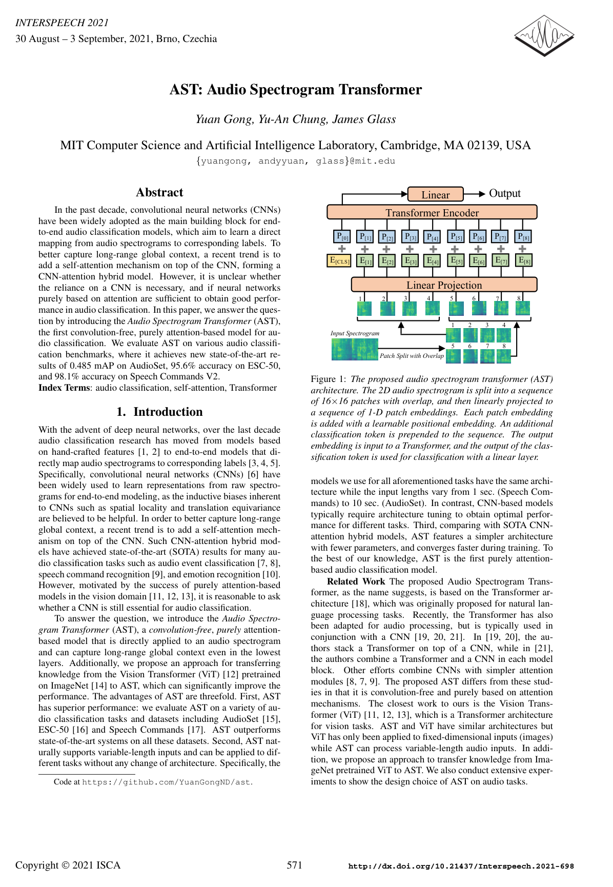
The Audio Spectrogram Transformer (AST) is a convolution-free, purely attention-based neural network for audio classification that operates directly on 2D audio spectrograms.

Given an input audio waveform of duration $t$ seconds, the front-end transforms it into a sequence of 128-dimensional log Mel filterbank features using a 25 ms Hamming window with a 10 ms hop size, yielding an audio spectrogram matrix of shape $128 \times 100t$ (128 frequency bins and $100t$ time frames).

The spectrogram is divided into a sequence of $N$ square patches of size $16 \times 16$ , extracted with an overlap of 6 bins/frames along both the frequency and time dimensions. Each $16 \times 16$ patch is flattened and linearly mapped into a 1D patch embedding vector of dimension 768 via a linear projection layer. To preserve 2D spatial context, a learnable 1D positional embedding of dimension 768 is added to each patch embedding.

A trainable classification token ([CLS]) is prepended to the sequence of patch embeddings. The combined sequence of length $N+1$ is passed through a standard Transformer encoder consisting of 12 layers, 12 attention heads, and an embedding dimension of 768. The output representation corresponding to the [CLS] token is passed through a linear projection layer with sigmoid or softmax activation to produce final classification predictions.
Knowl 2 — Patch Sequence Length Formulation for Audio Spectrograms
equation
For an audio spectrogram with 128 frequency bins and $100t$ time frames (derived from an audio waveform of duration $t$ seconds), the spectrogram is partitioned into $16 \times 16$ patches with an overlap of 6 in both the frequency and time dimensions (yielding an effective stride of $16 - 6 = 10$ ). The number of frequency patches is fixed at $\lceil (128 - 16)/10 + 1 \rceil = 12$ , and the total number of extracted patches $N$ (the effective input sequence length to the Transformer encoder) is given by:

$N = 12 \left\lceil \frac{100t - 16}{10} \right\rceil$

where $t$ is the audio duration in seconds and $\lceil \cdot \rceil$ denotes the ceiling function.
Knowl 3 — Cross-Modality Transfer Learning and Positional Embedding Adaptation
model/method
To train purely attention-based audio transformers effectively on moderate amounts of audio data, AST adapts pretrained weights from Vision Transformers (ViT) or Data-efficient Image Transformers (DeiT) trained on ImageNet:
1. Patch Embedding Layer Adaptation: ViT models take 3-channel (RGB) images, whereas AST takes single-channel spectrograms. The three sets of input channel projection weights from the ViT patch embedding layer are averaged across the channel dimension to initialize the AST single-channel linear patch projection layer.
2. Input Normalization: Audio spectrograms are normalized such that the dataset mean and standard deviation are 0.0 and 0.5, respectively.
3. Positional Embedding Adaptation (Cut and Bilinear Interpolation): A standard ViT trained on $384 \times 384$ images with non-overlapping $16 \times 16$ patches uses a positional embedding grid of shape $24 \times 24$ (576 patches). For a 10-second audio input, AST extracts a $12 \times 100$ patch grid. The $24 \times 24$ pretrained spatial positional embedding is adapted by truncating (cutting) the frequency dimension from 24 to 12 and applying bilinear interpolation along the time dimension from 24 to 100. The positional embedding of the [CLS] token is retained directly.
4. Distillation Token Handling: When adapting DeiT models that contain two class tokens (a class token and a distillation token), the two token embeddings are averaged into a single [CLS] token for audio training.
5. Classification Layer: The original vision classification head is removed, and a new linear classification layer matched to the audio label set is randomly initialized.

Knowl 4 — AudioSet Audio Event Classification Benchmark Results

data/table

AST was evaluated on the weakly labeled AudioSet benchmark (527 sound classes) across both the balanced training set (22,000 samples) and the full training set (2 million samples) using mean average precision (mAP) on the 20,000-sample evaluation set. Models were trained using binary cross-entropy loss, the Adam optimizer, mixup augmentation (ratio 0.5), SpecAugment (max time mask length 192 frames, max frequency mask length 48 bins), and epoch-wise weight averaging.

Two ensemble strategies were evaluated: Ensemble-S (averaging 3 runs initialized with different random seeds) and Ensemble-M (ensembling 6 models on the full set, or 11 models on the balanced set, spanning different random seeds, vision backbones, positional embedding adaptations, and patch split strategies).

Model	Architecture	Balanced mAP	Full mAP
Baseline	CNN + MLP	-	0.314
PANNs	CNN + Attention	0.278	0.439
PSLA (Single)	CNN + Attention	0.319	0.444
PSLA (Ensemble-S)	CNN + Attention	0.345	0.464
PSLA (Ensemble-M)	CNN + Attention	0.362	0.474
AST (Single)	Pure Attention	$0.347 \pm 0.001$	$0.459 \pm 0.000$
AST (Ensemble-S)	Pure Attention	0.363	0.475
AST (Ensemble-M)	Pure Attention	0.378	0.485

AST establishes a new state-of-the-art across all evaluated settings on AudioSet. Furthermore, AST converges in only 5 training epochs on the full AudioSet, compared to 30 epochs required by CNN-attention hybrids.

Knowl 5 — Impact of ImageNet Pretraining and Vision Backbones on AST

data/table

Ablation experiments on AudioSet demonstrate that transferring pretrained ImageNet representations is critical for attention-only audio models, especially when in-domain training data is limited.

Comparing different vision backbones initialized into AST on the balanced AudioSet indicates that higher ImageNet top-1 accuracy directly correlates with higher downstream audio classification mAP:

Pretrained Backbone	# Params	ImageNet Top-1	AudioSet Balanced mAP
ViT-Base	86M	0.846	0.320
ViT-Large*	307M	0.851	0.330
DeiT w/o Distill	86M	0.829	0.330
DeiT w/ Distill	87M	0.852	0.347

(*Note: ViT-Large was trained without patch overlap due to GPU memory constraints.)

Knowl 6 — Ablation on Positional Embedding Adaptation and Patch Overlap

data/table

Ablations on the balanced and full AudioSet training sets evaluate positional embedding adaptation techniques and patch overlap settings.

Adapting 2D positional embeddings via bilinear interpolation outperforms reinitializing positional embeddings, confirming that spatial positional knowledge transferred from vision models improves audio pattern recognition:

Increasing the patch overlap along time and frequency dimensions increases the sequence length $N$ and improves classification accuracy, at the cost of quadratic computational growth in self-attention:

Knowl 7 — Impact of Spectrogram Patch Shape and Patch Size

data/table

When trained from scratch without vision pretraining, slicing spectrograms into rectangular patches along the time axis ( $128 \times 2$ ) yields better mAP than square patches ( $16 \times 16$ ) of equal area (256 bins), as temporal ordering aligns with rectangular frames. However, because standard pretrained vision models are exclusively trained on square patches, $16 \times 16$ square patches provide superior overall performance by enabling ImageNet transfer learning. Smaller patch sizes consistently yield higher performance than larger patch sizes ( $16 \times 16$ vs. $32 \times 32$ ).

(All models in this comparison were trained on balanced AudioSet without patch overlap).

Knowl 8 — Environmental Sound Classification on ESC-50

data/table

AST was evaluated on the ESC-50 dataset (2,000 5-second environmental recordings across 50 classes) using standard 5-fold cross-validation. Models were trained for 20 epochs with batch size 48, Adam optimizer, frequency/time masking data augmentation, and an initial learning rate decayed by a factor of 0.85 per epoch after the 5th epoch (initial lr $1\times 10^{-4}$ for AST-S, $1\times 10^{-5}$ for AST-P).

AST was evaluated under two regimes: AST-S (pretrained on ImageNet only) and AST-P (pretrained on ImageNet and full AudioSet).

AST-S outperforms previous scratch-trained CNN models despite having only 1,600 training samples per cross-validation fold, and AST-P establishes a new state-of-the-art of 95.6% accuracy.

Knowl 9 — Speech Command Recognition on Speech Commands V2

data/table

AST was evaluated on the 35-class task of the Speech Commands V2 benchmark (105,829 1-second audio recordings: 84,843 train, 9,981 validation, 11,005 test). The model was trained for up to 20 epochs with a batch size of 128, Adam optimizer, an initial learning rate of $2.5 \times 10^{-4}$ decayed by 0.85 per epoch after epoch 5, and data augmentation including frequency/time masking, random noise, and mixup.

Two configurations were evaluated on the test set over 3 runs:

AST-S achieves state-of-the-art accuracy of 98.11% without any in-domain audio pretraining. AudioSet pretraining is unnecessary for this speech classification task, as AST-S outperforms AST-P.

Coverage note — No substantial contributed material was omitted. All architectural specifications, transfer learning procedures, equation formulations, benchmark datasets (AudioSet, ESC-50, Speech Commands V2), and ablation studies are fully covered.

References

1.F. Eyben, F. Weninger, F. Gross, and B. Schuller, “Recent developments in openSMILE, the Munich open-source multimedia feature extractor,” in Multimedia, 2013.
2.B. Schuller, S. Steidl, A. Batliner, A. Vinciarelli, K. Scherer, F. Ringeval, M. Chetouani, F. Weninger, F. Eyben, E. Marchi, M. Mortillaro, H. Salamin, A. Polychroniou, F. Valente, and S. K. Kim, “The Interspeech 2013 computational paralinguistics challenge: Social signals, conflict, emotion, autism,” in Interspeech, 2013.
3.N. Jaitly and G. Hinton, “Learning a better representation of speech soundwaves using restricted boltzmann machines,” in ICASSP, 2011.
4.S. Dieleman and B. Schrauwen, “End-to-end learning for music audio,” in ICASSP, 2014.
5.G. Trigeorgis, F. Ringeval, R. Brueckner, E. Marchi, M. A. Nicolaou, B. Schuller, and S. Zafeiriou, “Adieu features? end-to-end speech emotion recognition using a deep convolutional recurrent network,” in ICASSP, 2016.
6.Y. LeCun and Y. Bengio, “Convolutional networks for images, speech, and time series,” The Handbook of Brain Theory and Neural Networks, vol. 3361, no. 10, p. 1995, 1995.
7.Q. Kong, Y. Cao, T. Iqbal, Y. Wang, W. Wang, and M. D. Plumbley, “PANNs: Large-scale pretrained audio neural networks for audio pattern recognition,” IEEE/ACM TASLP, vol. 28, pp. 2880–2894, 2020.
8.Y. Gong, Y.-A. Chung, and J. Glass, “PSLA: Improving audio event classification with pretraining, sampling, labeling, and aggregation,” arXiv preprint arXiv:2102.01243, 2021.
9.O. Rybakov, N. Kononenko, N. Subrahmanya, M. Visontai, and S. Laurenzo, “Streaming keyword spotting on mobile devices,” in Interspeech, 2020.
10.P. Li, Y. Song, I. V. McLoughlin, W. Guo, and L.-R. Dai, “An attention pooling based representation learning method for speech emotion recognition,” in Interspeech, 2018.
11.A. Dosovitskiy, L. Beyer, A. Kolesnikov, D. Weissenborn, X. Zhai, T. Unterthiner, M. Dehghani, M. Minderer, G. Heigold, S. Gelly, J. Uszkoreit, and N. Houlsby, “An image is worth 16x16 words: Transformers for image recognition at scale,” in ICLR, 2021.
12.H. Touvron, M. Cord, M. Douze, F. Massa, A. Sablayrolles, and H. Jégou, “Training data-efficient image transformers & distillation through attention,” arXiv preprint arXiv:2012.12877, 2020.
13.L. Yuan, Y. Chen, T. Wang, W. Yu, Y. Shi, F. E. Tay, J. Feng, and S. Yan, “Tokens-to-token ViT: Training vision transformers from scratch on ImageNet,” arXiv preprint arXiv:2101.11986, 2021.
14.J. Deng, W. Dong, R. Socher, L.-J. Li, K. Li, and L. Fei-Fei, “ImageNet: A large-scale hierarchical image database,” in CVPR, 2009.
15.J. F. Gemmeke, D. P. Ellis, D. Freedman, A. Jansen, W. Lawrence, R. C. Moore, M. Plakal, and M. Ritter, “Audio Set: An ontology and human-labeled dataset for audio events,” in ICASSP, 2017.
16.K. J. Piczak, “ESC: Dataset for environmental sound classification,” in Multimedia, 2015.
17.P. Warden, “Speech commands: A dataset for limited-vocabulary speech recognition,” arXiv preprint arXiv:1804.03209, 2018.
18.A. Vaswani, N. Shazeer, N. Parmar, J. Uszkoreit, L. Jones, A. N. Gomez, L. Kaiser, and I. Polosukhin, “Attention is all you need,” in NIPS, 2017.
19.K. Miyazaki, T. Komatsu, T. Hayashi, S. Watanabe, T. Toda, and K. Takeda, “Convolution augmented transformer for semisupervised sound event detection,” in DCASE, 2020.
20.Q. Kong, Y. Xu, W. Wang, and M. D. Plumbley, “Sound event detection of weakly labelled data with CNN-transformer and automatic threshold optimization,” IEEE/ACM TASLP, vol. 28, pp. 2450–2460, 2020.
21.A. Gulati, J. Qin, C.-C. Chiu, N. Parmar, Y. Zhang, J. Yu, W. Han, S. Wang, Z. Zhang, Y. Wu, and R. Pang, “Conformer: Convolution-augmented transformer for speech recognition,” in Interspeech, 2020.
22.J. Devlin, M.-W. Chang, K. Lee, and K. Toutanova, “BERT: Pre-training of deep bidirectional transformers for language understanding,” in NAACL-HLT, 2019.
23.G. Gwardys and D. M. Grzywczak, “Deep image features in music information retrieval,” IJET, vol. 60, no. 4, pp. 321–326, 2014.
24.A. Guzhov, F. Raue, J. Hees, and A. Dengel, “ESResNet: Environmental sound classification based on visual domain models,” in ICPR, 2020.
25.K. Palanisamy, D. Singhania, and A. Yao, “Rethinking CNN models for audio classification,” arXiv preprint arXiv:2007.11154, 2020.
26.K. He, X. Zhang, S. Ren, and J. Sun, “Deep residual learning for image recognition,” in CVPR, 2016.
27.M. Tan and Q. V. Le, “EfficientNet: Rethinking model scaling for convolutional neural networks,” in ICML, 2019.
28.Y. Tokozume, Y. Ushiku, and T. Harada, “Learning from between-class examples for deep sound recognition,” in ICLR, 2018.
29.D. S. Park, W. Chan, Y. Zhang, C.-C. Chiu, B. Zoph, E. D. Cubuk, and Q. V. Le, “SpecAugment: A simple data augmentation method for automatic speech recognition,” in Interspeech, 2019.
30.P. Izmailov, D. Podoprikhin, T. Garipov, D. Vetrov, and A. G. Wilson, “Averaging weights leads to wider optima and better generalization,” in UAI, 2018.
31.L. Breiman, “Bagging predictors,” Machine Learning, vol. 24, no. 2, pp. 123–140, 1996.
32.D. P. Kingma and J. Ba, “Adam: A method for stochastic optimization,” in ICLR, 2015.
33.H. B. Sailor, D. M. Agrawal, and H. A. Patil, “Unsupervised filterbank learning using convolutional restricted boltzmann machine for environmental sound classification.” in Interspeech, 2017.
34.S. Majumdar and B. Ginsburg, “Matchboxnet–1d time-channel separable convolutional neural network architecture for speech commands recognition,” arXiv preprint arXiv:2004.08531, 2020.
35.J. Lin, K. Kilgour, D. Roblek, and M. Sharifi, “Training keyword spotters with limited and synthesized speech data,” in ICASSP, 2020.

Citation

MLA

Gong, Y., et al. “AST: Audio Spectrogram Transformer”. arXiv, 2021, http://arxiv.org/abs/2104.01778v3.

APA

Gong, Y., Chung, Y.-A., & Glass, J. (2021). AST: Audio Spectrogram Transformer. arXiv. http://arxiv.org/abs/2104.01778v3

Chicago

Gong, Y., Y.-A. Chung, and J. Glass. 2021. “AST: Audio Spectrogram Transformer”. arXiv. http://arxiv.org/abs/2104.01778v3.

Harvard

Gong, Y., Chung, Y.-A. and Glass, J. (2021) “AST: Audio Spectrogram Transformer”, arXiv [Preprint]. Available at: http://arxiv.org/abs/2104.01778v3.

Vancouver

1. Gong Y, Chung Y-A, Glass J (2021) AST: Audio Spectrogram Transformer. arXiv

BibTeX

@article{gong2021ast,
  title = {AST: Audio Spectrogram Transformer},
  author = {Gong, Yuan and Chung, Yu-An and Glass, James},
  year = {2021},
  journal = {arXiv},
  url = {http://arxiv.org/abs/2104.01778v3},
  eprint = {2104.01778}
}

Metadata:arXiv

Source Code

This paper has an official code repository available. Click below to access the source code.

View Repository

Access the Paper

This paper is available from its original source. Click below to access the PDF.

Open PDF

License: https://creativecommons.org/licenses/by/4.0/

Pretraining Setting	Balanced Set mAP	Full Set mAP
No Pretrain	0.148	0.366
ImageNet Pretrain	0.347	0.459

Positional Embedding Strategy	Balanced Set mAP
Reinitialize	0.305
Nearest Neighbor Interpolation	0.346
Bilinear Interpolation	0.347

Overlap Setting	# Patches ( $N$ )	Balanced Set mAP	Full Set mAP
No Overlap	512	0.336	0.451
Overlap-2	657	0.342	0.456
Overlap-4	850	0.344	0.455
Overlap-6	1212	0.347	0.459

Patch Shape Size	# Patches	w/o Pretrain mAP	w/ Pretrain mAP
$128 \times 2$ (Rectangular)	512	0.154	-
$16 \times 16$ (Square)	512	0.143	0.336
$32 \times 32$ (Square)	128	0.139	-

Model	ESC-50 Accuracy (%)
SOTA-S (Trained from scratch)	86.5
SOTA-P (AudioSet pretrained)	94.7
AST-S (ImageNet pretrained only)	$88.7 \pm 0.7$
AST-P (ImageNet + AudioSet pretrained)	95.6 $\pm$ 0.4

Model	Speech Commands V2 Accuracy (%)
SOTA-S (MatchboxNet, without extra audio)	97.4
SOTA-P (Pretrained on 200M YouTube audio)	97.7
AST-S (ImageNet pretrained only)	98.11 $\pm$ 0.05
AST-P (ImageNet + AudioSet pretrained)	$97.88 \pm 0.03$

AST: Audio Spectrogram Transformer

Abstract

Topics

Keywords

Table of Contents

Knowls

Knowl 1 — Audio Spectrogram Transformer Architecture

Knowl 2 — Patch Sequence Length Formulation for Audio Spectrograms

Knowl 3 — Cross-Modality Transfer Learning and Positional Embedding Adaptation

Knowl 4 — AudioSet Audio Event Classification Benchmark Results

Knowl 5 — Impact of ImageNet Pretraining and Vision Backbones on AST

Knowl 6 — Ablation on Positional Embedding Adaptation and Patch Overlap

Knowl 7 — Impact of Spectrogram Patch Shape and Patch Size

Knowl 8 — Environmental Sound Classification on ESC-50

Knowl 9 — Speech Command Recognition on Speech Commands V2

References

Citation

BibTeX

Source Code

Access the Paper